FAST SIMULATION OF SOLID TUMORS THERMAL ABLATION TREATMENTS WITH A 3D REACTION DIFFUSION MODEL

Abstract

An efficient computational method for near real-time simulation of thermal ablation of tumors via radio frequencies is proposed. Model simulations of the temperature field in a 3D portion of tissue containing the tumoral mass for different patterns of source heating can be used to design the ablation procedure. The availability of a very efficient computational scheme makes it possible update the predicted outcome of the procedure in real time. In the algorithms proposed here a discretization in space of the governing equations is followed by an adaptive time integration based on implicit multistep formulas. A modification of the ode15s MATLAB function which uses Krylov space iterative methods for the solution of for the linear systems arising at each integration step makes it possible to perform the simulations on standard desktop for much finer grids than using the built-in ode15s. The proposed algorithm can be applied to a wide class of nonlinear parabolic differential equations.

1. Introduction

In thermal ablation of tumors with radio frequencies (RF), it is important to be able to predict ahead of time the effects of the heating on the tumor and on the surrounding tissue. Model simulations are intended to be used before and during ablation treatments, together with temperature field images obtained by magnetic resonance to predict the effect of source placement and heating. Some recent reviews on this topic are [5] and [11].

In this paper we propose a new fast algorithm for the solution of nonlinear parabolic partial differential equations and we show that it can be used for near real-time simulation of tumor thermal ablation using the 3D model described in [10]. With the new algorithm, the time needed for running a simulation in MATLAB on a standard PC amounts to just a few seconds for high-resolution images. In general, 3D models for MR-aided thermal ablation require remarkable computational resources for the solution of large systems of nonlinear algebraic equations. In particular, if the domain is a cube discretized by subdividing each edge into n segments, several systems of O(n³) nonlinear equations with O(n³) unknowns might have to be solved during each simulation. Since in quasi Newton methods these nonlinear problems are replaced by their local affine models, their numerical solution requires, in turn, the solution of several large sparse linear systems of equations. In general, sparse direct solvers for linear systems of equations are not able to take full advantage of the multiple band structure of the Jacobian matrix of reaction diffusion models. The sparse solvers employed by the MATLAB function ode15s adhere to this paradigm. Therefore the coefficient matrices of the resulting linear systems are treated as a 2n²-banded matrices, thus requiring, as n increases, large amount of memory allocation, O(n⁵) cells, and computational time, O(n⁷) floating point operations.

The computational efficiency of the algorithm that we propose here comes from the use of Krylov subspace iterative methods for the solution of the large and sparse linear systems arising during the simulations. This reduces the amount of memory to O(n³) cells and the computational time to O(n⁴) floating point operations. Krylov subspace methods are used here as iterative solvers, i.e., given an initial approximate solution x₀, these algorithms compute a sequence of approximations. Krylov subspace iterative linear solvers at each iteration seek a new approximate solution in the affine subspace x₀ + K_m, where x₀ is an initial guess and K_m is the Krylov subspace of ℝⁿ of dimension m ≤ n:

$$K_m=\text{span}\{v,Av,A^{2}v,\dots A^{m-1}v\},$$

Here A is the coefficient matrix of the system linear system that we want to solve and v is a vector related to the initial residual vector. The (unique) approximation x_m at step m is determined by using an orthonormal basis for K_m determined during the iteration steps. More specifically, the next residual vector is constrained to be orthogonal to m linearly independent vectors defining a subspace L_m of dimension m which is called the subspace of constraints. The choice of subspaces varies for different Krylov subspace linear system solvers. This framework is known as the Petrov-Galerkin conditions; see [13, Chapter 6] for details. A description of the Krylov subspace linear solver that we will consider here, i.e., Conjugate Gradient, can be found in Phase 3, section 3.3.

2. Thermal ablation models

Following Johnson and Saidel in [10], we consider a model where the tumor is located at the center of a cube of tissue large enough that the temperature at the boundary of the region is not affected by the heating. We assume that a radio frequency delivered through a probe inserted into the tumor induces ohmic current that acts like a heat source. The heat is, in turn, dissipated by thermal conduction through the tissue and uptaken by the blood flowing through the vessels perfusing the tissue; see [10] for details.

The time course of the temperature profile in the tumor and in the surrounding tissue during the ablation procedure is described by the time-dependent partial differential equation

$$\frac{\partial T}{\partial t}=\alpha \Delta T-\omega (r,t,T){[T-T_b]}_{+}+\sigma (r,t),t>0,(x,y,z)\in \Omega .$$ (2.1)

Here T = T(x, y, z, t) is a function of the position vector r = (x, y, z) and of time, and the domain Ω is the 3D cube [−L,L] × [−L,L] × [−L,L]. We also assume that the temperature on the boundary of the cube remains constant and equal to the basal temperature, i.e.,

$$T=T_b,(x,y,z)\in \partial \Omega ,$$

since the heat source is sufficiently far from the boundaries of the cube.

The value of the parameter α is considered constant here, α = α₀; however, our approach can be easily generalized to the case where α is a function of T. The perfusion factor ω(r, t, T) depends on the thermal tissue response to the ablation and is inversely proportional to the coagulation factor. In general, ω is described in terms of a probabilistic model reflecting the local variability of the thermal response,

$$\omega (r,t,T)={\omega }_0\exp \left({\int }_0^t\beta (r,t)\mathit{dt}\right),$$ (2.2)

where the transition probability can be represented by an Arrhenius model of the form

$$\beta (r,t,T)=\delta (T-T_0)\cdot A\exp (-B∕T(r,t)),$$

where δ(·) is the unit step function. A list of the values of the parameters specifying the model can be found in Appendix II. For more parameters, see [10]. Alternatively we can consider a simplified model, where perfusion exists locally in the tissue as long as the tissue temperature is below a critical value T_c:

$$\omega (r,t,T)={\omega }_0\cdot \delta \left({[T_C-T]}_{+}\right).$$ (2.3)

In our simulations we considered both perfusion models for ω and found negligible differences in term of computational cost in the performances of our algorithm.

The probe is modelled as a uniform line segment located along the Z axis from −L_p to L_p. Each point on the probe is identified by the 3D position vector r_p. Therefore, since the RF heat source σ(r, t) varies inversely with the square of the distance from the probe, we can write the source term σ in the form

$$\sigma (r,t)=h_p\left(t\right)∕{(r-r_p)}^2,r\ne r_p.$$ (2.4)

For our numerical simulations, h_p(t), the measured input power, will be taken constant. The probe temperature is given by

$$T_p\left(t\right)=T_b+T_{\Delta }(1-\exp (-t∕\tau )),$$ (2.5)

where τ is response in time. The value of the constant T_Δ is determined by imposing that T_p(∞) = T_Δ + T_b is the maximum possible value for the temperature of the probe.

3. The proposed algorithms

In order for the simulations to be of help during the magnetic resonance guided treatment, we should be able to compute the solution of (2.1)-(2.5) very fast on a personal computer, possibly with a spatial resolution of the order of the resolution of the MR images collected during the procedure. The algorithm that we propose here has all the features needed for interactive, real-time applications.

We present the description of the algorithm in three parts. First we address the issue of the space discretization of (2.1) which transforms the original partial differential equation into a system of ordinary differential equations. In step 2 we discuss the issues which have to be taken into account when choosing a suitable time integrator for this system of ordinary differential equations. Step 3 is devoted to the efficient solution, at each time step, of large systems of nonlinear and linear algebraic systems.

3.1. Phase 1: Semidiscretization in space

The right hand side of the partial differential equation (2.1) is the sum of three terms. The first one is the diffusion term, which can be either linear or nonlinear depending on the choice of α; here it is linear since α is constant; the second one is the (nonlinear) reaction term and the third one is the source term from RF energy.

We consider here approximations of the spatial partial derivatives in the diffusion term in each direction by means of centered differences of order two and four, respectively. These approximations are obtained with the stencils detailed below.

Let the functions w_i,j,k(t), i, j, k = 1, …, n approximate the continuous solution T(t, x, y, z) at the time instant t for x = x_i, y = y_j, z = z_k,

$$x_i=-L+i\cdot h,y_j=-L+j\cdot h,z_k=-L+k\cdot h,i,j,k=1,\dots ,n,$$

where h = 2L/(n + 1) is the constant stepsize used in each space direction. The second order centered differencing approximation for the 3D operator αΔw in (2.1), with the dependence from the temporal variable t omitted to simplify the notation, is given by

$$\frac{\alpha }{h^2}(w_{i-1,j,k}+w_{i,j-1,k}+w_{i,j,k-1}-6w_{i,j,k}+w_{i+1,j,k}+w_{i,j+1,k}+w_{i,j,k+1}),$$ (3.1)

i, j, k = 1, …, n. Whenever one or more of the indices i, j, k are equal to 0 or to n + 1, the functions w_i,j,k(t) in (3.1) are determined by the underlying initial-boundary value problem.

The fourth order centered approximation for αΔw in (2.1) is given by

$$\begin{array}{cc}\hfill & \frac{\alpha }{h^2}(-\frac{1}{12}{w}_{i-2,j,k}-\frac{1}{12}{w}_{i,j-2,k}-\frac{1}{12}{w}_{i,j,k-2}+\frac{4}{3}{w}_{i-1,j,k}+\frac{4}{3}{w}_{i,j-1,k}\hfill \\ \hfill & +\frac{4}{3}{w}_{i,j,k-1}-\frac{15}{2}{w}_{i,j,k}+\frac{4}{3}{w}_{i+1,j,k}+\frac{4}{3}{w}_{i,j+1,k}+\frac{4}{3}{w}_{i,j,k+1}\hfill \\ \hfill & -\frac{1}{12}{w}_{i+2,j,k}-\frac{1}{12}{w}_{i,j+2,k}-\frac{1}{12}{w}_{i,j,k+2}),i,j,k=1,\dots ,n.\hfill \end{array}$$ (3.2)

When one or more of the indices i, j, k are equal 0 or n + 1, the values of the functions w_i,j,k(t) in (3.2) are “borrowed ”, as for the second order formulas, while when one or more of the indices i, j, k equal −1 or n + 2, fictitious values need to be introduced. In the models that we consider, they are determined by the underlying initial-boundary value problem. In particular, since our domain is a cube of tissue surrounding the tumor large enough that the thermal ablation effects are not reaching the boundaries of the domain, these values are assumed to remain constant and equal to the basal temperature T_b.

We remark that since the nonlinear reaction term and the source term do not contain any spatial derivatives, they do not need be considered in this phase; see, e.g., the discussions in [9].

Therefore, after discretizing in space (2.1), we get a family of system of n³ nonlinear differential equations parametrized by the spatial stepsize h:

$$\frac{d}{\mathit{dt}}T\left(t\right)=\alpha \mathit{LT}\left(t\right)-{\omega }_{0}D\left(T\right)+\sigma \left(t\right),t>0,$$ (3.3)

where the source term

$$\sigma \left(t\right)=T_p\left(t\right)\cdot v_{\mathit{probe}}\left(t\right)+T_b\cdot v_{\mathit{bc}}$$

now takes into account the contribution of the probe, whose temperature at time t is T_p(t), and of the Dirichlet boundary conditions. The initial profile T(0) is the n³ vector whose entries are all equal to the basal temperature T_p.

We note that only the first two terms, diffusion and reaction, depends on the unknown function T(t, x, y, z). The nonlinear diagonal matrix function D(T) in the reaction term is obtained by evaluating (2.3) (or (2.2)) at T. When the diffusion coefficient α = α₀ is constant, as in our setting, L is a n³ × n³ symmetric matrix with real entries determined by the stencil (3.1) or (3.2). Whether we use second or fourth order approximation, the matrix L is very sparse, with only O(N) nonzero elements, where N is the number of interior points in the spatial grid, and banded, with the most external bands O(n²) elements away from the main diagonal. The distance of the outmost band from the main diagonal poses a big challenge when using a direct solver, as we will discuss in Step 3.

The properties of the Jacobian matrix of (3.3) play a crucial role in the selection of a suitable time integrator and of an iterative method for the solution of the associate systems of algebraic equations.

Let us denote by J the Jacobian matrix of (3.3). If we assume the threshold model (2.3) for perfusion, the Jacobian is of the form

$$J=\{\begin{array}{cc}\alpha L-{\omega }_0\delta \left({[T_c-T]}_{+}\right)I,\hfill & T_c\ge T,\hfill \\ \alpha L,\hfill & T_c<T,\hfill \end{array}\phantom{\}}$$ (3.4)

where I is the identity matrix.

Since L is symmetric and negative definite, α, ω₀ are positive and δ(·) can assume only the values 0 or 1, then J is also negative definite. In particular, it can be shown (by using results on generating function; see, e.g., [12, Section II.3.5]) that the eigenvalues of J satisfy

$$-\frac{\alpha }{h^2}12\le {\lambda }_j\left(L\right)<0,$$

when using second order spatial finite differences, and

$$-\frac{\alpha }{h^2}\frac{47}{4}\le {\lambda }_j\left(L\right)\le -\frac{\alpha }{h^2}\frac{15}{4}$$

for fourth order. Note that the minimum eigenvalue of L for the fourth order discretization is slightly greater than for the second order.

The Jacobian matrices related to the two spatial discretizations are both n³ × n³ and banded but they do differ for the number of nonzero bands. In particular, when using the second order formula, the nonzero elements of the Jacobian matrix are located along 7 nonzero diagonals while when using the fourth order the number of nonzero diagonals increases to 13; see Figures 3.1 and 3.2, respectively. Therefore, the number of floating point operations for computing a single matrix-vector product is slightly less than doubled with the higher order discretization; see Performance comparisons section. However, changing the order of the spatial discretization requires a new choice of the tolerances for the iterative solvers for the inner and outer iterations, to maintain a balance between the time and space components in the error term. We will turn to this point at the end of Phase 3.

Fig. 3.1.

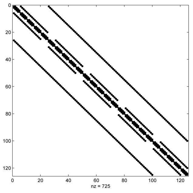
Pattern of the nonzero entries for the Jacobian matrix related to the second order discretization with n = 5. The tight band around the main diagonal has width 3.

Fig. 3.2.

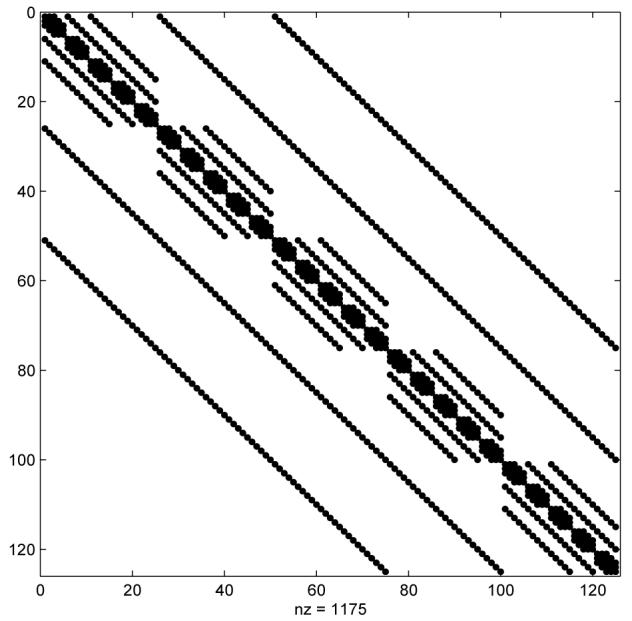
Pattern of the nonzero entries for the Jacobian matrix related to the fourth order discretization with n = 5. The tight band around the main diagonal has width 5.

3.2. Phase 2: Advancing in time

The model (2.1) under consideration has a dominant parabolic character, since the coefficient of the diffusion term αΔT, α = 0.15, is about 20 times larger than the coefficient of the reaction term, where ω₀ = 0.007; see [10]. Therefore the system of differential equations (3.3) is stiff. It is well known that explicit integrators for ordinary differential equations (ODE for short) are not suitable for the solution of stiff systems because, in order to guarantee the numerical stability of the method, it is necessary to make sure that the Courant-Friedrichs-Lewy condition (CFL for short) is satisfied; see, e.g., [15]. Here this means that the limited size of the stability region of all explicit, and some of the implicit methods forces the integrator to use time steps proportional to the square of the discretization step in space; see, e.g., [15]. The constraint on the length of the time step is particularly burdensome in the case where the time interval of the simulation is long, as in the problem that we consider here. Computed examples with explicit time integrators, e.g., explicit Runge-Kutta methods or explicit multistep formulas, showed an increase of the overall computation time of orders of magnitude even for moderate spatial resolutions. Thus, since the length of time of the simulations of the ablation treatments exceeds 10 minutes, the use of explicit time integrators is not feasible. For example, with the parameter values in Appendix II, the total amount of work with the explicit MATLAB time integrator ode45 is of the order of 10⁷ times more than with the implicit integrator ode15s with the same tolerances required for the local error estimation. We recall that ode45 is a MATLAB package based on the embedded Runge-Kutta-Fehlberg formulas of orders 4 and 5. For more information about these and other time-step integrators in MATLAB, see [14].

A k-step (1 ≤ k ≤ 5) implicit linear multistep method like the built-in Matlab function ode15s is based on the formula

$$\sum _{j=0}^k{\alpha }_j{T}_{n+j}=\tau \sum _{j=0}^k{b}_j{f}_{n+j},n=0,1,\dots ,$$

where f(t,T) is the right hand side of (3.3), τ = τ(n) is the time step and f_n+j = f(t_n+j,T_n+j), T_n+j ≃ T(t_n+j) approximates the temperature at time t_n+j.

Since ode15s is a variable-step, variable-order, from order 1 to order 5, solver based on Backward Differentiation Formulas (BDF) which are all at least A₀-stable, it can handle stiff ODE systems whose Jacobian matrices have negative real eigenvalues without any stepsize restrictions due to stability requirements. If the step size used is very large, the accuracy of the computed solution may be low, but it will not be contaminated by unstable spurious components. This can be very helpful in finding crude estimates of the solution at a small computational cost.

The big computational bottleneck of implicit time integrators is the need to solve, at each time step, a system of algebraic equations of the dimension of the number of the spatial nodes. In our problem, at each time step we need to solve a system of nonlinear equations, which can be quite a challenging task due to the three dimensionality of the problem. Our goal in this paper is to present a modification of ode15s which used Krylov subspace iterative methods for the solution of the systems of linear equations, thus taking full advantage of the sparsity pattern of the Jacobian matrices.

Another package for time integrator suitable for the solution of stiff systems of ordinary differential equations based on implicit Runge-Kutta formulas is Radau5; see [8] for more details. Although Krylov subspace methods could be used also for the solution of linear systems in Radau5, the results of preliminary computed examples strongly suggest that, even with the use of Krylov iterative linear systems solvers the method is not competitive with ode15s for the present problem. The much longer computing time needed for the simulations when using radau5 is due to the fact that the linear systems arising in Radau5 are three times larger, i.e., 3n³ × 3n³ × vs n³ × n³ and with triple bandwidth than those arising in ode15s. More precisely, the coefficient matrix in the quasi Newton step of the Radau5 is of the form

$$M_n=(I-\tau \mathit{bA}\otimes J_n),$$ (3.5)

where ⊗ is the Kronecker product, A is the s × s matrix of the s-stages implicit Runge-Kutta method (s = 3 for Radau5) and J_n is the scaled Jacobian, computed only once at each time step. Although the matrix M_n can be block-diagonalized following the diagonalization of A, and the linear system decouples into s linear systems of size n³, we still need to multiply the computational cost approximately by s, the number of the stages of the method. Without decoupling, the computational cost for the solution of each linear system (3.5) can increases asymptotically by a factor of up to nine.

In summary, we found ode15s to be most efficient for the solution of our parabolic problem with Dirichlet boundary conditions whose Jacobian matrix is symmetric with real non positive eigenvalues. In fact, for the unconditional stability of (2.1)-(3.3), it suffices that the negative real axis is included in the absolute stability region for the considered time-marching scheme. Methods which have this stability property are called as A₀-stable; see, e.g., [8]. Time integrators with a wider absolute stability region, like Radau5, which are usually more expensive, are better suited for problems whose Jacobian matrices do not necessarily have purely real eigenvalues.

3.3. Phase 3: Solution of the discrete problem

The application of ode15s to the system of differential equations arising from the finite difference discretization in space of (2.1) with stepsize h requires the solution of systems of n³ algebraic linear and nonlinear equations for T_n+k. We begin with recalling how to compute an approximation of the value of T(t_n+k) by a quasi Newton algorithm with the Jacobian matrix computed once at the beginning of the iteration. More precisely, at the rth quasi Newton iteration, we first compute the solution s^(r) of

$$\left(a_{k}I-\tau b_k{\phantom{\mid }\frac{\partial f(t,T)}{\partial T_{n+k}}\mid }_{T_{n+k}^{\left(0\right)}}\right)s^{\left(r\right)}=-F\left(T_{n+k}^{\left(r\right)}\right),$$ (3.6)

then we update

$$T_{n+k}^{(r+1)}=T_{n+k}^{\left(r\right)}+s^{\left(r\right)},r=0,1,\dots .$$

We continue iterating until $\Vert T_{n+k}^{(r+1)}-T_{n+k}^{\left(r\right)}\Vert$ and $\Vert F\left(T_{n+k}^{(r+1)}\right)\Vert$ are sufficiently small. Note that

$$F\left(T_{n+k}^{\left(r\right)}\right)=a_k{T}_{n+k}^{\left(r\right)}-\tau b_k{f}_{n+k}^{\left(r\right)}+g(T_n,\dots ,T_{n+k-1}),$$

where g is a function of f and of the approximations of T at the points t_n, t_n+1, …, t_n+k−1. The time step τ in ode15s changes adaptively.

It is clear that, since the main computational task in implicit time integrators is the repeated solution of systems of linear equation, by designing a more efficient linear system solver which is still compatible with the accuracy requirement of the integrator, we will be able to significantly reduce the overall computing time.

Sparse direct linear system solvers usually require factorization of the coefficient matrix in (3.6) whenever, e.g., the value of τ changes. For an n × n × n mesh, the cost of a direct sparse factorization is proportional to n³ times the square of the bandwidth of the Jacobian matrix of (3.3). We remark that matrices with a small number of nonzero diagonals, for example 7 or 13 as in the proposed second and fourth order discretizations in space, respectively, generate factorizations with a large bandwidth, in our case proportional to n², due to the location of nonzero diagonals. This phenomenon is typical of multidimensional finite differences (finite volumes, finite elements) discretizations. Thus the number of floating point operations needed for each direct sparse factorization is proportional to n³ ·(O(n²))² = O(n⁷). In addition, the O(n⁵) floating-point memory cells needed to store the intermediate steps of the factorization, make the method unfeasible for usage on standard personal computers even for relatively rough meshes.

The large dimensionality of the linear systems arising from the three dimensionality of the problem, and the sparsity of the Jacobian make this an ideal setting for using Krylov subspace iterative solvers. Krylov subspace iterative methods are routinely used for the solution of large, sparse linear system of equations. Among them, the most popular ones are the Conjugate Gradient (CG) method, applicable when the coefficent matrix is symmetric positive definite, the biConjugate Gradient (biCG), and the Generalized Minimal RESidual (GMRES) methods, which are applicable to more general linear systems; see [13] for details. A basic version of Conjugate Gradient algorithm is sketched below.

$$\begin{array}{cc}\hfill & \mathit{Basic}\mathit{Conjugate}\mathit{gradients}\mathit{for}\mathit{solving}Ax=b\hfill \\ \hfill & x_0\text{assigned},r_0=b-{\mathit{Ax}}_0;p_0=r_0\hfill \\ \hfill & \text{For}k=1,2,\dots \hfill \\ \hfill & {\alpha }_{k-1}=(r_{k-1},{\mathit{Ap}}_{k-1})∕({\mathit{Ap}}_{k-1},{\mathit{Ap}}_{k-1})\hfill \\ \hfill & x_k=x_{k-1}+{\alpha }_{k-1}{p}_{k-1}\hfill \\ \hfill & r_k=r_{k-1}-{\alpha }_{k-1}{\mathit{Ap}}_{k-1}\hfill \\ \hfill & {\beta }_{k-1}=({\mathit{Ar}}_k,{\mathit{Ap}}_{k-1})∕({\mathit{Ap}}_{k-1},{\mathit{Ap}}_{k-1})\hfill \\ \hfill & p_k=r_k-{\beta }_{k-1}{p}_{k-1}\hfill \end{array}$$

Conjugate Gradient method, at each iteration, minimizes the energy norm of the difference between the computed approximation and the true solution; see [13, section 6.11].

Krylov subspace iterative linear system solvers, given an initial approximate solution, compute a sequence of approximate solutions requiring the coefficient matrix only as a multiplier for an arbitrary vector. Furthermore, when using iterative methods it is possible to solve the linear systems (3.6) only up to a desired accuracy. This last feature is particularly convenient when solving nonlinear differential equations, since in the first few quasi Newton iterations it suffices to solve the linearized problem only approximately. This strategy is sometimes referred to as inexact Newton in the literature; see [6] for details.

Since, when solving nonlinear systems by inexact Newton method we have two nested iterative algorithms, the outer quasi Newton step and the the inner iterative linear system solver, we will refer to them as inner and outer iterations in the remainder of the paper. In our problem, for a n × n × n mesh, at each outer iteration step we need to solve an n³ × n³ system of linear equations whose coefficient matrix M_n+k symmetric positive definite; see the right hand side of (3.3). Furthermore, the matrix M_n+k is banded with the same nonzero diagonals of the matrix L, which is in turn related to the discretization in space of α(T)ΔT in (2.1). Here we assume that α is constant; the extension to α = α(T), with α(T) a diagonal matrix, is straightforward. The iterative solution of linear systems of this form is very efficient even for large values of n. In fact, Krylov iterative solvers require only c₁d·n³ floating point operations per iteration (one or two matrix by a real-valued vector products per iterations; see, e.g., [13]), where c₁ is a constant of the order of unity and d is the number of nonzero diagonals of the Jacobian matrix. Moreover, these iterative solvers when applied to (3.6) converge in at most c · n iterations, where c is a small constant, without preprocessing (3.6); see Appendix I. The number of inner iterations may be reduced by preprocessing the underlying linear systems with suitable preconditioners when τ in (3.6) is large (otherwise preconditioning is not needed at all.) However, there are a couple of considerations which suggest us to avoid preconditioning here. First, since convergence takes place after a moderate number of iterations, it seems that for our problem preconditioning can be beneficial only with a careful implementation and for very large values of n. Second, preconditioning gives an approximate solution which is no longer more accurate in the dominant subspace, i.e. along the eigenvectors of the matrix in (3.6) related to eigenvalues connected with stiffness phenomenon, but in the dominant subspace of the matrix of the underlying transformed problem; see [7]. Therefore, we will not pursue the issue any further here. Preconditioning strategies for parabolic time dependent problems has been proposed in [1, 3].

The overall asymptotic computational cost ranges from c₂ × n³ to c₃ × n⁴, where c₂ and c₃ are constants of the order of unity. This cost is much less than when using direct solver for linear systems (3.6). Moreover, unlike for direct solvers, for Krylov iterative solvers there is no need for extra memory space for intermediate matrices.

Tolerances and stopping criteria for iterative algorithms

Implicit time integrators, including ode15s and radau5, routinely allow only very few steps of outer iteration prior to reducing the step size τ.

We observe that, when using a time integrator based on implicit formulas which utilizes an iterative linear system solver, in the first few outer iterations, when the error in the outer step is still large, it suffices to carry out only as many inner iterations as needed to solve the linear system within a tolerance related to an estimate of the error in the outer step. Therefore in our computed examples at the rth outer step we stop the inner iterations as soon as the relative residual is less or equal to

$$\max \{\mathit{tol},{10}^{-2\cdot r}\},$$

where tol is a prescribed minimum admitted tolerance for the inner iterative solver. The introduction of this simple stopping criterion for the inner iterations causes a sensible decrease in the total number of inner iterations, yielding a solution analogous to that obtained when using sparse direct solvers. Further reduction of the overall computational time may be achieved by a fine tuning of the parameters which control the termination of inner and outer iterations.

The theoretical results regarding inexact Newton iterations indicate that the tolerances for terminating the inner and outer iterations should be gradually increased up to a constant times the tolerance for the local relative error of the time-step integrator. For computational efficiency, the discretization parameters should be chosen carefully to avoid that errors generated by the discretization in time dominate over those in space or vice versa. Indeed, the global error can be bounded by [9]

$$\Vert T_h\left(t_n\right)-{\tilde{T}}_n\Vert \le \Vert T_h\left(t_n\right)-\tilde{T}\left(t_n\right)\Vert +\Vert \tilde{T}\left(t_n\right)-{\tilde{T}}_n\Vert \le \tilde{c}{h}^p+\widehat{c}{\tau }^q,$$

where T_h(t_n) is the exact solution of the projection of (2.1) onto the mesh nodes, T̃(t) is the exact solution of the ODE (3.3) arising after the discretization in space, T̃_n is the computed approximate solution obtained by first discretizing in space and then integrating (3.3) in time, and h, p and τ, q are the step size and order of the discretizations in space and time, respectively.

4. Performance comparisons for thermal ablation simulation

We compare the performance of the proposed iterative version of ode15s to that of the MATLAB v.7.0 built-in ode15s for the simulation of thermal ablation of tumors via radio frequencies over an interval of time of 600 seconds. We start with a rather coarse 3-dimensional grid, n = 11, and we test the algorithm for finer and finer grids, up to n = 61. The linear systems in the iterative version of ode15s were solved by CG method. We also verifies that comparable results are obtained when using biCGStab, a variant of the biCG algorithm known for its improved numerical stability for problems with a nonsymmetric Jacobian.

All experiments were performed on a laptop Pentium IV 3Ghz with 2Gb Ram. Parameters for the simulation were set equal for the two algorithms and reported in Appendix II. In Table 1 we report the performance results for our simulations when using a second order discretization in space, while the analogous results for the forth order discretization are presented in Table 2. In the first two columns of the table we indicate the number of nodes in each space dimension and the total number of mesh nodes. The third column, labeled resolution, reports the spatial resolution of the simulation in millimeters. The three columns grouped under the iterative heading summarize the performance of our iterative version of ode15s. More specifically, in the column labeled time, we report the total time required by the simulation, in the avg and total it column we lists the average number of inner iterations needed for the solution of a linear system of equations, and the total number of inner iterations. Note that each CG iteration requires one matrix-vector product.

Table 4.1.

Performance comparison for the threshold model. The second order approximation is used for discretization in space.

Grid			Iterative			Direct
n	size	resolution	time	avg	total it	time	lu dec
11	1331	3.90 mm	2.34s	9.7	1762	6.0s	28
21	9261	2.13 mm	27.4s	15.7	3808	7'55s	35
31	29791	1.46 mm	2'18s	20.7	5647	n/a	n/a
41	68921	1.11 mm	11'12s	26.7	8295	n/a	n/a
51	132651	0.90 mm	31'49s	30.6	10387	n/a	n/a
61	226981	0.75 mm	78'24s	36.0	12803	n/a	n/a
71	357911	0.65 mm	2h 52'	40.6	15448	n/a	n/a

Table 4.2.

Performance comparison for the threshold model. Parameter as in Table 4.1 with fourth order approximation for discretization in space.

Grid			Iterative			Direct
n	size	resolution	time	avg	total it	time	lu dec
11	1331	3.90 mm	8.9s	11.9	5792	44.8s	74
21	9261	2.13 mm	1'25s	20.0	11197	1h	85
31	29791	1.46 mm	6'23s	25.3	13936	n/a	n/a
41	68921	1.11 mm	25'12s	31.7	18179	n/a	n/a
51	132651	0.90 mm	61'25s	37.0	21320	n/a	n/a
61	226981	0.75 mm	2h 16'	42.3	24898	n/a	n/a

The results pertinent to the performance of the built-in ode15s are displayed in the two columns grouped under the “Direct” heading. In addition to the time required for the simulation, we report the total number of factorizations required for the simulation (column labeled LU). An n/a entry means that the computer was unable to complete the simulation run because of insufficient memory. It is quite remarkable that, while with the iterative version ode15s we can used grids of size up to n = 71, with the built-in ode15s we cannot even use a grid corresponding to n = 31 because of the number of memory cells, ranging from O(n⁵) to O(n⁶), needed for the matrix factorizations.

The results from our simulations show that with the iterative version of ode15s, the numbers of iterations needed to solve each linear system seems to increases at most linearly with n, in agreement with the result proved in Appendix I. The total time of the simulation also grows at most linearly with the size n³ of the Jacobian. The tables show that with the iterative version ode15s the total number of inner iterations and the overall computation times increase slightly as we go from second to fourth order discretization in space. This is not the case for the built-in ode15s, where we have a three fold increase in the computational time when we pass from second to fourth-order discretization in space.

In Figure 4.1 we show the temperature distribution along the XZ plane after 600 seconds by using the second order approximation for the Laplace operator.

Fig. 4.1.

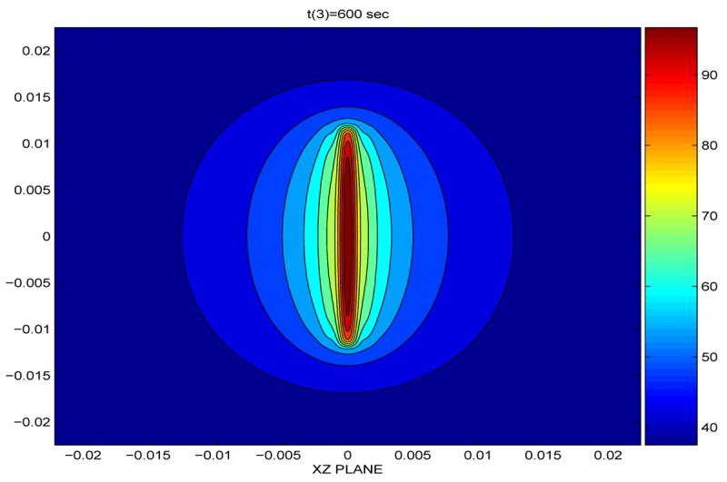
Temperature distribution (in Celsius degrees) along the XZ plane after 600 seconds; n=61, resolution:0.75 mm (the unit in the plot is 1 meters=10³ mm). Parameter as in Table 4.1

Repeated simulations of thermal ablation using a MATLAB version of the Radau5 method with sparse direct linear system solvers confirmed the superiority, from the point of view of computational efficiency, of the iterative version of ode15s. This is not surprising since, as pointed out in previous Section, the systems of algebraic equations which need to be solved inside Radau5 are three times larger than those arising in ode15s, and the bandwidth of the Jacobian matrix increases by the same factor. For example, with n = 11 and second (fourth) order discretization in space, Radau5 requires 94 (114) seconds, while only 2.3 (9) seconds are needed by ode15s with the order of the method fixed to 5. Because of these performances, we think that we can speak of “near real time” simulations. Of course, by a careful implementation of the proposed strategies in a compiled language, the timings we show can be even more dramatically reduced.

5. Conclusions

The use of iterative methods for solving the linear systems arising in the solution of time-dependent partial differential equations has been shown to be very beneficial for certain classes of problems; see [2]. However, since for a reliable and efficient use of iterative solvers it is necessary to analyze and understand the properties of the systems to be solved, traditionally direct methods have been preferred.

The use of iterative methods in the context of solving time dependent partial differential equations in three dimensions becomes mandatory for medium to fine grids. In this paper we show that by replacing the sparse direct solvers in the MATLAB function ode15s by Krylov subspace iterative methods, it is possible to run simulations of thermal ablation of tumors in three dimensional grids with good spatial resolution even on personal computers.

Biographies

Daniele Bertaccini has received his Ph.D (“Dottorato”) in Mathematics in 1999 from Universita' di Firenze, Italy. He is currently a professor in the Dipartimento di Matematica at Universita' di Roma “La Sapienza“, Roma, Italy. His research interests include fast algorithms for large and sparse discrete models, numerical time integration for partial differential equations and applications to life sciences.

Daniela Calvetti has received her M.S. and Ph.D. in Mathematics in 1985 and 1989, respectively, from the University of North Carolina at Chapel Hill. She is currently a professor in the Department of Mathematics and a member of the Center for Modelling Integrated Metabolic Systems at Case Western Reserve University.

Appendix I. Convergence of inner iterations

We now prove the claim that the number of inner iterations without any preconditioning is bounded above by n, the number of subdivision of the grid for each side. Let us denote by κ(M) the 2-norm condition number of a symmetric definite, positive or negative, matrix M. We have that

$$k\left(M\right)=\frac{\Vert M{\Vert }_2}{\Vert M^{-1}{\Vert }_2}=\frac{{\max }_j{\lambda }_j\left(M\right)}{{\min }_j{\lambda }_j\left(M\right)}.$$

Let A be a symmetric positive definite matrix. The A-norm of a vector v is defined as

$$\Vert v{\Vert }_A=v^T\mathit{Av}.$$

The mth iterate of the Conjugate Gradient algorithm minimizes the A-norm of the error e_m = x_m − x_*, where x_* is the exact solution of the linear system. From this property, it can be shown that

$$\Vert e_m{\Vert }_A\le 2{\left(\frac{\sqrt{k\left(M\right)}-1}{\sqrt{k\left(M\right)}+1}\right)}^m\Vert e_0{\Vert }_A,$$ (5.1)

see, e.g., [13, Chapter 6]. However, if we consider the linear system (3.6), we get

$$1<k\left(M_{n,k}\right)\le \tau k\left(J\right)\le O\left(\frac{\tau }{h^2}\right)=O\left(\tau n^2\right),$$

for both the second and fourth order approximations in space. Therefore, at the mth iteration we decrease the relative error by p orders of magnitude, p≥1, provided that

$$2{\left(\frac{\mathit{cn}-1}{\mathit{cn}+1}\right)}^m<{10}^{-p}.$$

Taking the logarithm of both sides and using Taylor series expansion for

$$\log \left(1+\frac{2}{\mathit{cn}-1}\right),$$

shows that m is proportional to p · n.

Appendix II. Parameters of the model

The parameters used in simulations are detailed below.

• t ∈ [0, 600] s (simulation time in seconds)

• L_p = (46.8/4) mm (1/2 length of the probe)

• L = (46.8/2) mm (1/2 side of the cube)

• α₀ = .15 mm²/^s

• ω₀ = 0.007

• T_b = 37°C (basal temperature)

• T_pm = 90°C (maximum temperature for the probe)

• T_c = 60°C (threshold for model with perfusion)

• T₀ = 41°C

• h_p = 4.0 (input power for the probe)

• τ = 20s

• Parameters for Arrhenius-type perfusion:

• A= 2.9e · 10³⁷ B= 3 · 10⁴.

Appendix III. Assembling the Jacobian matrix in MATLAB

The simulation can be implemented in a simple, meaningful and computationally efficient way provided that the construction is performed in a vector-oriented fashion, which takes full advantage of the MATLAB features. The user interface of ode15s routine is described in detail in [14, Section 6]. For the convenience of interested readers, we outline in this appendix how to assemble the Jacobian in a MATLAB oriented fashion. The first step is the construction of the discretized Laplace operator L, for which the following commands can be used (for the second order discretization):

e=ones(n,1); I=speye(n);

L1=(alpha/(h^2))*spdiags([e −2*e e],−1:1,n,n);

L=kron(L1,kron(I,I)+kron(I,kron(L1,I))+kron(I,kron(I,L1)));

The initial and boundary conditions are placed in the same source file in the three vectors T₀ vbc and vbc2, where we encode the appropriate information about the probe and the temperature on the domain Ω. In the next step we need to write a MATLAB function which defines the system of differential equations (3.3). For this purpose, after placing the discrete Laplacian matrix L and the vectors with the boundary conditions in a global variable, we write the derivative dT of the function T as the sum of four terms:

% first part: the discrete diffusion operator

dT=L*T;

% second (constant perfusion + threshold)

vec=((Tc*e-T)>0);

D=spdiags([vec],0,n3,n3);

dT=dT−omega0*D*(T-e*Tb);

% third (source)

dT=dT+sigma;

% fourth: boundary conditions

Tp=Tb+Tdelta*(1−exp(−t/tau)); % temperature of the probe

dT=dT+Tp*vbc; % the probe's thermal influence

dT=dT+Tb*vbc2; % boundary conditions on the cube's faces

We remark that before calling the implicit time integrator, the options vector needs to be set so that the sparsity pattern of the Jacobian matrix and the preferred linear multistep formulas, BDF in the case of ode15s, are specified.

The MATLAB code for the iterative version of ode15s can be obtained by contacting the first author.

REFERENCES

- 1.Benzi M, Bertaccini D. Approximate inverse preconditioning for shifted linear systems. BIT. 2003;43:231–244. [Google Scholar]
- 2.Bertaccini D, Ng Michael K. Band-Toeplitz Preconditioned GMRES Iterations for time-dependent PDEs. BIT. 2003;40:901–914. [Google Scholar]
- 3.Bertaccini D. Efficient solvers for sequences of complex symmetric linear systems. ETNA. 2004;18:49–64. [Google Scholar]
- 4.Böttcher A, Silbermann B. Introduction to Large Truncated Toeplitz Matrices. Springer-Verlag; New York: 1998. [Google Scholar]
- 5.Breen MS MS, Lazebnik RS RS, Nour SG, Lewin JS, Wilson DL. Three-dimensional comparison of interventional MR radiofrequency ablation images with tissue response. Comput. Aided Surg. 2004;9(5):185–91. doi: 10.3109/10929080500130330. [DOI] [PubMed] [Google Scholar]
- 6.Dembo RS, Eisenstat SC, Staihaug T. Inexact Newton Methods. SIAM J. Numer. Anal. 1982;19:400–408. [Google Scholar]
- 7.Gear CW, Saad Y. Iterative solution of linear equations in ODE codes. SIAM J. Sci. Stat. Comput. 1983;4:583–601. [Google Scholar]
- 8.Hairer E, Wanner G. Springer-Verlag; Berlin, Heidelberg: 1991. Solving Ordinary Differential Equations II. Stiff and Differential-Algebraic Problems. [Google Scholar]
- 9.Hundsdorfer W, Verwer JG. Numerical Solution of Time-dependent Advection-Diffusion-Reaction Equations. Springer; 2003. [Google Scholar]
- 10.Johnson PC, Saidel JM. Thermal model for fast simulation during magnetic resonance imaging guidance of radio frequency tumor ablation. Ann. Biomed. Eng. 2002;30:1152–1161. doi: 10.1114/1.1519263. [DOI] [PubMed] [Google Scholar]
- 11.Liu Z, Lobo SM, Humphries S, Horkan C, Solazzo SA, Hines-Peralta AU, Lenkinski RE, Goldberg SN. Radiofrequency tumor ablation: insight into improved efficacy using computer modeling. AJR Am. J. Roentgenol. 2005;184(4):1347–52. doi: 10.2214/ajr.184.4.01841347. [DOI] [PubMed] [Google Scholar]
- 12.Ng MK. Iterative methods for Toeplitz Systems. Oxford University Press; New York: 2004. [Google Scholar]
- 13.Saad Y. Iterative Methods for Sparse Linear Systems. PWS; Boston: 1996. [Google Scholar]
- 14.Shampine LF, Reichelt MW. The Matlab ODE suite. SIAM J. Sci. Comput. 1997;18-1:1–22. [Google Scholar]
- 15.Strikwerda JC. Finite Difference Schemes and Partial Differential Equations. Second edition SIAM; Philadelphia: 2004. [Google Scholar]