Interactions between drugs and occupied receptors

Abstract

This review has two parts. Part I deals with isobolographic procedures that are traditionally applied to the joint action of agonists that individually produce overtly similar effects. Special attention is directed to newer computational procedures that apply to agonists with dissimilar concentration-effect curves. These newer procedures are consistent with the isobolographic methods introduced and used by Loewe, however the present communications provides the needed graphical and mathematical detail. A major aim is distinguishing super and sub-additive interactions from those that are simply additive. The detection and measurement of an interaction is an important step in exploring drug mechanism and is also important clinically. Part II discusses a new use of isoboles that is applicable to a single drug or chemical whose effect is mediated by two or more receptor sub-types. This application produces a metric that characterizes the interaction between the receptor sub types. The expansion of traditional isobolographic theory to this multi receptor situation follows from the newer approaches for two-drug combination analysis in Part 1. This topic leads naturally to a re-examination of competitive antagonism and the classic Schild plot. In particular, it is shown here that the Schild plot in the multi-receptor case is not necessarily linear with unit slope. Both parts of this review emphasize the quantitative aspects rather than the many drugs that have been analyzed with isobolographic methods. The mathematical exposition is rather elementary and is further aided by several graphs. An appendix is included for the reader interested in the mathematical details.

I. Drug Combinations

1.1 Introduction

The simultaneous presence of two or more drugs is a common occurrence in clinical settings and in numerous experimental designs aimed at studying mechanism. When two drugs (or chemicals) that produce overtly similar effects are simultaneously present it is important to detect and characterize any interaction that leads to either exaggerated or reduced effects. That characterization requires measurement, i.e., quantitation yielding a metric that distinguishes between the expected and the actual effect magnitudes. Obtaining that metric is an important step in the exploration of mechanism. Even when a single drug is administered to a living system it is present in a sea of endogenous chemicals. Thus, studies of drug action are enhanced by models that apply to drug combination situations. Interactions between drugs can be inhibitory or potentiating. This first part of this article is devoted to isobolar methods for measuring interactions between agonist drugs. The second part introduces a novel strategy for determining interactions between two or more receptors that are occupied by the same drug. For convenience in expression I will often refer to the compounds as “drugs” whether these are actual drugs, experimental compounds or other chemicals. Drug pairs that involve competition between an agonist and antagonist at the same receptor, though well characterized quantitatively, are not generally amenable to isobolar methods for reasons that will be discussed here. However, the well-known models of competition for a single-receptor will be shown to be very relevant to the topic of the second part of this communication.

Of special interest are those cases in which two drugs that individually produce overtly similar effects yield a super-additive (synergistic) effect when they are present together. Superadditivity refers to an effect that is above that which is expected from the individual dose effect relations. This invites the questions, what is the criterion on which that expectation is based? And what is meant by additivity, whether it describes two drugs or two receptors stimulated by the same drug? These are key topics that are addressed in this review.

Numerous possible mechanisms might explain why the action of agonist drug B is enhanced by agonist drug A. For example, any one or more than one of the following might apply: (1) Drug A might enhance the affinity of B for its receptor, (2) cause release of some effect enhancing chemical, (3) promote increased delivery of B to its receptor, (4) decrease the elimination of B, (5) enhance guanine nucleotide exchange (activation of G-protein), (6) activate an enzyme, (7) affect feedback control, etc. Often the intimate mechanism is unknown. Sometimes the effect of the combination is greatly enhanced, indicating synergism. If synergism is detected, and this is a quantitative pursuit, then that finding can help illuminate the mechanism of both the single and combined drug action. It may also help guide new drug development, reduce toxic interactions, aid therapy and almost certainly, guide the direction of new experimental designs. Distinguishing synergism from normal additivity is an important first step in the further exploration of mechanism and it is that topic that begins this review.

1.2 Drug Combinations and Isoboles

Studies of combinations of chemicals in the early 20th century had agricultural aims. Pesticide development motivated early investigations, e.g., insects placed on a screen were dosed with individual and combination chemicals to assess their effectiveness. Determining the percent that were killed in each case provided a metric for assessing combination action. A quantitative method for evaluating combinations of drugs was introduced by Loewe and Muischnek (1926). This is a graphical method that, in subsequent communications (Loewe, 1927; 1928; 1953), became ultimately known as isobolographic analysis. This analysis employs a graph known as an isobole which will be defined and extensively discussed in this review.

While the isobole was introduced in the 1920’s it seems to have had limited use, though several notable later studies did employ the methodology (e.g., Smith & Corbascio, 1966; Gessner and Cabana, 1970; DiFazio et al, 1972; Pircio et al, 1978; Masuda et al, 1981) and, in one study, the method was even expanded to deal with interactions among three drugs (Gershwin and Smith, 1973). More recent studies using isobolographic methods, often with analgesics and other CNS drug combinations, suggest an increase in the use of this methodology, e.g., (Horan et al., 1992; Raffa et al, 1993; Kimmel et al., 1997; Bolan et al., 2002; Field et al., 2002; Miranda et al., 2002; Tallarida, 2002a). There have been several reviews dealing with isobolographic analysis and its application to various drug combinations (Wessinger, 1986; Berenbaum, 1989; Tallarida, 1992; 2000; 200; 2006). Certain recent works by this author, referenced throughout this communication, deal with some of the newer applications of isobolographic methodology and focus on the question of how an isobole is actually constructed from the dose-response data of the individual drugs, regardless of their shape. Of special interest is how the isobole method leads to a way of measuring the interaction between drugs. These are major topics in this communication which takes a more in depth examination of the methodology and demonstrates its extension to situations to which the common method would not apply. The analysis starts with a determination of complete dose-effect data for the individual drugs. These are obtained for a drug pair with overtly similar effects, such as two analgesics, two vasoconstrictors, etc.

Definition

An isobole is the set of doses (or concentrations) of two (or more) compounds that, when present together, produce a specified constant level effect in the system under study. Most often these are doses of two agonists present together where each agonist, when it is individually administered, is capable of producing the effect of interest. In this case the isobole is displayed as a curve in a Cartesian coordinate system whose axes represent the doses or concentrations of the two drugs. Very often, the effect level chosen is 50 % of the system’s maximum; thus, when drug A is present alone (dose of B = 0) the needed dose of drug A is its D₅₀ value which we here denote A₅₀. Similarly, when drug B is present alone the needed dose is its D₅₀, denoted here by B₅₀. It follows that each drug’s D₅₀ dose is an intercept of the isobole plot (Fig. 1). For drugs that are individually capable of reaching the maximum there are two intercepts for every isobole, i.e., for each level of effect there is an isobole curve that is based on the individual dose-effect curves. Any effect level can be chosen. This expected isobole will be either linear or nonlinear depending on the shapes of the individual dose-effect curves (as shown subsequently).

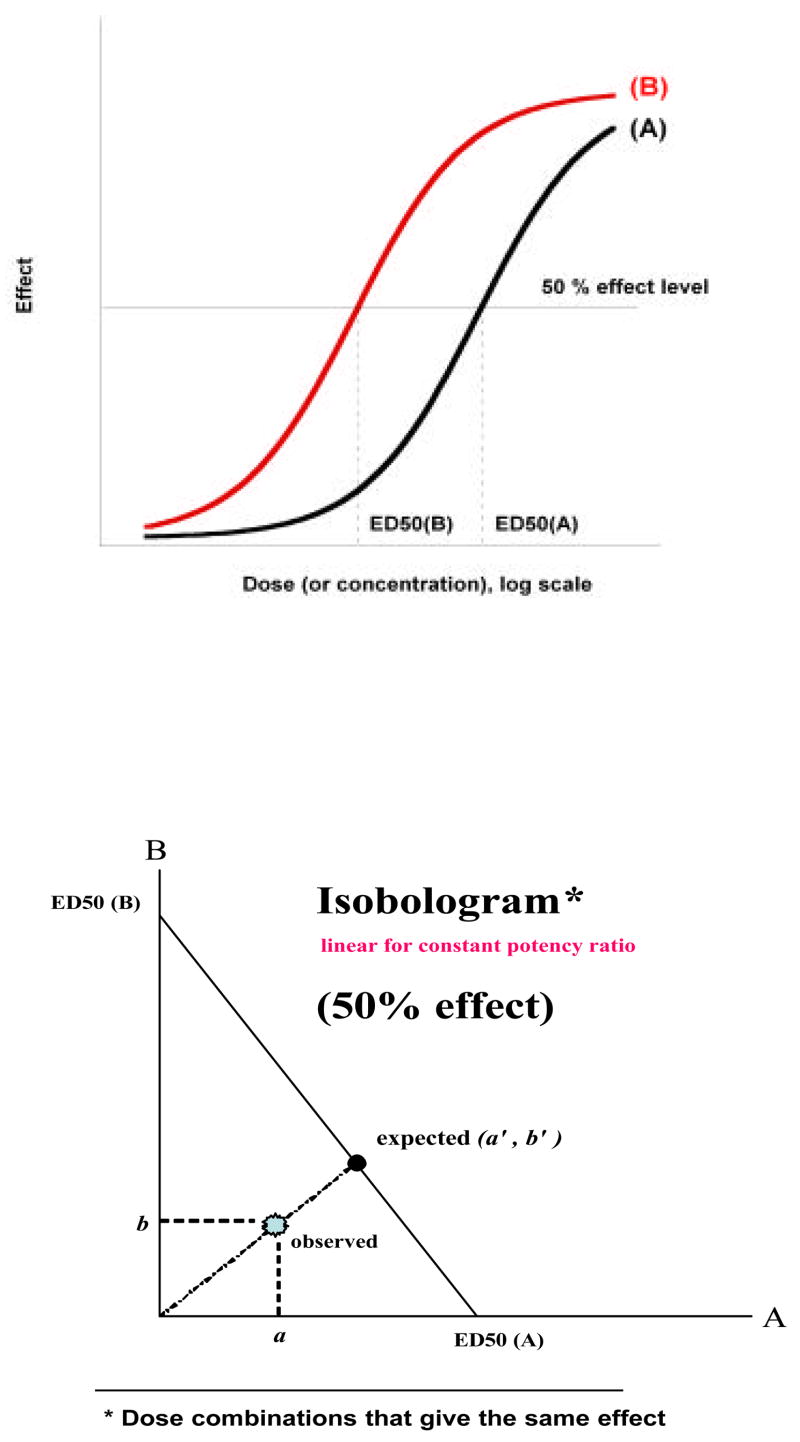
Fig.1.

(upper) Drugs with a constant potency ratio from which ED50 values are determined and plotted as shown in the lower graph in order to anchor the line of additivity. In this illustration a fixed-ratio combination that is additive would be on the line at point (a′,b′) while the experimental point has coordinates (a,b) so that it is below the line of additivity. The ratio of radial distances of point (a,b) to point (a′, b′) is the interaction index.

Experimental points (dose pairs) may be either on the expected curve or off it. The experimental isobole is found by determining the actual doses that give the specified effect and these dose pairs are plotted as points (dose combinations (a,b)) that give that effect. When the individual dose-effect curves show a constant relative potency, i.e., dose A/dose B = constant at all effect levels, then the expected isobole is linear (Fig. 1b).

This linearity is based on the concept of “additivity” as used in the early work of Loewe and most clearly expressed in (Loewe, 1953). This term follows from the concept of dose equivalence which means that a quantity of drug A is equivalent to some dose of drug B and, therefore, that equivalent can be added to the actual quantity of drug B to give a total equivalent of drug B. The latter quantity can then be applied to the dose-effect relation of drug B in order to determine the expected effect. In this case of constant relative potency the drugs A and B can be interchanged, i.e., the same procedure can be applied to get the quantity of drug B that is equivalent to the dose of drug A, so that its dose-effect relation provides the expected effect. In either case the same line results. Detail is provided in section 1.3. In a subsequent section (1.5) it is shown mathematically why the isobole of additivity is linear for drugs with a constant potency ratio but is curvilinear when that ratio varies with the effect level.

Two full agonists with a constant potency ratio will yield parallel log dose response curves as shown in Fig 1(a). From these one can determine the individual doses for a specified effect such as 50% of the maximum. In quantal (all or none) dose-effect relations these are ED50 doses. The additive (zero interaction) dose pairs are the points on the line with intercepts defined by each drug’s ED50. If, as illustrated, the experiment produces a point (dose pair) that gives the effect with doses less than those expected from the line, there is synergism (superadditivity) and the experimental point representing the actual dose pair lies below the line of additivity. The degree of synergism can be expressed as the interaction index (Tallarida, 2002), the ratio of the radial distances of the experimental point to the radial distance of the expected point on the line. Equivalently, the index is the ratio of the experimental total dose to the additive total dose (on the line). This metric allows a distinction between the expected and the exaggerated effects of a combination. This distinction is most readily made from a statistical analysis of the difference between the experimental total dose and the additive total dose. That analysis is contained in Tallarida (1992) and was further simplified (Tallarida, 2000) to yield approximate variances for use in a t-test that distinguishes between the additive and the experimental total doses. The calculations in the latter reference have also been incorporated into the software package PharmToolsPro (McCary Group, Emmaus PA, 18049).

Obtaining this metric can be an important first step in exploring mechanism. Essentially it tells us that there is something more to examine mechanistically. But even when this measure does not lead to an unraveling of mechanism, the detection of synergism and its degree is important as a guide to new experimentation and in furnishing useful clinical information. The statistics used in this analysis have been discussed in related works (Tallarida, 1992; 2000; 2006). This author’s experience suggests that minor departures from additivity, even when confirmed statistically, are likely to be not too convincing (and useful) to most investigators, i.e., such departures should be clearly evident and the statistical analysis merely confirmatory.

1.3 Dose equivalence

The concept of dose equivalence is the basis for distinguishing an exaggerated effect of a drug combination from a simply additive effect. When two drugs are present together it is not the effect of each that is added. In this section we discuss and illustrate what it is that is added and how that leads to the isobole as introduced by Loewe. The idea is aided by figure 2 which shows dose-effect curves for two agonists denoted here as drug (A) and drug (B). In this illustration no assumption regarding the maximum effects of each is made. The 50% effect level is indicated by the horizontal broken line and it shows the dose of drug B alone that is required to give this effect (B₅₀). The combination dose (a,b) that gives this effect consists of the quantity a that is equi-effective to some dose of B (denoted b_eq) plus the actual dose b in a quantity such that b_eq + b = B₅₀. Thus, dose b and b_eq are added, and it is this fact that gives rise to the term “additive” for this case. When the potency ratio is a constant, ℛ = dose(A)/(B), the b-equivalent of dose a is simply a/ℛ and, thus, b + a/ℛ = B₅₀, which yields equation (1) below that describes the linear isobole of additivity. This is a straight line in the first quadrant of a Cartesian coordinate system whose axes represent doses (or concentrations) of the two agents.

Fig.2.

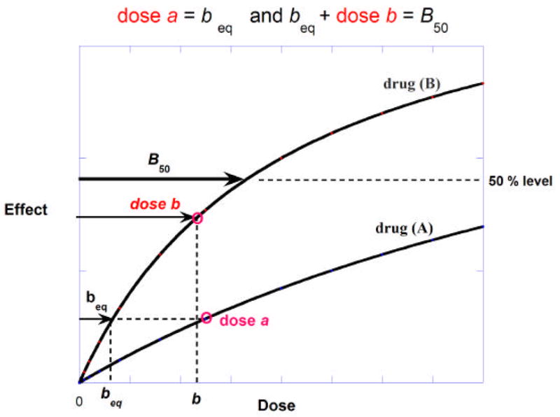
Illustration of dose equivalence for two drugs whose curves of effect against dose are shown and for which the maximum effects are not necessarily equal. The dose of drug A, denoted a, is found to be equi-effective to a dose of drug B that is denoted b_eq. That equivalent (b_eq) + the actual dose b add to give B₅₀ and, hence, the 50% effect. The set of (a,b) values constitute the isobole of additivity which is a straight line only if the potency ratio is constant at all effect levels.

$$\frac{a}{A_{50}}+\frac{b}{B_{50}}=1$$ (1)

In this case of constant potency ratio the same equation results if one adds dose a and the equivalent of drug A in terms of drug B, i.e., a + b ℛ, and equates that sum to A₅₀. It is seen, therefore, that this well-known relation whose graph is the familiar linear isobole is a consequence of dose equivalence as described here; it is not an empirical fact. This derivation also shows that the application of dose addition implies that the two drugs are assumed to be independent, i.e., not in competition for a common receptor.

There is an isobole of additivity for every effect level less than the maximum (E_max). When the potency ratio is constant these are parallel lines as shown in Fig. 3. For any effect level chosen, say an effect equal to some fraction C of the common maximum (C = E/E_max,) the additive isobole given by equation (1) becomes equation (2) shown below. This equation is applicable only to cases in which both drugs have the same maximum and gives rise to the set of parallel straight line isoboles as in Fig. 3.

Fig.3.

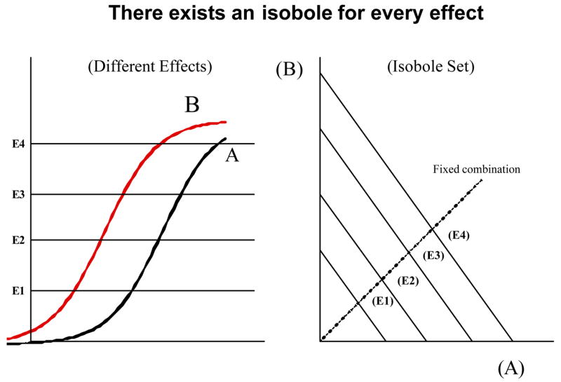
When the two drugs have a constant potency ratio their log(dose)-effect curves are parallel indicating a constant relative potency at every effect level and shown here(left) for four effect levels. For every effect level there is an isobole of additivity and these are linear and parallel (right).

$$\frac{a}{A_{50}\left(\frac{C}{1-C}\right)}+\frac{b}{B_{50}\left(\frac{C}{1-C}\right)}=1$$ (2)

For any choice of C < 1, equation (2) gives a line parallel to that defined by the 50% level (and for C = ½ it gives the 50% effect isobole).

If administration of a drug combination maintains a constant proportion of the constituents doses this will define a path that is radial from the origin as the combination quantity is increased. The intersection of this radial line with each isobole determines the dose combination that gives the effect of that isobole (Fig. 3). It is seen that the isobole computed from equation (1), or the form in equation (2), is clearly based on the concept of dose equivalence. This graph is not an empirical finding; the linearity follows from a basic assumption that the two compounds have a constant potency ratio or, equivalently, that their log(dose)-effect curves are parallel.

Many applications of this methodology have been made (including studies by this author) where the linear isobole of additivity is the basis for distinguishing departures from additivity. This usage carries with it the implicit assumption that the departure from parallelism of the constituent dose-effect curves is minor or relatively minor. A situation for which this assumption would not be justified is that in which the constituent drugs have obviously different maxima in the test situation. Therefore, most investigators have not applied the linear isobole of additivity to combinations of a full and a partial agonist, with certain exceptions. For example, when the second agent has very low efficacy, its dose can be downwardly adjusted to a zero effect level and this lowered dose can be used as a fixed amount along with graded doses of the efficacious drug to examine a combination effect. For example morphine was examined in combination with an ineffective (subantinociceptive) dose of the delta agonists, [D-Pen2, D-Pen5]enkephalin (DPDPE), [D-Ala2, Glu4]deltorphin in the mouse warm water tail flick test (Horan et al, 1992). When the second drug is truly lacking in efficacy (i.e., at all doses) then the standard analysis can be used. This situation is discussed next.

1.4 Analysis when one drug lacks efficacy

There are situations in which one of the two drugs in the combination lacks efficacy. In this situation the isobole of additivity for any specified effect is a horizontal line whose elevation is the dose of the active agent that produces the effect. In other words, an additive combination is independent of the dose of the inactive agent. In this situation it is easy to test for synergism or sub-additivity because the former is indicated by an experimental point that is below the horizontal line, while the latter, sub-additivity, is revealed by a point above the line. Equivalently, a significant lateral shift of the dose-effect curve of the effective drug when in the presence of the inactive drug would indicate a departure from additivity. An example of a situation of this kind occurs with antinociception (mouse abdominal constriction test) produced by ibuprofen in combination with glucosamine which has no analgesic efficacy in this test (Tallarida et al, 2003).

Another case of this kind, currently being investigated in collaboration with this author, involves the combination of a cannabinoid with MDMA (ecstasy) on body temperature Preliminary studies have shown that the cannabinoid, in a dose that has no effect on body temperature, reduces the hyperthermia produced by MDMA. (Presented as Thermoregulatory interaction between cannabinoids and MDMA K. Benamar, M. Yondorf, R.J. Tallarida, E. B. Geller and M.W. Adler, 2006, College on Problems of Drug Dependence).

The traditional method that employs the linear isobole of additivity is convenient because of its simplicity. In a test in which the individual dose-effect curves show reasonable parallelism, the method works well and generally allows a distinction between additive and non-additive interactions. The method has been helpful in making such conclusions from many drug combination experiments. A sampling of different applications of the method are contained in references cited in section 1.2. However, when the experimental points have been statistically determined to be off the line of additivity, but not too far off, then concern should be directed toward whether the assumption of a constant potency ratio is applicable. That constancy might be questioned either because the drugs produce different maximum effects or because there is a significant departure from parallelism in their log (dose)-effect curves. These two situations require the approaches that are discussed in the next sections.

1.5 Drugs that give different maximum effects

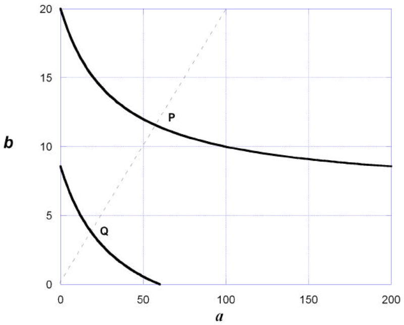
By definition, a full agonist and a partial agonist yield different maximum values and this is clearly a case of a varying potency ratio. In this situation the isobole of additivity is no longer a straight line but is curved (Grabovsky & Tallarida, 2004) as shown in Fig. 4. The theory underlying this curve is the same as that used in deriving the linear isobole, viz., the concept of dose equivalence is applied. To illustrate this, we use the common approach in which the dose-effect relations of the individual agents are modeled as hyperbolas. The effect E of each is a function of concentration: E = f(A) and E = g(B), where A and B are the respective concentrations. The functions are equated in order to derive the dose of drug A that is equivalent to a dose of drug B, and this leads to the additive isobole equation shown in equation (3) for effect level E_i. The dose of drug B, acting alone that gives this effect is denoted B_i. In discussing this topic the same notation used in the above-cited reference is employed. The full agonist gives the maximum effect, here denoted E_B, and is expressed in the concentration-effect equation given by E = E_B B/(B + B₅₀). The partial agonist is capable of producing effects up to E_C and is given by E = E_c A/(A + A_C). From these (and application of dose equivalence) the additive isobole for effect E_i is given by

Fig.4.

Additive isoboles for two different effect levels as described in the example are illustrated and are based on a full and a partial agonist in combination. The additive isoboles, calculated from Eq. (3), are curved because the relative potency of the two drugs is not constant but varies with the effect level. (See text example.)

$$b+\frac{B_{50}}{\frac{E_B}{E_c}\left(1+\frac{A_c}{a}\right)-1}=B_i$$ (3)

where B_i is the dose of drug B alone that gives effect E_i. Because E_c < E_B, the potency ratio is variable resulting in equation (3) which yields a curved isobole of additivity. (The common concentration-effect model used in deriving equation (3) leads to nonlinearity; however, the nonlinearity of the additive isobole is a consequence of the variable potency ratio and occurs regardless of the specific concentration-effect model). If the effect level selected is one that is attained by each drug when it acts alone then the isobole given by equation (3) will have intercepts on both axes. If an effect level is selected that is greater than that achieved by the partial agonist then the additive isobole will have no intercept on the dose-A axis; instead the curve decreases toward a horizontal asymptote. It may be noted that when both drugs have the same maximum, equation (3) becomes b + a ℛ = B_i, the common linear case discussed in section 1.3. A numerical example that applies equation (3) follows. An actual example, describing the combined action of a cannabinoid and an NMDA antagonist on body temperature (Rawls et al 2002), is discussed by Grabovsky and Tallarida (2004).

Example. In order to illustrate the application of equation (3) the following values are assigned: E_B (max of drug B) = 100, E_c (max of drug A) = 40, with constants, A_c = 20 and B₅₀ = 20. Isoboles of additivity for the 50 % effect level (which is not achieved by drug A alone) and for the 30 % effect are determined by use of equation (3). For 30 Bi the 50% isobole B_i is, of course, 20, while for the 30% isobole it is obtained from $\frac{30}{100}=\frac{B_i}{B_i+20}$ which yields 100 Bi + 20 B_i = 8.57. Thus, using equation (3) for the 50% level

$$b+\frac{20}{\frac{100}{40}\left(1+\frac{20}{a}\right)-1}=20$$

and for the 30 % effect level, B_i = 8.57, from which

$$b+\frac{20}{\frac{100}{40}\left(1+\frac{20}{a}\right)-1}=8.57$$

The two isoboles from this example are shown graphically in figure 4. A fixed-ratio combination will attain the effect levels shown at dose pairs represented by the intersection of a radial line that represents the constituent proportions in the combination (shown as broken line in Fig. 4). In the diagram these intersections are shown as points P and Q for a combination in which the constituent proportion (dose b: dose a) is 2:10. Intersection P is at (57.7, 11.5) and Q is at (18.8, 3.76). Therefore, a simply additive combination (zero interaction situation) would require dose combination Q for the 30% effect and dose combination P for the 50% effect.

It should be noted that fitting dose-effect data (D,E data) to smooth hyperbolic curves, e.g., E = E_max D/(D + C), or even to more complex curves, E = E_max D^p/(D^p + C^p) that contain the exponent p, is readily accomplished with many modern software packages, e.g., PharmToolsPro previously cited. These procedures use nonlinear regression to yield estimates of the curve parameters. Detailed discussions of nonlinear regression can be found in many standard works. This author’s monograph (Tallarida, 2000) discusses nonlinear regression with a focus on dose-effect data. Further, if curve fitting is not used, it is still possible to derive the isobole of additivity by the purely graphical method illustrated in figure 2. For the situations illustrated here the simple linear isobole is not applicable. However, it is replaced by a curve given in equation (3) that is only a bit more complicated. Besides the use of this equation for the situations illustrated here, it is shown in part II of this communication how this equation leads the way to a new application that numerically assesses the interaction between occupied receptors.

1.6 Two full agonists with a varying potency ratio

Besides the combination of a full and a partial agonist, another case of interest is that in which there are two full agonists with a varying potency ratio. This is exemplified by dose-effect curves whose equations include exponents (“Hill coefficients” p and q) as given in equations (4) and (5) below in which each attains the same maximum (E_max).

$$E=\frac{E_{max}{B}^p}{B^p+{B_{50}}^p}$$ (4)

$$E=\frac{E_{max}{A}^q}{A^q+{A_{50}}^q}$$ (5)

In this situation, termed “heterodynamic” by Loewe (1953), the application of dose equivalence leads to not just one, but to two additive isoboles when p and q are different. This duality arises because the drug A-equivalent of the dose of drug B, when added to dose a, is different from adding the drug B-equivalent of drug A’s dose to dose b. For effect level E_i, and respective potencies A_i and B_i, the two additive isoboles are given by the following (Tallarida, 2006)

$$b=B_{50}{\left(\frac{A_i-a}{A_{50}}\right)}^{q/p}$$ (6)

$$b=B_i-\frac{B_{50}}{{\left(\frac{A_{50}}{a}\right)}^{q/p}}$$ (7)

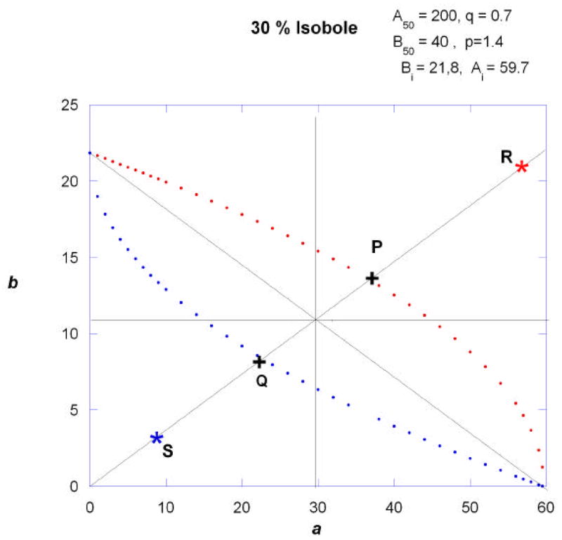
It has been shown mathematically (in the reference cited above) that in this case the two isoboles are symmetric with respect to the point (A_i/2, B_i/2). This symmetry is illustrated in the example shown in Fig. 5 for the 30% effect level, but it applies to all effect levels. Most often the effect level selected is 50% of the maximum. Each boundary curve represents additivity and, thus, the region contained between the two curves represents a region of additivity. If a combination containing these drugs is administered with a constant proportion of each constituent maintained in the combination the dose pairs plot as the radial line shown in Fig. 5. In this case an additive combination for this effect would lie somewhere along the segment indicated by points Q and P. A superadditive interaction would plot as point S and a subadditive interaction as point R.

Fig.5.

Isoboles of additivity for the 30% effect level are shown for two drugs that achieve the same maximum but have a potency ratio that changes with the effect, as indicated by different exponents p and q. In this illustration the 30% effect leads to A_i = 59.6, B_i = 21.8. The curves of additivity, calculated from equations (6) and (7), are symmetric with respect to a point at (A_i/ 2, B_i/ 2), in this case (29.8, 10.9).

Loewe certainly recognized that heterodynamic combinations have two isoboles for the same effect level (Loewe, 1953), and illustrated this phenomenon with figures in that paper, but this fact appears to have been not appreciated by investigators using the isobologram for analysis. This may be due to the metaphorical descriptions that Loewe used in an attempt to illustrate with three dimensional plots (effect plotted vertically above points in the plane that represent dose pairs) that he likened to sails on a boat. Further, Loewe, did not provide a formal mathematical exposition and did not examine or discuss the symmetry noted above. But his metaphors such as “sagging sail” and “inflated sail” are completely consistent with the mathematical descriptions given here.

With reference to figure 5, the sum of the coordinates at points P and Q, representing the total dose at each point, are readily determined. If an experimental value is obtained that appears to be sub-additive (such as point R) then the sum of its coordinates should exceed the sum at point P. The sum of the coordinates at P which is an upper value for additivity can be statistically compared to the sum at R (e.g., a one-sided t-test). Similarly, an experimental point such as S will be super-additive if the sum of its coordinates is less than the sum of the coordinates at Q.

1.7 Opposite effects

Most applications of isobolar analysis have involved drugs that produce similar effects. Yet there are situations in which the individual agents produce measurable dose-related effects that are in the opposite direction. This situation is exemplified when the effect is locomotive and also would apply when one compound increases body temperature and the other decreases the temperature. An example of the latter situation is afforded with lipopolysaccharide (LPS), which induces fever, whereas certain cannabinoids produce hypothermia (Rawls et al, 2002). Benamar et al from the laboratory of MW Adler examined this situation (presented in preliminary form at the College of Problems on Drug Dependence, 67 Ann. Meeting, Orlando FL, June, 2005) by the use of a cannabinoid + LPS combination in male Sprague Dawley rats. The cannabinoid employed was (+)-WIN 55,212-2 [(4,5-dihydro-2-methyl-4(4-morpholinylmethyl)-1-(1-naphthalenyl-carbonyl)-6H-pyrrolo[3,2,1ij]quinolin-6-one]. From the individual compound’s dose-response data, the doses that were effective in producing temperature changes of the same magnitude (but opposite in direction) were determined and subsequently administered together to a second group of animals. The result was a null effect, i.e., no significant change in body temperature, thereby suggesting that the concept of dose equivalence can be applicable even to cases in which the effects are in the opposite direction. In this case, the finding of no change in core temperature is consistent with simple additivity.

II. Multiple receptors: An extension of isobole theory

2.1 Introduction

Isobolographic methodology is not restricted to applications involving two or more distinct chemical entities or drugs. For example it has been applied to interactions in situations in which the same drug is administered at two different anatomical sites. Yeung and Rudy (1980) applied isobolographic analysis to experiments with morphine administered at both spinal and supraspinal sites while Raffa et al 2000 used a similar approach in examining the analgesic action of acetaminophen. A further extension of this approach, given here, is to an analysis of the action of a single drug that combines with two or more receptor types, a topic that constitutes part II of this review. Numerous studies in recent years have demonstrated that many classic receptors exist as several subtypes, e.g., three main opioid receptors, cholinergic muscarinics with five subtypes and dopaminergic with at least five. It is therefore possible and important to examine quantitatively the interactions between the several subtypes when they are occupied by the same drug or ligand. Genomic advances that have produced knockout animals, coupled with several methodologies for measuring receptor affinities, now provide opportunities to measure interactions among occupied receptors. A procedure for measuring such interactions follows from the concepts and illustrations in part I of this review.

The aim of this discussion is to illustrate the quantitative aspects and, in so doing, also provide a guide to (new) experimental designs that are needed to obtain the data. Applicable data from the laboratories of this author are used in the illustrations that follow. In analyzing these the common models of receptor binding have been used, e.g., those described in the guide of the National Institutes of Health Chemical Genomics Center (NCGC), a center established by NIH to create a national resource in chemical probe development that also includes methodology useful in the study of knockout animals that retain the receptor types of interest.

The approach to studying interactions between occupied receptors begins with the dose-effect data from both the wild type and the requisite transgenic animals (or animal parts) that lacks certain receptors. For example, consider a system with two receptors that are here referred to as R₁ and R₂. It is assumed that each contributes to the effect when an agonist drug is administered to the wild type. Concentration-effect data from the R₁ knockout yield data due to agonist action at the R₂ receptor whereas the data from the R₂ knockout yield agonist action mediated by R₁. Affinity values (1/K_D) for the individual receptor subtypes and drug concentration [A] lead to the fractional receptor occupation by application of mass action: [A]/([A]+K_D). Thus, the three curves of concentration-effect data are obtained; one set from R₁ knockouts, another from R₂ knockouts and a third from the wild type containing both. The concentration-effect curves lead to occupation-effect curves for the three cases. An isobole of occupation is then determined using equation (3) which was previously derived for application to situations that give different E_max values. In this application the concentration terms and associated constants in that equation are replaced with fractional occupations of the two receptors and the constants in the concentration effect relation are replaced by the corresponding constants obtained (by nonlinear regression analysis or as subsequently described) from the occupation-effect data of each receptor. Details are illustrated in the following examples.

2.2 Examples: Interaction between occupied receptors

Occupation Isoboles: Example 1

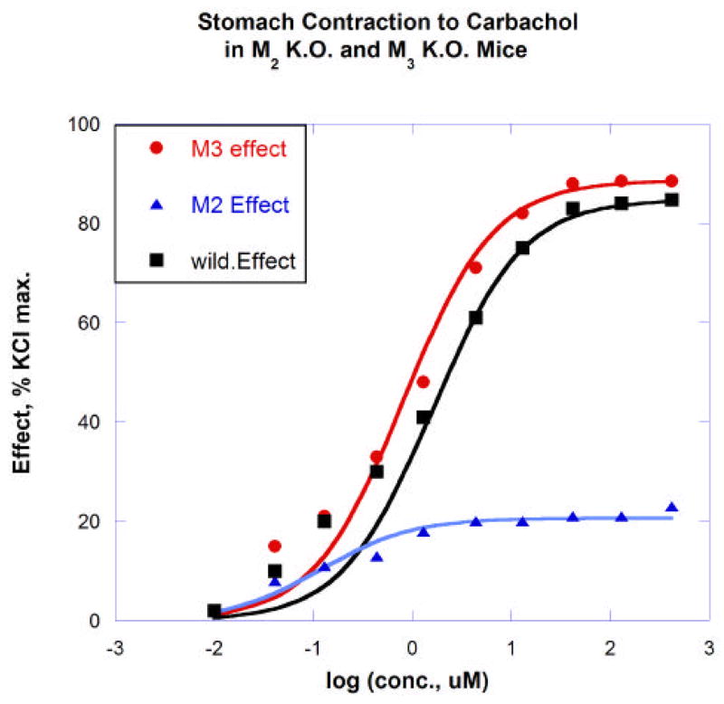
The illustration provided here uses data from ongoing studies in our laboratories (in collaboration with M. Ruggieri). These experiments examined carbachol (carbamolylcholine)-induced contraction in isolated mouse stomach muscle from wild type and from muscarinic M₂ and M₃ knockout mice. These two receptor sub-types were determined to be the ones that contribute to the development of carbachol-induced tension in this preparation. The graphs below (Fig 6) show the concentration-effect relations for this agonist on tissue from M₂- and M₃- knockouts and from the wild type. Although the aim here is to illustrate the calculation procedures and the associated experimental designs needed to produce the data, it is nevertheless desirable to use realistic values of drug parameters, i.e., K_D values that have the appropriate order of magnitude. Toward that end this example uses generally accepted high affinity of carbachol for the cholinergic M₂ receptor (K_D = 2.75 uM) and lower affinity for the M₃ (K_D = 62 uM), values obtained from the PDSP K_i database, (Psychoactive Drug Screening Program, a resource that provides parameter values and screening of compounds for pharmacological and functional activity at cloned human or rodent receptors.) These K_D values permit a calculation of the receptor occupancy from standard mass-action binding, [A][R_t]/([A] +K_D) for a drug in concentration [A] and total receptor concentration [R_t]. Division by [R_t] gives the fractional binding. (This calculation of binding and the other receptor binding formulas used in subsequent parts of this communication are the most common mass-action binding models and are concisely summarized in the guide of the NCGC). These are quite suitable to illustrate the calculations for this analysis which is the main objective here. To provide a further examination, following this first example, it is shown in a second example how the use of a different pair of parameters (dissociation constants) would affect the results.

Fig. 6.

Dose response curves in mouse isolated stomach muscle for carbachol in wild type and in M2 knockout (M3 effect) and M3 knockout (M2 effect).

Concentration-effect values were transformed to (fractional) receptor occupation-effect values using the K_D values for carbachol as noted above (K_D = 2.75 uM and 62uM). From these and the application of nonlinear regression, the following occupation-effect relations were derived:

$$E=21.62\hspace{0.17em}[{\text{M}}_2]/([{\text{M}}_2]+0.0459)$$ (8)

$$E=88.56\hspace{0.17em}[{\text{M}}_3]/([{\text{M}}_3]+0.0128)$$ (9)

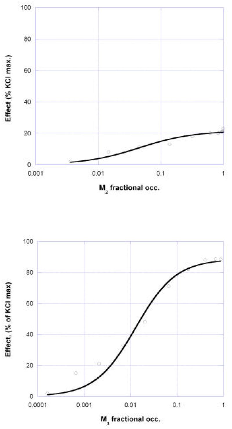
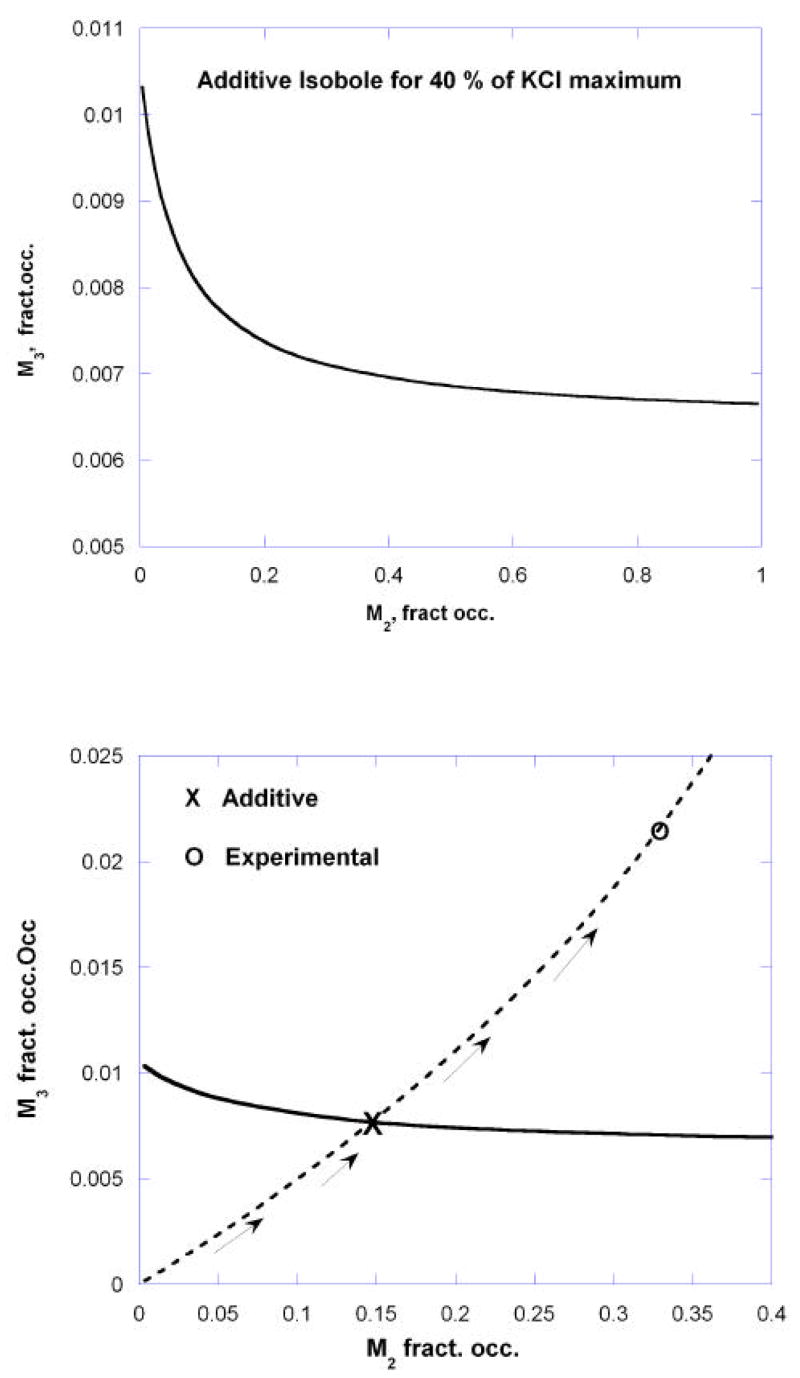
where [M₂] and [M₃] denote the fractional occupation of M₂ and M₃ receptors, respectively. (A simple method for converting a concentration-effect equation into the appropriate occupation-effect equation is given in the appendix.). Graphs of these are shown in figure 7. These two very different occupancy-effect relations show clearly that the ratio of potencies based on receptor occupation vary considerably with the effect level so that the usual linear isobole would not be applicable. This case requires the use of equation (3) which was derived from dose equivalence for drugs that show this variability, and is applied here where the independent variable is the fractional receptor occupation. From the two occupation-effect relations (equations (8) and (9)) the isobole of additivity is obtained by using equation (3) where the concentrations in that equation are now replaced by the occupation fractions for the two receptors. Selected for illustration here is the isobole of additivity for the effect = 40% of the KCl maximum, a level approximately in the middle of the range for carbachol in the M₂ knockout animal. This effect is not attained by M₂ agonism but is reached by the M₃ (in the M₂ knockouts) at fractional occupation = 0.01055 uM. Substitution of values from (8) and (9) in equation (3) is as follows: E_B = 88.56, E_C = 21.62, A_C = 0.0459 and B₅₀ = 0.01281. Using these in equation (3) yields the additive occupation isobole shown as equation (10) for the receptor pair and illustrated in the graph of Fig. 8.

Fig.7.

Occupancy-effect relations for M₂ fractional occupation (from M₃ knockouts) and M₃ occupation (from M₂ knockouts) for carbachol-induced contraction of isolated stomach muscle in mouse.

Fig.8.

Isobole for effect = 40% KCl maximum as determined from the fractional occupation of M₃ and M₂ cholinergic receptors by carbachol in mouse stomach muscle The lower graph, with adjusted scales, shows the occupation path and its direction as the carbachol concentration is increased in the wild type. The experimentally derived point is seen to be clearly above the additive point, thereby indicating a sub-additive interaction when both muscarinic receptors are occupied.

$$[M_3]=0.01055-\frac{0.01281}{3.0962+\frac{0.188}{[M_2]}}$$ (10)

This isobole is also shown with different scales in Fig. 8 (lower) in order to illustrate the changing occupation of the M₂ and M₃ receptors (shown with broken lines) that corresponds to increasing carbachol concentration. The intersection of this occupancy “path” with the additive isobole occurs at [M₂] = 0.1476, [M₃] = 0.0076, values which correspond to carbachol = 0.476uM. This means that the combination occupation of these receptor subtypes, as in the wild type that contains both, is expected to require 0.476 uM to achieve the 40% effect level if there is no interaction. However, the carbachol concentration actually required to achieve this effect is 1.40 uM (Fig. 6), a value approximately three times greater than the concentration that is expected from additivity. Stated differently, the fractional occupancies actually required are at occupancy point (0.337, 0.0221) as shown in Fig. 8 (lower). This result is indicative of an appreciable sub-additive interaction between these receptor types in the wild type preparation. A measure of that sub-additivity is indicated by the ratio of the actual to the additive carbachol concentrations, 1.40/0.476 = 2.94.

Occupation Isoboles: Example 2

A second example is provided in order to illustrate how the use of a different pair of dissociation constants for this same agonist at M₂ and M₃ would affect the analysis. The value of K_D used in this second example is 30 μM for both receptor sub-types, a value listed by Eglen and Whiting (1987) that was obtained by using a standard pharmacological method (Furchgott, 1966; Furchgott & Bursztyn, 1967) that is based on a single receptor type. Thus, 30 μM is taken to be a measure of the affinity for both receptors in this second example. This choice of constants leads to the occupation-effect relations shown graphically in Fig. 9 (upper) and the additive isobole shown in the lower plot. The lower plot shows a straight line path for the dual receptor occupation in this case because the K_D values are the same. As found in the first example this case also shows sub-additivity. The additive point (intersection coordinates of both = 0.0155) corresponds to a carbachol concentration = 0.473 uM, approximately the same as in the first example; thus, the measure of interaction as the ratio of the actual concentration to the additive concentration is 1.40/0.473= 2.96, a value quite close to that of the first example. The agreement between this and the first example is striking, even though the equal K_D values used here are rather different than the values (2.75, 62) used in the first example. (The methodology is sufficiently robust that even a major change in the K_D values assigned, e.g., a reversal of affinity magnitudes to K_D = 5 for M₃ and 40 for M₂, also shows sub-additivity (from a calculation not shown here) and with an agonist ratio 1.40/0.448 = 3.13, a value that is not too different from the value from example 1).

Fig. 9.

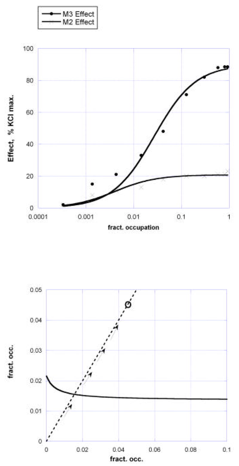
(Upper) Occupation-effect curves for the M₃ receptor, given by E = 89.8 [M₃] / ([M₃] + 0.0268), and for the M₂ receptor by E = 20.75 [M₂] / ([M₂] + 0.00404) as described in Example 2. (Lower) shows the additive isobole for the 40% effect and also shows the occupation path (broken line). The experimental occupancy point (O) is seen to be appreciably above the intersection of the curves.

2.3 Competitive inhibition in the dual receptor case

A competitive antagonist with affinity for one or both receptors will reduce the occupation of the agonist and, thus, reduce its effect. Restoration of the agonist’s effect requires increasing its concentration. But in this dual receptor case the restoration accompanying increased agonist concentration is to an occupancy point on the occupation isobole. If the interaction is additive, that isobole is the isobole of additivity. If the interaction is not additive, then restoration of the effect is to a point on the applicable non-additive isobole that is determined by experiment. This stands in contrast to the one-receptor model of competitive antagonism which assumes that effect restoration means a return to the agonist occupation before the block. (That single receptor model is the basis of the Schild Plot discussed subsequently). Continuing the discussion with the two muscarinic receptor types and the values in example 1, effect restoration now means a return to some point on the carbachol occupation isobole. Fig. 10 illustrates as it shows the occupation paths for increasing carbachol concentration in the presence of a competitive blocking drug, in this case, 10 nM atropine. This same figure also shows the path in the absence of the competitor. The agonist fractional occupation in the competitive case is determined from the familiar relation, introduced by Gaddum (1937), widely applied and given by, [A]/([A] + K_D (1+[B]/K_i), where [B] is the competitor concentration and K_i is its reciprocal affinity for the receptor in question. This illustration used the K_i values for atropine that are given in the legend of figure 10. Of course, the M₂–M₃ occupation pairs for increasing carbachol in the presence of the blocker are different from the pairs in the unblocked case and the graph shows both. This graph also shows intersections as points labeled 1 and 2 that would apply if the interaction between M₂ and M₃ were additive. Point 1 is the previously determined point for additivity for carbachol alone, whereas point 2 (0.367, 0.007) shows the point of return for increasing carbachol in the presence of a fixed concentration of the blocker. This point corresponds to carbachol concentration = 14.2 uM and would be the required concentration to restore the effect in the additive case. Because the interaction between M₂ and M₃ was shown to be sub-additive, the actual restoration of the effect is to some point beyond point 2 along the path shown. (Experiments are currently underway in our laboratories to determine this point, and other points that apply for several different concentrations of this and other cholinergic blocking drugs.) A further examination of competitive inhibition in this two receptor situation is included in the next section on the Schild plot.

Fig. 10.

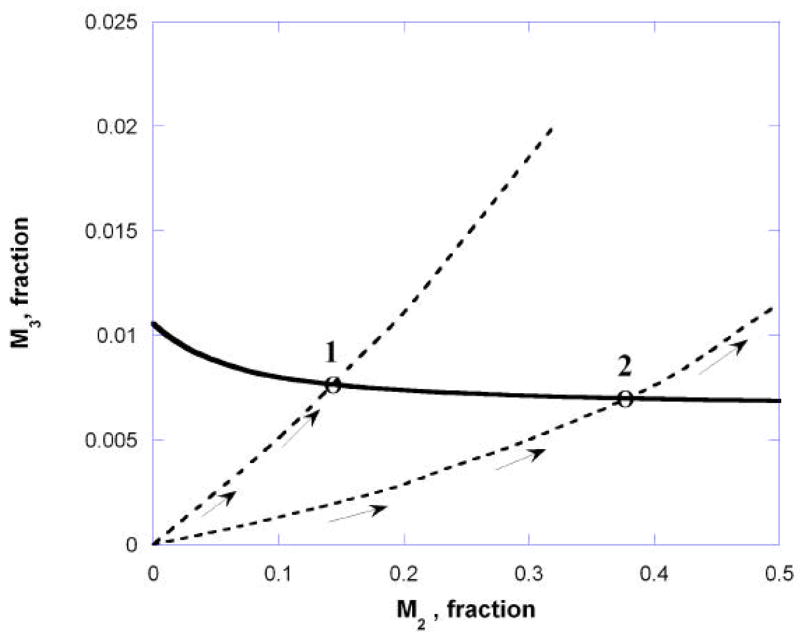
Shown is the isobole of additivity for the 40% effect (solid curve) and the carbachol occupation “paths” under two different conditions. The paths indicate the simultaneous carbachol occupation of the M₂ and M₃ receptor for increasing concentration when it is the sole drug (upper broken curve) and when atropine is present in a fixed concentration = 10 nM (lower broken curve). Point 1 shows the additive occupation pair in the absence of the antagonist, while point 2 is the carbachol additive occupation pair that would restore the effect level when the antagonist is present. This illustration used the atropine mouse smooth muscle dissociation constants 1.26 nM at M₂ and 0.316 nM at M₃ (Choppin & Eglen, 2001).

2.4 Schild plot

An analysis of competitive antagonism by Schild (1947) ultimately led to a graph bearing his name that has been widely applied for determining the affinity of a competitive antagonist (Arunlakshan & Schild, 1959). The Schild plot follows from the single-receptor model in which the competitive antagonist (dissociation constant K_B) is administered in concentration [B] following the determination of an agonist’s concentration-effect relation for increasing concentrations [A] of the agonist whose dissociation constant is K_A. The model is based on a single receptor type present in concentration [R_t]. The presence of the antagonist reduces the agonist occupation [AR] from [A][R_t]/( [A] + K_A ) to the lesser concentration [AR]* given by

$$[AR]\ast =\frac{[A][R_t]}{[A]+K_A(1+[B]/K_B)}$$ (11)

This reduction in agonist receptor occupation results in an associated reduction in the effect of the agonist. Restoration of that effect level therefore requires a greater concentration of agonist to some value [A]′in order to produce the original agonist occupation, and this leads to the relation [A]′/[A] =1 + B/K. In most experiments the B agonist concentration-effect curve is determined in the presence of several different fixed concentrations [B] and the dextrally shifted curves give [A]′for each [B]. Rearrangement of this equation to logarithmic form gives Log ([A]′/[A] − 1) = Log[B] − Log(K_B) and thus, a plot of Log ([A]′/[A] −1) against Log [B] is linear for increasing concentrations [B], with slope one and vertical intercept = −Log (K_B). This plot is the well-known Schild plot and its intercept gives the negative logarithm of the antagonist dissociation constant. When concentrations (and K values) are in molar units the intercept is termed “pA₂.” In practice, the slope is seldom exactly unity in which case the intercept on the abscissa (multiplied by minus one) is reported as the pA₂. Departures from unit slope and from linearity of the plot may be due to the scatter of the data or uncertainty in the values of concentration in the immediate receptor environment. More likely these are due to more basic assumptions in this derivation that are not applicable in many experiments. One assumption has to do with simple mass-action binding as opposed to more complex binding. A more glaring assumption is that the Schild plot is based on competition for a single receptor type. It is therefore instructive to examine Schild analysis in a system in which two or more receptors mediate the effect of the agonist.

2.5 Competitive inhibition with two receptors and the “pA₂”

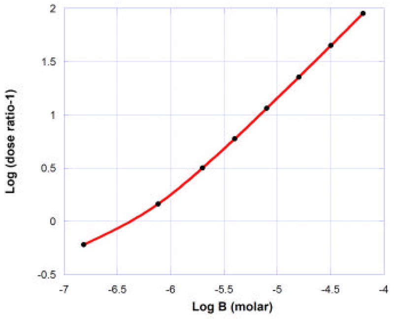
If the interaction between the two receptors is additive then the presence of a fixed concentration of an antagonist should restore the unblocked effect when the occupation path defined by increasing agonist reaches the agonist’s occupation isobole. In Fig. 10 this was shown as point 2. The path leading to this intersection is determined from the pair of agonist dissociation constants at the receptors (K_A2 and K_A3 for the M₂ and M₃ receptors, respectively) and from the antagonist pair at these receptors (K_B2 and K_B3). (The appendix provides further mathematical details.) Unlike the traditional concentration-based isoboles in which the experimenter can control the doses, the path for increasing agonist in the occupation-based isobole is defined by these four K values and the antagonist concentration [B]. The use of different [B] values yields different paths and hence different intersections with that isobole (e.g., to the right or left of point 2 of figure 10, depending on [B]). Each point of intersection gives the agonist occupation and, hence, the agonist concentration [A]′ needed to restore the (additive) effect, and these, along with their corresponding [B] values, are precisely the quantities used in the Schild plot. It is therefore possible to determine what the Schild plot becomes with two receptors in a situation of zero interaction (pure additivity). One such outcome is illustrated in figure 11 for an antagonist that has preferential affinity for the M₂ muscarinic receptor. The slight curvature seen is consistent with the choice of the four K’s (carbachol as in example 1, but K_B2 = 0.01 and K_B3 = 1000 for the antagonist).

Fig. 11.

Illustration of a Schild plot for carbachol with an antagonist having high affinity for the muscarinic M₂ receptor in isolated mouse stomach. (See text). Nonlinearity, though slight, is evident. When the points were fitted to a straight line the slope = 0.850 and the pA₂ = 6.39.

Additional insight is gained from a further examination of competitive inhibition of carbachol with antagonists that have preferential affinity for one or the other receptors used in this example. Table 1 shows the results of calculations based on additivity when the antagonist has assigned preferential affinity for the M₃ receptor (i.e., K_B3 small and K_B2 large) and when the opposite situation prevails. Note that when K_B3 is small the block is at the dominant receptor (the M₃), a situation closer to the one-receptor model. In this case the Schild plot slope is near unity and the apparent K_B value derived from it approximates the value of K_B3. In contrast, when K_B2 is small so that the block is at the less dominant receptor, the Schild plot slope is < 1 and the K_B value derived from the pA₂ lies between K_B2 and K_B3.

Table 1.

Schild plot results for carbachol with various antagonist dissociation constants (K_B2 and K_B3, nM) at muscarinic M₂ and M₃ receptors if the interaction were additive. The agonist dissociation constants were fixed at the values used in example 1, viz., K_A2 = 2.75 and K_A3 = 62.0 (nM) whereas the antagonist K’s are varied as indicated. For each of the four cases shown a Schild analysis was made in the usual (linear) way, thereby providing the line’s slope and pA₂ value. The apparent K listed in each case is the antagonist dissociation constant (nM) calculated from the derived pA₂.

KB2	KB3	Slope	pA2	Kapparent
0.1	100	0.854	7.38	41.7
1.0	100	0.881	7.33	46.8
100	0.1	1.00	9.94	0.115
100	1.0	0.999	8.94	1.15

2.6 Summary

The isobolographic method of Loewe is rooted in the concept of dose equivalence. When applied to two agonists whose relative potency is constant over the effect range the isobole of additivity yields the familiar linear graph. But, when the relative potency is variable, a situation most evident when the drug pair is a full and a partial agonist in eliciting the effect of interest, the application of dose equivalence gives rise to an additive isobole that is curvilinear and given by equation (3). Two full agonists that display log dose-effect curves that depart significantly from parallelism also yield curvilinear isoboles, but these have a symmetry with respect to a point in their midrange and are calculated from equations (6) and (7). Historically most applications of isobolographic analysis have used the linear isobole as the basis for distinguishing between additive and non-additive interactions. Thus, most users of this technique (including this author) have either demonstrated sufficient similarity in the constituent dose-effect curves that lead to linear isoboles or judged the departures to be minor. This practice is somewhat understandable because linearity is simple and convenient for analysis. However, the curvature, when it has to be applied, is really not very complicated (as seen by equation (3)) and, in this era of widespread computer usage, the application of the needed equation should not limit the use of isoboles in drug combination studies.

The recognition that drugs of different efficacy lead to nonlinear isoboles means a different (though simple) calculation is required, but this recognition and the use of the applicable equation has led to an interesting expansion of their use, viz. to the occupation of receptor subtypes for a single drug. This situation (now well accepted) refers to the observations that many individual agonists produce effects that are mediated by more than one receptor. In this case the use of equation (3) is applicable to the individual receptor occupation and is actually required because the maximal effects due to each receptor acting alone will likely be rather different, thereby necessitating a change from the linear isobole. This difference in E_max was clearly shown for the two muscarinic cholinergic receptors described in this communication. Similar differences are known for other drugs and drug classes, e.g., opioid receptors mediating the analgesic effects of morphine. As experimentation with transgenic animals and animal preparations continue to proliferate there will likely be many more examples of receptor sub-types displaying different intrinsic activities for the same agonist. The generalization of the isobole calculation to apply to two drugs of different efficacy has led to the extension of the method to the multi receptor application described here. This application, in turn, has provided a measurement of the interaction between these receptor types and has also given new insights on the quantitation of competitive antagonism and the interpretation of the classic Schild plot. While the examples used in this review illustrated effects from two occupied receptors, the results are readily generalized to multiple receptor sub types. The material in this review signals the need for certain new experimental designs that may aid in furthering our understanding of single and multiple drug action.

APPENDIX

1. Transformation of concentration-effect relation to occupation-effect relation

When the agonist concentration effect data ([A], E) have been fitted by nonlinear E_max [A] regression to the usual hyperbolic form given by $E=\frac{E_{max}[A]}{[A]+C_A}$, this equation may be transformed to fractional receptor occupation, $X=\frac{[A]}{[A]+K_A}$ as required for certain applications discussed in this paper. The transformed equation has the form $E=\frac{E^{\prime }X}{X+\gamma }$. Since the two expressions for E are equal for any value of [A], equating these yields $E^{\prime }=\left(\frac{K_A}{K_A-C_A}\right)E_{max}$ and $\gamma =\frac{C_A}{K_A-C_A}$. Therefore, a second nonlinear curve fit is not necessary to get the occupation-effect equation.

2. Determining the path representing the simultaneous occupation of an agonist by two receptors

The dissociation constants for the M₂ and M₃ receptor for the agonist are here denoted by K_A2 and K_A3, respectively, and for the antagonist, by K_B2 and K_B3. For varying agonist concentration [A] and a fixed concentration [B] of the antagonist, the agonist fractional occupation of the M₂ receptor is given by

$$[M_2]=\frac{[A]}{[A]+K_{A2}(1+[B]/K_{B2})}$$

and that of the M₃ receptor by

$$[M_3]=\frac{[A]}{[A]+K_{A3}(1+[B]/K_{B3})}.$$

The above allow a spreadsheet column of [A] values to be used in calculations from the above to yield corresponding columns for [M₂] and [M₃], thereby allowing construction of the graph of [M₃] against [M₂]. This process was employed for the graphs of paths in the main text. Alternatively, the above are parametric equations from which [A] can be eliminated to yield the path equation shown below:

$$[M_3]=\frac{K_{A2}(1+[B]/K_{B2})[M_2]}{K_{A3}(1+[B]/K_{B3})+\{K_{A2}[1+[B]/K_{B2}]-K_{A3}[1+[B]/K_{B3}]\}[M_2]}$$

References

- Arunlakshana O, Schild HO. Some quantitative use of drug antagonists. Br J Pharmacol. 1959;14:48–57. doi: 10.1111/j.1476-5381.1959.tb00928.x. [DOI] [PMC free article] [PubMed] [Google Scholar]
- Berenbaum MC. What is synergy? Pharmacol Rev. 1989;41:93–141. [PubMed] [Google Scholar]
- Bolan EA, Tallarida RJ, Pasternak GW. Synergy between mu receptor subtypes: Evidence for functional interaction among mu receptor subtypes. J Pharmacol Exp Ther. 2002;303:557–562. doi: 10.1124/jpet.102.035881. [DOI] [PubMed] [Google Scholar]
- Choppin A, Eglen RM. Pharmacological characterization of muscarinic receptors in mouse isolated urinary bladder smooth muscle. Brit J Pharmacol. 2001;133:1035–1040. doi: 10.1038/sj.bjp.0704165. [DOI] [PMC free article] [PubMed] [Google Scholar]
- DiFazio CA, Brown RE, Ball CG, Heckel CG, Kennedy SS. Additive effects of anesthetics and theories of anesthesia. Anesthesiology. 1972;36:57–63. doi: 10.1097/00000542-197201000-00010. [DOI] [PubMed] [Google Scholar]
- Eglen RM, Whiting RL. Estimation of apparent agonist affinity constants using desensitization of the ileal muscarinic receptor. J Pharmacol Exp Ther. 1987;240:404–409. [PubMed] [Google Scholar]
- Field MK, Gonzalez MI, Tallarida RJ, Singh L. Gabapentin and the NK1 antagonist CI-1021 act synergistically in two rat models of neuropathic pain. J Pharmacol Exp Ther. 2002;303:730–735. doi: 10.1124/jpet.102.033134. [DOI] [PubMed] [Google Scholar]
- Furchgott RF. The use of beta-haloalkylamines in the differentiation of receptors and the determination of dissociation constants of receptor agonist complexes. Advan Drug Res. 1966;3:21–55. [Google Scholar]
- Furchgott RF, Bursztyn P. Comparison of dissociation constants and of relative efficacies of selected agonists acting on parasympathomimetic receptors. Ann NY Acad Sci. 1967;144:882–893. [Google Scholar]
- Gaddum J. The quantitative effects of antagonistic drugs. J Physiol (London) 1937;89:7P–9P. [Google Scholar]
- Gershwin ME, Smith NT. Interaction between drugs using three dimensional isobolographic interpretation. Arch Int Pharmacodyn Ther. 1973;201:154–161. [PubMed] [Google Scholar]
- Gessner PK, Cabana BE. A study of the hypnotic effects and the toxic effects chloral hydrate and ethanol. J Pharmacol Exp Ther. 1970;174:247–259. [PubMed] [Google Scholar]
- Grabovsky Y, Tallarida RJ. Isobolographic analysis for combinations of a full and partial agonist: curved isoboles. J Pharmacol Exp Ther. 2004;310:981–986. doi: 10.1124/jpet.104.067264. [DOI] [PubMed] [Google Scholar]
- Horan P, Tallarida RJ, Haaseth RC, Matsunaga TO, Hruby VJ, Porreca F. Antinociceptive interactions of opioid delta receptor agonists with morphine in mice: Supra- and subadditivity. Life Sci. 1992;50:1535–1541. doi: 10.1016/0024-3205(92)90144-e. [DOI] [PubMed] [Google Scholar]
- Kimmel HL, Tallarida RJ, Holtzman SG. Synergism between buprenorphine and cocaine on the rotational behavior of the nigrally-lesioned rat. Psychopharmacol. 1997;133:372–378. doi: 10.1007/s002130050416. [DOI] [PubMed] [Google Scholar]
- Loewe S, Muischnek H. Uber Kombinationswirkungen. I. Mitteilung: Hilfsmittel der Fragestellung. Arch Exp Path Pharmakol. 1926;114:313–326. [Google Scholar]
- Loewe S. Die Mischiarnei. Klin Wochenschr. 1927;6:1077–1085. [Google Scholar]
- Loewe S. Die quantitativen Probleme der Pharmakologie. Ergebn Physiol. 1928;27:47–187. [Google Scholar]
- Loewe S. The problem of synergism and antagonism of combined drugs. Arzneimittelforschung. 1953;3:285–290. [PubMed] [Google Scholar]
- Miranda HF, Sierraita F, Pinardi G. Neostigmine interactions with nonsteroidal anti-inflammatory drugs. Br J Pharmacol. 2002;135:1591–1597. doi: 10.1038/sj.bjp.0704599. [DOI] [PMC free article] [PubMed] [Google Scholar]
- Masusda Y, Utsui Y, Shiraishi Y, Karasawa T, Yoshida K, Shimzu M. Evidence for a synergistic interaction between phenytoin and phenobarbital in experimental animals. J Pharmacol Exp Ther. 1981;217:805–811. [PubMed] [Google Scholar]
- Pircio AW, Buyniski JP, Ruebel LE. Pharmacological effects of a combination of butorphanol and acetaminophen. Arch Int Pharmacodyn Ther. 1978;235:116–123. [PubMed] [Google Scholar]
- Raffa RB, Stone DJ, Jr, Tallarida RJ. Discovery of ‘self-synergistic’ spinal/supraspinal antinoci-ception produced by acetaminophen (paracetamol) J Pharmacol ExpTher. 2000;295:291–294. [PubMed] [Google Scholar]
- Raffa RB, Friderichs E, Reimann W, Shank RP, Codd EE, Vaught JL, Jacoby HI, Selve N. Complementary and synergistic antinociceptive interaction between the enantiomers of tramadol. J Pharmacol Exp Ther. 1993;267(1):331–40. [PubMed] [Google Scholar]
- Rawls SM, Cowan A, Tallarida RJ, Geller EB, Adler MW. N- Methyl-D-aspartate Antagonists and WIN 55212-2 [4,5-Dihydro-2-methyl-4(4- morpholinylmethyl)-1-(1-naphthalenyl-carbonyl)-6H-pyrrolo[3,2,1-i,j]quinolin-6- one], a Cannabinoid Agonist, Interact to Produce Synergistic Hypothermia. J Pharmacol Exp Ther. 2002;303(1):395–402. doi: 10.1124/jpet.102.037473. [DOI] [PubMed] [Google Scholar]
- Rawls SM, Cowan A, Tallarida RJ, Geller EB, Adler MW. NMDA antagonists and WIN 55212-2, a cannabinoid antagonist, interact to produce synergistic hypothermia. J Pharmacol Exp Ther. 2002;303:395–402. doi: 10.1124/jpet.102.037473. [DOI] [PubMed] [Google Scholar]
- Schild HO. pA2, a new scale for the measurement of drug antagonism. Br. J Pharmacol. 1947;2:189–206. doi: 10.1111/j.1476-5381.1947.tb00336.x. [DOI] [PMC free article] [PubMed] [Google Scholar]
- Smith NT, Corbascio AN. Interaction between pentobarbital and decreased calcium ion in guinea pig atria. Anesth Analg Curr Res. 1966;45:576–581. [PubMed] [Google Scholar]
- Tallarida RJ, Cowan A, Adler MW. pA2 and Receptor Differentiation: A Statistical Analysis of Competitive Antagonism. Mini-review. Life Sciences. 1979;25:637–654. doi: 10.1016/0024-3205(79)90505-8. [DOI] [PubMed] [Google Scholar]
- Tallarida RJ. Statistical analysis of drug combinations for synergism. Pain. 1992;49:93–97. doi: 10.1016/0304-3959(92)90193-F. [DOI] [PubMed] [Google Scholar]
- Tallarida RJ. Drug Synergism and Dose-Effect Data Analysis (monograph) CRC/Chapman-Hall; Boca Raton: 2000. [Google Scholar]
- Tallarida RJ. Drug Synergism: Its Detection and Applications. Perspectives in Pharmacology (Invited Review) J Pharmacol Exp Ther. 2001;298:865–872. [PubMed] [Google Scholar]
- Tallarida RJ. The Interaction Index: A Measure of Drug Synergism. Pain. 2002;98:163–168. doi: 10.1016/s0304-3959(02)00041-6. [DOI] [PubMed] [Google Scholar]
- Tallarida RJ. Commentary on neostigmine interactions with non steroidal anti- inflammatory drugs by Miranda et al. Br J Pharmacol. 2002a;135:1589–1590. doi: 10.1038/sj.bjp.0704600. [DOI] [PMC free article] [PubMed] [Google Scholar]
- Tallarida RJ, Cowan A, Raffa RB. Antinociceptive Synergy, Additivity, and Subadditivity with Combinations of Oral Glucosamine Plus Nonopioid Analgesics in Mice. J Pharmacol Exp Ther. 2003;307:699–704. doi: 10.1124/jpet.103.054320. [DOI] [PubMed] [Google Scholar]
- Tallarida RJ, Cowan A, Raffa RB. Antinociceptive synergy, additivity, and subadditivity with combinations of oral glucosamine plus nonopioid analgesics in Mice. J Pharmacol Exp Ther. 2003;307:699–704. doi: 10.1124/jpet.103.054320. [DOI] [PubMed] [Google Scholar]
- Tallarida RJ. An Overview of drug combination analysis with isobolograms. J Pharmacol Exp Ther. 2006 doi: 10.1124/jpet.106.104117. In press. [DOI] [PubMed] [Google Scholar]
- Wessinger WD. Approaches to the study of drug interactions in behavioral pharmacology. Neurosci & Behav Reviews. 1986;10:103–113. doi: 10.1016/0149-7634(86)90021-7. [DOI] [PubMed] [Google Scholar]
- Yeung JC, Rudy TA. Multiplicative interaction between narcotic agonisms expressed at spinal and supra-spinal sites of antinociceptive actions as revealed by concurrent intrathecal and intracerebroventricular injections of morphine. J Pharmacol Exp Ther. 1980;215:633–642. [PubMed] [Google Scholar]