Error bars in experimental biology

Abstract

Error bars commonly appear in figures in publications, but experimental biologists are often unsure how they should be used and interpreted. In this article we illustrate some basic features of error bars and explain how they can help communicate data and assist correct interpretation. Error bars may show confidence intervals, standard errors, standard deviations, or other quantities. Different types of error bars give quite different information, and so figure legends must make clear what error bars represent. We suggest eight simple rules to assist with effective use and interpretation of error bars.

What are error bars for?

Journals that publish science—knowledge gained through repeated observation or experiment—don't just present new conclusions, they also present evidence so readers can verify that the authors' reasoning is correct. Figures with error bars can, if used properly (1–6), give information describing the data (descriptive statistics), or information about what conclusions, or inferences, are justified (inferential statistics). These two basic categories of error bars are depicted in exactly the same way, but are actually fundamentally different. Our aim is to illustrate basic properties of figures with any of the common error bars, as summarized in Table I, and to explain how they should be used.

Table I.

Common error bars

Error bar	Type	Description	Formula
Range	Descriptive	Amount of spread between the extremes of the data	Highest data point minus the lowest
Standard deviation (SD)	Descriptive	Typical or (roughly speaking) average difference between the data points and their mean
Standard error (SE)	Inferential	A measure of how variable the mean will be, if you repeat the whole study many times	SE = SD/√n
Confidence interval (CI), usually 95% CI	Inferential	A range of values you can be 95% confident contains the true mean	M ± t (n–1) × SE, where t (n–1) is a critical value of t. If n is 10 or more, the 95% CI is approximately M ± 2 × SE.

What do error bars tell you?

Descriptive error bars.

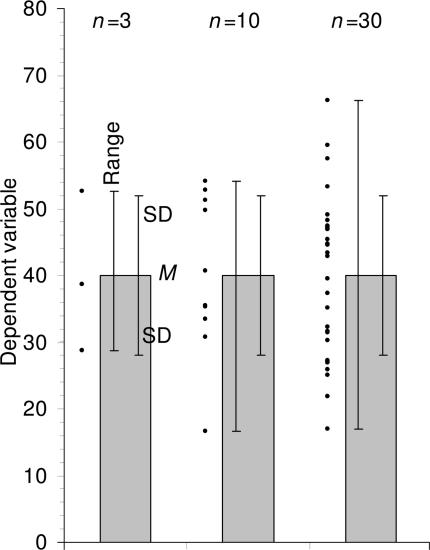
Range and standard deviation (SD) are used for descriptive error bars because they show how the data are spread (Fig. 1). Range error bars encompass the lowest and highest values. SD is calculated by the formula

where X refers to the individual data points, M is the mean, and Σ (sigma) means add to find the sum, for all the n data points. SD is, roughly, the average or typical difference between the data points and their mean, M. About two thirds of the data points will lie within the region of mean ± 1 SD, and ∼95% of the data points will be within 2 SD of the mean.

It is highly desirable to use larger n, to achieve narrower inferential error bars and more precise estimates of true population values.

Figure 1.

Descriptive error bars. Means with error bars for three cases: n = 3, n = 10, and n = 30. The small black dots are data points, and the column denotes the data mean M. The bars on the left of each column show range, and the bars on the right show standard deviation (SD). M and SD are the same for every case, but notice how much the range increases with n. Note also that although the range error bars encompass all of the experimental results, they do not necessarily cover all the results that could possibly occur. SD error bars include about two thirds of the sample, and 2 x SD error bars would encompass roughly 95% of the sample.

Descriptive error bars can also be used to see whether a single result fits within the normal range. For example, if you wished to see if a red blood cell count was normal, you could see whether it was within 2 SD of the mean of the population as a whole. Less than 5% of all red blood cell counts are more than 2 SD from the mean, so if the count in question is more than 2 SD from the mean, you might consider it to be abnormal.

As you increase the size of your sample, or repeat the experiment more times, the mean of your results (M) will tend to get closer and closer to the true mean, or the mean of the whole population, μ. We can use M as our best estimate of the unknown μ. Similarly, as you repeat an experiment more and more times, the SD of your results will tend to more and more closely approximate the true standard deviation (σ) that you would get if the experiment was performed an infinite number of times, or on the whole population. However, the SD of the experimental results will approximate to σ, whether n is large or small. Like M, SD does not change systematically as n changes, and we can use SD as our best estimate of the unknown σ, whatever the value of n.

Inferential error bars.

In experimental biology it is more common to be interested in comparing samples from two groups, to see if they are different. For example, you might be comparing wild-type mice with mutant mice, or drug with placebo, or experimental results with controls. To make inferences from the data (i.e., to make a judgment whether the groups are significantly different, or whether the differences might just be due to random fluctuation or chance), a different type of error bar can be used. These are standard error (SE) bars and confidence intervals (CIs). The mean of the data, M, with SE or CI error bars, gives an indication of the region where you can expect the mean of the whole possible set of results, or the whole population, μ, to lie (Fig. 2). The interval defines the values that are most plausible for μ.

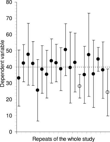
Figure 2.

Confidence intervals. Means and 95% CIs for 20 independent sets of results, each of size n = 10, from a population with mean μ = 40 (marked by the dotted line). In the long run we expect 95% of such CIs to capture μ; here 18 do so (large black dots) and 2 do not (open circles). Successive CIs vary considerably, not only in position relative to μ, but also in length. The variation from CI to CI would be less for larger sets of results, for example n = 30 or more, but variation in position and in CI length would be even greater for smaller samples, for example n = 3.

Because error bars can be descriptive or inferential, and could be any of the bars listed in Table I or even something else, they are meaningless, or misleading, if the figure legend does not state what kind they are. This leads to the first rule. Rule 1: when showing error bars, always describe in the figure legends what they are.

Statistical significance tests and P values

If you carry out a statistical significance test, the result is a P value, where P is the probability that, if there really is no difference, you would get, by chance, a difference as large as the one you observed, or even larger. Other things (e.g., sample size, variation) being equal, a larger difference in results gives a lower P value, which makes you suspect there is a true difference. By convention, if P < 0.05 you say the result is statistically significant, and if P < 0.01 you say the result is highly significant and you can be more confident you have found a true effect. As always with statistical inference, you may be wrong! Perhaps there really is no effect, and you had the bad luck to get one of the 5% (if P < 0.05) or 1% (if P < 0.01) of sets of results that suggests a difference where there is none. Of course, even if results are statistically highly significant, it does not mean they are necessarily biologically important. It is also essential to note that if P > 0.05, and you therefore cannot conclude there is a statistically significant effect, you may not conclude that the effect is zero. There may be a real effect, but it is small, or you may not have repeated your experiment often enough to reveal it. It is a common and serious error to conclude “no effect exists” just because P is greater than 0.05. If you measured the heights of three male and three female Biddelonian basketball players, and did not see a significant difference, you could not conclude that sex has no relationship with height, as a larger sample size might reveal one. A big advantage of inferential error bars is that their length gives a graphic signal of how much uncertainty there is in the data: The true value of the mean μ we are estimating could plausibly be anywhere in the 95% CI. Wide inferential bars indicate large error; short inferential bars indicate high precision.

Replicates or independent samples—what is n?

Science typically copes with the wide variation that occurs in nature by measuring a number (n) of independently sampled individuals, independently conducted experiments, or independent observations.

Rule 2: the value of n (i.e., the sample size, or the number of independently performed experiments) must be stated in the figure legend.

It is essential that n (the number of independent results) is carefully distinguished from the number of replicates, which refers to repetition of measurement on one individual in a single condition, or multiple measurements of the same or identical samples. Consider trying to determine whether deletion of a gene in mice affects tail length. We could choose one mutant mouse and one wild type, and perform 20 replicate measurements of each of their tails. We could calculate the means, SDs, and SEs of the replicate measurements, but these would not permit us to answer the central question of whether gene deletion affects tail length, because n would equal 1 for each genotype, no matter how often each tail was measured. To address the question successfully we must distinguish the possible effect of gene deletion from natural animal-to-animal variation, and to do this we need to measure the tail lengths of a number of mice, including several mutants and several wild types, with n > 1 for each type.

Similarly, a number of replicate cell cultures can be made by pipetting the same volume of cells from the same stock culture into adjacent wells of a tissue culture plate, and subsequently treating them identically. Although it would be possible to assay the plate and determine the means and errors of the replicate wells, the errors would reflect the accuracy of pipetting, not the reproduciblity of the differences between the experimental cells and the control cells. For replicates, n = 1, and it is therefore inappropriate to show error bars or statistics.

If an experiment involves triplicate cultures, and is repeated four independent times, then n = 4, not 3 or 12. The variation within each set of triplicates is related to the fidelity with which the replicates were created, and is irrelevant to the hypothesis being tested.

To identify the appropriate value for n, think of what entire population is being sampled, or what the entire set of experiments would be if all possible ones of that type were performed. Conclusions can be drawn only about that population, so make sure it is appropriate to the question the research is intended to answer.

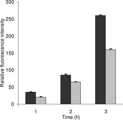
In the example of replicate cultures from the one stock of cells, the population being sampled is the stock cell culture. For n to be greater than 1, the experiment would have to be performed using separate stock cultures, or separate cell clones of the same type. Again, consider the population you wish to make inferences about—it is unlikely to be just a single stock culture. Whenever you see a figure with very small error bars (such as Fig. 3), you should ask yourself whether the very small variation implied by the error bars is due to analysis of replicates rather than independent samples. If so, the bars are useless for making the inference you are considering.

Figure 3.

Inappropriate use of error bars. Enzyme activity for MEFs showing mean + SD from duplicate samples from one of three representative experiments. Values for wild-type vs. −/− MEFs were significant for enzyme activity at the 3-h timepoint (P < 0.0005). This figure and its legend are typical, but illustrate inappropriate and misleading use of statistics because n = 1. The very low variation of the duplicate samples implies consistency of pipetting, but says nothing about whether the differences between the wild-type and −/− MEFs are reproducible. In this case, the means and errors of the three experiments should have been shown.

Sometimes a figure shows only the data for a representative experiment, implying that several other similar experiments were also conducted. If a representative experiment is shown, then n = 1, and no error bars or P values should be shown. Instead, the means and errors of all the independent experiments should be given, where n is the number of experiments performed.

Rule 3: error bars and statistics should only be shown for independently repeated experiments, and never for replicates. If a “representative” experiment is shown, it should not have error bars or P values, because in such an experiment, n = 1 (Fig. 3 shows what not to do).

What type of error bar should be used?

Rule 4: because experimental biologists are usually trying to compare experimental results with controls, it is usually appropriate to show inferential error bars, such as SE or CI, rather than SD. However, if n is very small (for example n = 3), rather than showing error bars and statistics, it is better to simply plot the individual data points.

What is the difference between SE bars and CIs?

Standard error (SE).

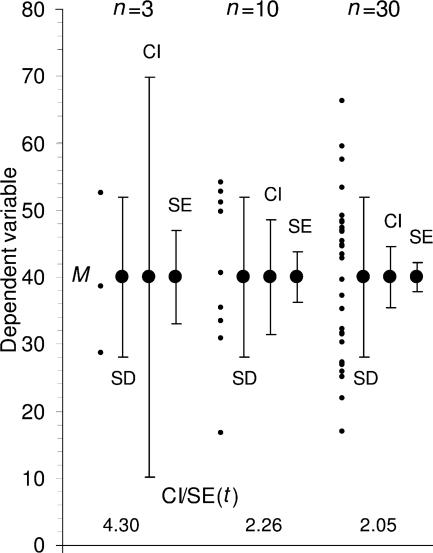
Suppose three experiments gave measurements of 28.7, 38.7, and 52.6, which are the data points in the n = 3 case at the left in Fig. 1. The mean of the data is M = 40.0, and the SD = 12.0, which is the length of each arm of the SD bars. M (in this case 40.0) is the best estimate of the true mean μ that we would like to know. But how accurate an estimate is it? This can be shown by inferential error bars such as standard error (SE, sometimes referred to as the standard error of the mean, SEM) or a confidence interval (CI). SE is defined as SE = SD/√n. In Fig. 4, the large dots mark the means of the same three samples as in Fig. 1. For the n = 3 case, SE = 12.0/√3 = 6.93, and this is the length of each arm of the SE bars shown.

Figure 4.

Inferential error bars. Means with SE and 95% CI error bars for three cases, ranging in size from n = 3 to n = 30, with descriptive SD bars shown for comparison. The small black dots are data points, and the large dots indicate the data mean M. For each case the error bars on the left show SD, those in the middle show 95% CI, and those on the right show SE. Note that SD does not change, whereas the SE bars and CI both decrease as n gets larger. The ratio of CI to SE is the t statistic for that n, and changes with n. Values of t are shown at the bottom. For each case, we can be 95% confident that the 95% CI includes μ, the true mean. The likelihood that the SE bars capture μ varies depending on n, and is lower for n = 3 (for such low values of n, it is better to simply plot the data points rather than showing error bars, as we have done here for illustrative purposes).

The SE varies inversely with the square root of n, so the more often an experiment is repeated, or the more samples are measured, the smaller the SE becomes (Fig. 4). This allows more and more accurate estimates of the true mean, μ, by the mean of the experimental results, M.

We illustrate and give rules for n = 3 not because we recommend using such a small n, but because researchers currently often use such small n values and it is necessary to be able to interpret their papers. It is highly desirable to use larger n, to achieve narrower inferential error bars and more precise estimates of true population values.

Confidence interval (CI).

Fig. 2 illustrates what happens if, hypothetically, 20 different labs performed the same experiments, with n = 10 in each case. The 95% CI error bars are approximately M ± 2xSE, and they vary in position because of course M varies from lab to lab, and they also vary in width because SE varies. Such error bars capture the true mean μ on ∼95% of occasions—in Fig. 2, the results from 18 out of the 20 labs happen to include μ. The trouble is in real life we don't know μ, and we never know if our error bar interval is in the 95% majority and includes μ, or by bad luck is one of the 5% of cases that just misses μ.

The error bars in Fig. 2 are only approximately M ± 2xSE. They are in fact 95% CIs, which are designed by statisticians so in the long run exactly 95% will capture μ. To achieve this, the interval needs to be M ± t _(n–1) ×SE, where t _(n–1) is a critical value from tables of the t statistic. This critical value varies with n. For n = 10 or more it is ∼2, but for small n it increases, and for n = 3 it is ∼4. Therefore M ± 2xSE intervals are quite good approximations to 95% CIs when n is 10 or more, but not for small n. CIs can be thought of as SE bars that have been adjusted by a factor (t) so they can be interpreted the same way, regardless of n.

This relation means you can easily swap in your mind's eye between SE bars and 95% CIs. If a figure shows SE bars you can mentally double them in width, to get approximate 95% CIs, as long as n is 10 or more. However, if n = 3, you need to multiply the SE bars by 4.

Rule 5: 95% CIs capture μ on 95% of occasions, so you can be 95% confident your interval includes μ. SE bars can be doubled in width to get the approximate 95% CI, provided n is 10 or more. If n = 3, SE bars must be multiplied by 4 to get the approximate 95% CI.

Determining CIs requires slightly more calculating by the authors of a paper, but for people reading it, CIs make things easier to understand, as they mean the same thing regardless of n. For this reason, in medicine, CIs have been recommended for more than 20 years, and are required by many journals (7).

Fig. 4 illustrates the relation between SD, SE, and 95% CI. The data points are shown as dots to emphasize the different values of n (from 3 to 30). The leftmost error bars show SD, the same in each case. The middle error bars show 95% CIs, and the bars on the right show SE bars—both these types of bars vary greatly with n, and are especially wide for small n. The ratio of CI/SE bar width is t _(n–1); the values are shown at the bottom of the figure. Note also that, whatever error bars are shown, it can be helpful to the reader to show the individual data points, especially for small n, as in Figs. 1 and 4, and rule 4.

Using inferential intervals to compare groups

When comparing two sets of results, e.g., from n knock-out mice and n wild-type mice, you can compare the SE bars or the 95% CIs on the two means (6). The smaller the overlap of bars, or the larger the gap between bars, the smaller the P value and the stronger the evidence for a true difference. As well as noting whether the figure shows SE bars or 95% CIs, it is vital to note n, because the rules giving approximate P are different for n = 3 and for n ≥ 10.

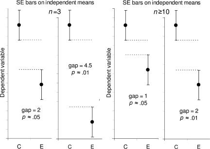
Fig. 5 illustrates the rules for SE bars. The panels on the right show what is needed when n ≥ 10: a gap equal to SE indicates P ≈ 0.05 and a gap of 2SE indicates P ≈ 0.01. To assess the gap, use the average SE for the two groups, meaning the average of one arm of the group C bars and one arm of the E bars. However, if n = 3 (the number beloved of joke tellers, Snark hunters (8), and experimental biologists), the P value has to be estimated differently. In this case, P ≈ 0.05 if double the SE bars just touch, meaning a gap of 2 SE.

Figure 5.

Estimating statistical significance using the overlap rule for SE bars. Here, SE bars are shown on two separate means, for control results C and experimental results E, when n is 3 (left) or n is 10 or more (right). “Gap” refers to the number of error bar arms that would fit between the bottom of the error bars on the controls and the top of the bars on the experimental results; i.e., a gap of 2 means the distance between the C and E error bars is equal to twice the average of the SEs for the two samples. When n = 3, and double the length of the SE error bars just touch (i.e., the gap is 2 SEs), P is ∼0.05 (we don't recommend using error bars where n = 3 or some other very small value, but we include rules to help the reader interpret such figures, which are common in experimental biology).

Rule 6: when n = 3, and double the SE bars don't overlap, P < 0.05, and if double the SE bars just touch, P is close to 0.05 (Fig. 5, leftmost panel). If n is 10 or more, a gap of SE indicates P ≈ 0.05 and a gap of 2 SE indicates P ≈ 0.01 (Fig. 5, right panels).

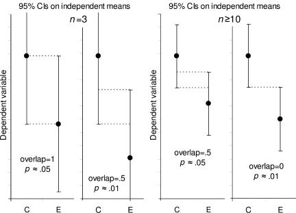
Rule 5 states how SE bars relate to 95% CIs. Combining that relation with rule 6 for SE bars gives the rules for 95% CIs, which are illustrated in Fig. 6. When n ≥ 10 (right panels), overlap of half of one arm indicates P ≈ 0.05, and just touching means P ≈ 0.01. To assess overlap, use the average of one arm of the group C interval and one arm of the E interval. If n = 3 (left panels), P ≈ 0.05 when two arms entirely overlap so each mean is about lined up with the end of the other CI. If the overlap is 0.5, P ≈ 0.01.

Figure 6.

Estimating statistical significance using the overlap rule for 95% CI bars. Here, 95% CI bars are shown on two separate means, for control results C and experimental results E, when n is 3 (left) or n is 10 or more (right). “Overlap” refers to the fraction of the average CI error bar arm, i.e., the average of the control (C) and experimental (E) arms. When n ≥ 10, if CI error bars overlap by half the average arm length, P ≈ 0.05. If the tips of the error bars just touch, P ≈ 0.01.

Rule 7: with 95% CIs and n = 3, overlap of one full arm indicates P ≈ 0.05, and overlap of half an arm indicates P ≈ 0.01 (Fig. 6, left panels).

Repeated measurements of the same group

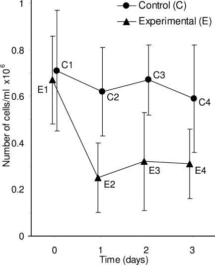
The rules illustrated in Figs. 5 and 6 apply when the means are independent. If two measurements are correlated, as for example with tests at different times on the same group of animals, or kinetic measurements of the same cultures or reactions, the CIs (or SEs) do not give the information needed to assess the significance of the differences between means of the same group at different times because they are not sensitive to correlations within the group. Consider the example in Fig. 7, in which groups of independent experimental and control cell cultures are each measured at four times. Error bars can only be used to compare the experimental to control groups at any one time point. Whether the error bars are 95% CIs or SE bars, they can only be used to assess between group differences (e.g., E1 vs. C1, E3 vs. C3), and may not be used to assess within group differences, such as E1 vs. E2.

Figure 7.

Inferences between and within groups. Means and SE bars are shown for an experiment where the number of cells in three independent clonal experimental cell cultures (E) and three independent clonal control cell cultures (C) was measured over time. Error bars can be used to assess differences between groups at the same time point, for example by using an overlap rule to estimate P for E1 vs. C1, or E3 vs. C3; but the error bars shown here cannot be used to assess within group comparisons, for example the change from E1 to E2.

Assessing a within group difference, for example E1 vs. E2, requires an analysis that takes account of the within group correlation, for example a Wilcoxon or paired t analysis. A graphical approach would require finding the E1 vs. E2 difference for each culture (or animal) in the group, then graphing the single mean of those differences, with error bars that are the SE or 95% CI calculated from those differences. If that 95% CI does not include 0, there is a statistically significant difference (P < 0.05) between E1 and E2.

Rule 8: in the case of repeated measurements on the same group (e.g., of animals, individuals, cultures, or reactions), CIs or SE bars are irrelevant to comparisons within the same group (Fig. 7).

Conclusion

Error bars can be valuable for understanding results in a journal article and deciding whether the authors' conclusions are justified by the data. However, there are pitfalls. When first seeing a figure with error bars, ask yourself, “What is n? Are they independent experiments, or just replicates?” and, “What kind of error bars are they?” If the figure legend gives you satisfactory answers to these questions, you can interpret the data, but remember that error bars and other statistics can only be a guide: you also need to use your biological understanding to appreciate the meaning of the numbers shown in any figure.

References

- 1.Belia, S., F. Fidler, J. Williams, and G. Cumming. 2005. Researchers misunderstand confidence intervals and standard error bars. Psychol. Methods. 10:389–396. [DOI] [PubMed] [Google Scholar]
- 2.Cumming, G., J. Williams, and F. Fidler. 2004. Replication, and researchers' understanding of confidence intervals and standard error bars. Understanding Statistics. 3:299–311. [Google Scholar]
- 3.Vaux, D.L. 2004. Error message. Nature. 428:799. [DOI] [PubMed] [Google Scholar]
- 4.Cumming, G., F. Fidler, M. Leonard, P. Kalinowski, A. Christiansen, A. Kleinig, J. Lo, N. McMenamin, and S. Wilson. 2007. Statistical reform in psychology: Is anything changing? Psychol. Sci. In press. [DOI] [PubMed]
- 5.Schenker, N., and J.F. Gentleman. 2001. On judging the significance of differences by examining the overlap between confidence intervals. Am. Stat. 55:182–186. [Google Scholar]
- 6.Cumming, G., and S. Finch. 2005. Inference by eye: Confidence intervals, and how to read pictures of data. Am. Psychol. 60:170–180. [DOI] [PubMed] [Google Scholar]
- 7.International Committee of Medical Journal Editors. 1997. Uniform requirements for manuscripts submitted to biomedical journals. Ann. Intern. Med. 126:36–47. [DOI] [PubMed] [Google Scholar]
- 8.Carroll, L. 1876. The hunting of the snark An agony in 8 fits. Macmillan, London. 83 pp.