Abstract
Rationale and Objectives
We have previously described a probabilistic model for the multiple-reader, multiple-case paradigm for ROC analysis. When the figure of merit is the Wilcoxon statistic, this model returns a seven-term expansion for the variance of this statistic as a function of the numbers of cases and readers. This probabilistic model also provides expressions for the coefficients in the seven-term expansion in terms of expectations over the internal noise, readers, and cases. Finally, this probabilistic model sets bounds on both the overall variance of the Wilcoxon statistic as well as the individual coefficients.
Materials and Methods
In this paper we will first validate the probabilistic model by comparing variances determined by direct computation of the expansion coefficients to empirical estimates of the variance using independent sampling. Validation of the probabilistic model will enable us to use the direct estimates of the expansion coefficients as a gold-standard to compare other coefficient-estimation techniques. Next, we develop a coefficient-estimation technique that employs bootstrapping to estimate the Wilcoxon statistic variance for different numbers of readers and cases. We then employ constrained, least-squares fitting techniques to estimate the expansion coefficients. The constraints used in this fitting are derived directly from the probabilistic model.
Results and Discussion
Using two different simulation studies, we show that the novel (and practical) bootstrapping/fitting technique returns estimates of the coefficients that are consistent with the gold standard. The results presented also serve to validate the seven-term expansion for the variance of the Wilcoxon statistic.
Keywords: ROC analysis, multiple reader multiple case, Wilcoxon statistic
1. INTRODUCTION
Receiver operating characteristic (ROC) analysis is the standard method used to assess imaging technologies for radiology, as well as other diagnostic procedures. ROC studies are typically time consuming and expensive. Therefore, considerable effort has been devoted to analyzing sources of variability and designing experiments to maximize statistical power. A large part of this effort involves identifying and estimating sources of variability in the area under the ROC curve (AUC) or other figures of merit associated with the ROC curve. The major sources of variability in ROC studies are caused by the finite number of readers, the finite number of cases, and the reader internal noise.
In the multiple-reader, multiple-case (MRMC) paradigm, each member of a sample of readers reads all of the cases in a sample of cases. Each reader produces a rating (or test statistic) for each case which represents her or his confidence that an abnormality, such as a tumor, is present. The end result is an array of test statistics which is then used to compute a figure of merit for the imaging system being tested. In MRMC analysis, we are not only interested in the value of the chosen figure of merit, we are also interested in the variance of this number as a function of the numbers of readers and cases. This information aids in the design of the ROC studies and can help ensure that the results are statistically meaningful.
Standard methods for MRMC analysis have used linear models and analysis of variance (ANOVA) techniques to determine the variance of the figure of merit as a function of numbers of readers and cases [1, 2]. Bootstrapping techniques have also been employed using the same linear model [3]. With the linear model, one assumes that the figure of merit can be expanded as a sum of independent random variables; one that depends on the reader sample, one that depends on the case sample, one that depends on the reader-case interaction, and a final variable that describes internal reader noise. The variance of the figure of merit then becomes a sum of the variances of the individual terms. The validity of the results obtained using this model depends, of course, on the validity of the initial linear model. Even if the terms in the linear model are not independent, the expression for the variance can be considered a first-order expansion for the variance of the figure of merit.
The probabilistic approach, as described in Clarkson et al. [4], builds on the work of Hoeffding [5] and Lehmann [6] and is based on a probability model for the generation of reader test statistics. This probability model accounts for random cases, random readers, and internal noise. The readers are chosen independently from a population of readers, cases are chosen independently from a population of cases, and the reader sample is independent of the case sample. A reader’s test statistic is a random variable whose distribution depends on the interaction of the reader with a case as well as the internal noise of the reader. When this probabilistic model is applied to the Wilcoxon statistic [7, 8], the result is an exact, seven-term expansion for the variance of this statistic in terms of the numbers of readers and cases.
In this paper, we both validate the probabilistic model and present a method for computing the coefficients in the seven-term expansion. To validate the probabilistic model, we directly compute the expansion coefficients from expectations derived from the probabilistic model. The computation of these expectations combines analytical formulas with Monte-Carlo techniques to compute the relevant expectations. The variance derived from the direct computation of the expansion coefficients can then be compared to empirical estimates of variance computed using independent sampling. Once the probabilistic model has been validated, these direct estimates of the model coefficients can be used a gold standard to compare our new estimation technique. Our estimation technique uses bootstrapping to estimate the variance of the Wilcoxon statistic at many choices of numbers of readers and cases. The resulting data are then fit to the seven-term expansion using constrained least-squares fitting techniques. The bounds on the coefficients derived from the probabilistic model are used as constraints for the fitting. This method, unlike the direct computation of the coefficients and the independent sampling technique, requires only a single reader and case sample.
Two separate simulations are used to validate the model and evaluate the bootstrap-estimation technique. For the first simulation (or data model), we employ a very simplistic representation for the cases and readers. A single case is represented by a Gaussian-distributed random variable, the mean of which depends on the truth state. A reader is represented by a pair of numbers each sampled from a uniform distribution centered up 1.0. The reader-case interaction is described by a simple multiplication of one reader random variables with a case random variable. The truth state of the case determines which reader random variable is employed. After adding a Gaussian random variable to this product to simulate internal noise, we have the test statistic for the given reader and case. This model, while simplistic, does account for reader proficiency, reader-case interaction, and internal noise. One advantage of this model is that expectations over internal noise and cases can be computed analytically. All that is left is to perform the average over readers to compute the expectations needed for the direct computation of the expansion coefficients.
For the second, more realistic, simulation, we employ a lumpy background model for the signal-absent images and add in a known signal for the signal-present images. Detector noise is modeled as being Poisson distributed. A reader is described by an image called a template that has the same dimensions as the case images. The templates have a single, random width parameter that represents the reader variability. A reader reads an image by taking the inner product of the template with the image and adding Gaussian noise to account for internal noise. For this simulation, expectations over internal noise can still be performed analytically but Monte-Carlo methods must be used for averages over readers and cases.
By comparing the results from the direct computation to independent sampling results, we will validate the probabilistic model and the seven-term expansion. By comparing the results of the bootstrap method to the other two, we will demonstrate the usefulness of the bootstrap method for estimating the seven coefficients.
2. PROBABILISTIC MODEL
We will briefly review the probabilistic MRMC model. For a detailed derivation of this model, consult Clarkson et al. [4] and Barrett et al. [9]. The probabilistic models begins by considering random cases, readers, and test statistics. A case from the signal-absent ensemble is represented by a random vector g0 (bold-face type denotes vectors), while a case from a single-present ensemble is represented by the random vector g1. These random vectors have corresponding distribution given by pr(g0) and pr(g1). A case sample is composed of N0 independent samples from pr(g0) and N1 independent samples from pr(g1).
A reader is represented by a random vector γ with distribution pr(γ). This reader vector may represent a mathematical representation of a reader or simply an identifying string, e.g., reader 58 out of 1000 or “Mary.” A reader sample consists of Nr independent samples from pr(γ).
Given a reader γ and a case ga (a is 0 or 1), the test statistic ta is a random variable with a conditional distribution give by pr(ta|γ, ga). This conditional distribution encompasses the reader-case interaction and describes the internal noise for reader γ. Given a case sample and reader sample, the entries in the test statistic matrix are independent samples from the corresponding conditional distributions, one for each reader-case pair. For example, the entry for the reader γr (i.e., the rth reader in the reader sample), and signal-absent case g0i (i.e., the ith signal-absent case in the case sample) is t0ri and this is a sample from the distribution pr(t|γr, g0i). Similarly, the entry for the reader γr and signal-present case g0j is t1rj and this is a sample from the distribution pr(t|γr, g1j).
Using this notation, the Wilcoxon figure of merit is given by
| (1) |
where s(·) is the step function. The Wilcoxon statistic  is an estimate of the area under the ROC curve (or AUC) averaged over all readers. We have previously shown [4] that the variance of  can be written exactly as the seven-term expansion:
| (2) |
Here the αn are coefficients to be determined.
Not only does the probabilistic model return an exact, seven-term expansion, it also gives analytic expressions for each of the αn terms. These expressions can be used in simulation studies to determine the correct values of the αn for comparison with estimation methods. It is useful to first define,
| (3) |
| (4) |
For ease of notation, we drop the i, j, and r subscripts to arrive at s̄(γ, g0, g1) and s̿(g0, g1). The term s̄(γ, g0, g1) represents the average step-function response of reader γ reading the pair of cases g0 and g1. This is analogous to a two-alternative forced choice (2AFC) experiment where a particular reader is determining which of a pair images has the abnormality. It is well known that the fraction of correct decisions that the reader makes is the AUC for that reader on that set of images. Thus, s̄(γ, g0, g1) can be thought of as the AUC of a reader reading a pair of images when the reader has perfect memory loss after each reading; it is an average over reader-internal noise only. The term s̿(g0, g1) is the average of s̄(γ, g0, g1) over all readers γ. Again, using the 2AFC analogy, s̿(g0, g1) can be thought of as the average AUC of all readers reading the pair of images g0 and g1.
With both s̄(·) and s̿(·) defined, we can now write the first four αn terms as
| (5) |
| (6) |
| (7) |
| (8) |
The remaining terms, while not as simple as α1 through α4, can also be written in terms of expectations of s(·),
| (9) |
| (10) |
| (11) |
Finally, utilizing the fact that variances must be positive and variances of quantities bounded between zero and one must not exceed , we can derive bounds on each of the αn. Namely,
| (12) |
| (13) |
| (14) |
| (15) |
| (16) |
| (17) |
| (18) |
| (19) |
For a detailed derivation of these bounds, refer to Clarkson et al. [4].
3. METHODS
To both validate the probabilistic model and test methods for estimating the coefficients, we examined two data models. We first describe the two data models and then the coefficient-estimation techniques.
3.1 Data Model 1
The first data model was designed to include reader variability, case variability, reader-case interactions, and internal noise yet be simple enough to allow analytical computations of expectations (Eqns. 5–11). To achieve this simplicity, cases are represented by a single random variable g0 or g1 distributed as (0, 1) and (μ, 1), respectively. Here, μ is an adjustable model parameter that represents the signal strength. A reader is represented by a pair of random variables c0 and c1 both independently distributed as (1 − Δ, 1 + Δ). The parameter Δ is an adjustable parameter relating to the reader variability. The test statistics are generated by
| (20) |
| (21) |
where η0 and η1 are both independently and represent the reader internal noise. The term σt controls the amount of internal noise. It should be noted that the terms c0 and c1 are random across readers but are fixed for a given reader.
The reason for using a pair of numbers for the readers is to account for varying reader skill. The reader-case interaction arises because the reader parameters are multiplied by the case variables. Note that for a fixed reader, t0 and t1 are Gaussian random variables. This fact means that averages over internal noise and cases conditioned on readers can be computed analytically. For our simulations, μ = 1, Δ = 0.95, and σt = 0.3.
3.2 Data Model 2
For the second, more realistic, data model we employed simulated images and linear readers. The cases are simulated images that are generated by a two-dimensional “lumpy” image model with Poisson noise added. The mean of the mth pixel in the lumpy image model is given by,
| (22) |
where rm is the two-dimensional coordinate vector for the mth pixel, L is the number of lumps, l(·) is the lump function (typically Gaussian), and cl is the center of the lth lump. Here, L is a Poisson-distributed random variable with mean L̄, and the cl are random locations with a uniform distribution across the image. For signal-present cases, a small (relative to the lump size) Gaussian signal is added to the mean image at its center or the (0,0) location.
For this model, we chose an image size of 64 pixels by 64 pixels, i.e., g is a 642-dimensional vector. The mean number of lumps L̄ was 25. This relatively small number ensures that the statistics governing g0 and g1 are not Gaussian. The lump function was a Gaussian with a standard deviation of 5 pixels and an amplitude of 20 units. The signal was a Gaussian function with a standard deviation of 3 pixels and an amplitude of 35 units.
A reader was simulated by also generating an image called a template. The mth pixel in this template is given by
| (23) |
Here σ is the width of the template. Note that this Gaussian template is always centered on the signal location. The width of the template σ is a random variable uniformly distributed between 1 and 10 pixels. Templates with different σ parameters will perform differently. Thus, the random σ parameter accounts for varying reader skill.
Finally, the test statistics are generated by taking the inner product of a reader template with an image and adding noise to simulate internal noise. That is,
| (24) |
| (25) |
Note that the random variables η0 and η1 are independent Gaussians with standard deviations of 5. Again, this model accounts for case variability, reader variability and internal noise. However, unlike the previous model, we will not be able to perform the case-averages analytically because of the non-Gaussian, high-dimensional distributions associated with g0 and g1.
3.3 Variance Estimation Techniques
3.3.1 Direct Computation
An advantage of the probabilistic model is that it returns analytic expressions for the αn coefficients. We have numerically evaluated Eqns. 5–11 to arrive at estimates for the αn. For data model 1, any conditional expectation where the reader γ is fixed, such as s̄(γ, g0, g1), can be computed exactly in terms of error functions. Other expectations must be computed via Monte-Carlo integration. For data model 2, s̄(γ, g0, g1) can still be computed exactly but all other expectations must be computed by Monte-Carlo integration. When Monte-Carlo integration was required, we employed 10,000 samples to estimate the expectations. The αn returned by this direct computation will serve as our gold standard which will be used to assess the other techniques.
It should be noted that direct computation of the αn is not possible using a single dataset because replication over internal noise must be performed. Thus, this method is useful only for mathematical observers, validating the probabilistic model or validating new estimation techniques.
3.3.2 Independent sampling
To validate the seven-term expansion, we employed independent sampling to estimate the variance of the Wilcoxon statistic at varying numbers of readers and cases. For a given number of readers and cases, we generated 10,000 independent reader and case samples. We then generate the matrix of test statistics (with internal noise) by having each reader read each case in the corresponding sample (including internal noise). From these 10,000 test-statistic matrices, we compute 10,000 AUCs and estimate the AUC variance. Thus, we can estimate the AUC variance for any numbers or readers and cases (i.e., any Nr, N0, and N1) and compare these results to the results returned by direct computation.
3.3.3 Bootstrap sampling
With real data, one cannot use either of the first two techniques since independent samples are not readily available and the distributions of the random variables are not known. Typically, a single test-statistic matrix is all that we have to work with. With just a single sample, however, we can exploit bootstrapping techniques to estimate variances. In this procedure, reader and case samples are drawn by bootstrapping. We then extract all of the test statistics for the selected readers and cases. The AUC for this bootstrap sample can be readily computed using Eqn. 1. A total of 1000 test-statistic matrices are generated by bootstrapping for different choices of Nr, N0, and N1. By evaluating the AUC variance for different combinations of numbers of cases and readers, we can generate data which can be used to fit the αn parameters in the seven-term expansion. This fitting process is not only linear (see Eqn. 2) but also constrained (Eqns. 12–19). Thus, constrained linear least-squares fitting is used to determine the αn. These results can be compared with the direction computation technique to assess the usefulness of this procedure.
4. RESULTS
4.1 Data Model 1
Due to the simplicity of the first data model, many of the expectations in Eqns. 5–11 can be computed analytically. Only expectations over readers must be computed using Monte-Carlo methods. Thus, direct and accurate computation of the αn can be performed. These αn are used as the gold standard with which to compare the independent sampling and the bootstrap techniques for estimating the αn. We employed 10,000 samples to compute expectations over readers.
Figure 1 compares the variance computed using the direct computation of the αn (solid line) to the measured variance of AUC using 10,000 independent reader and case samples with varying Nr, N0 and N1. In Fig. 1a, the Nr is varied from 1 to 50 and the N0 and N1 are both fixed at 100. In Fig. 1b, Nr is fixed at 5 and both N0 and N1 are varied between 10 and 1000. These plots clearly indicate that the seven-term expansion is accurately predicting the variance of the Wilcoxon statistic for varying Nr, N0, and N1.
Fig. 1.
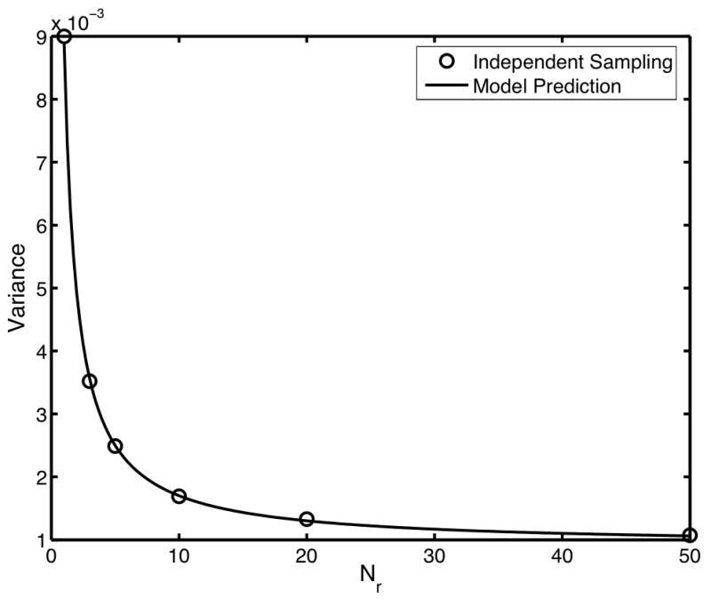
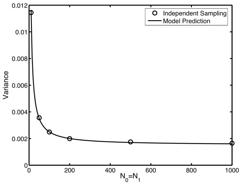
Comparison of the variances predicted using direct computation of the expansion coefficients (solid line) to empirical estimates of the variance computed using independent sampling (circles). In (a), Nr is varied from 1 to 50 with both N0 and N1 fixed at 100. In (b), Nr was fixed at 5 while both N0 and N1 were varied from 10 to 1000. For the independent sampling, 10,000 repetitions were used.
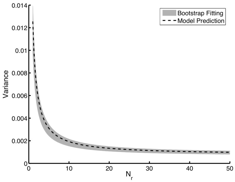
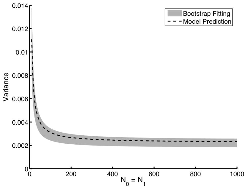
While the results presented in Fig. 1 are important, both the direct computation of the αn and the independent sampling technique are impractical for real data. The direct computation technique requires expectations over internal noise and the independent sampling technique requires an impractical number of readers and cases to be useful. The bootstrapping technique, however, requires only a single sample of readers reading a single case sample to produce a test-statistic matrix. The bootstrap estimates of AUC variance can be used to estimate the individual αn by using constrained, linear, least-squared curve fitting. Using a dataset of 25 readers and 1000 image pairs, we computed the bootstrap estimates of the αn. To perform the fitting, a 3 × 3 × 3 grid of Nr, N0, and N1 was used. These 27 bootstrap estimates of variance were used in the constrained fitting algorithm to determine the αn. This process was repeated 100 times to determine how this algorithm performs on average, i.e., we determine the mean and the standard deviation of each estimated αn parameter. The results of this study are summarized in Fig. 2. The solid line is the gold standard variance computed using the direction computation technique. The gray area represents the mean plus and minus one standard deviation of the bootstrap-estimated αn. Clearly, the bootstrap technique is returning both accurate and precise estimates of αn. We will see with the second data model that small sample sizes can introduce some bias into this estimation technique.
Fig. 2.
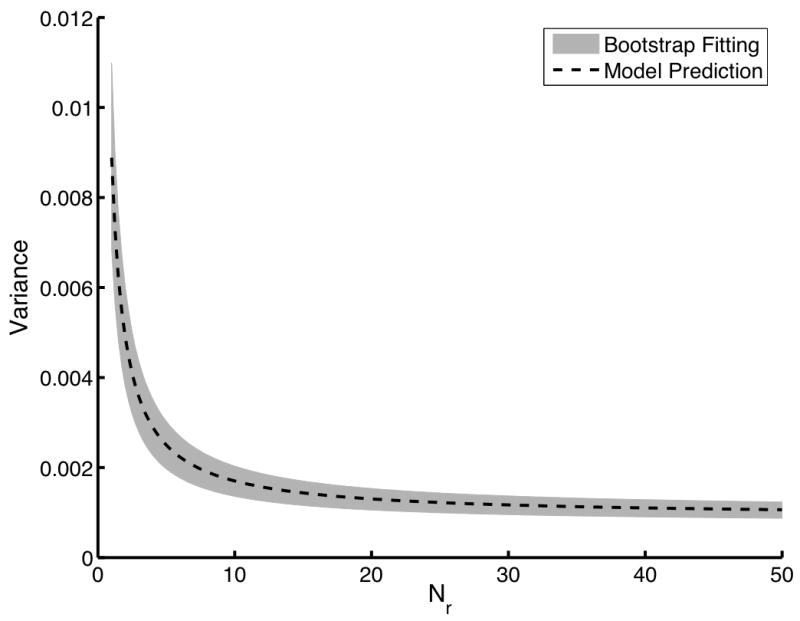
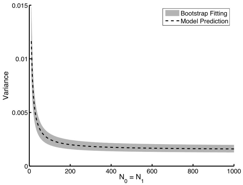

An evaluation of the bootstrap coefficient estimation technique. The dashed line indicates the gold standard computed using the direct computation technique. The gray area represents the mean plus and minus one standard deviation of the variance predicted using the fitted αn. For this study, a single dataset of 25 readers and 1000 image pairs was used to estimate the expansion coefficients. This process was repeated 100 times using 100 different datasets of the same size to determine the mean and the standard deviations of the estimates αn. In (a), Nr is varied from 1 to 50 with both N0 and N1 fixed at 100. In (b), Nr was fixed at 5 while both N0 and N1 were varied from 10 to 1000.
4.2 Data Model 2
We further validated the bootstrap technique using the second data model. This more realistic data model employs images with random backgrounds and Poisson detector noise. A reader was simulated by generating a random template which allows for varying reader skill. Finally, internal noise was simulated as Gaussian. Unlike data model 1, many of the expectations in Eqns. 5–11 cannot be computed analytically. Thus, we employed large samples of readers (10,000) and cases (10,000) to estimate these expectations directly. To ensure that our estimates of αn were accurate, we repeated this experiment multiple times and found that our estimates of αn did not vary through the first three significant digits. Thus, we employed these direct estimates of the αn as the gold standard.
For this second data model, independent sampling is not feasible because of the time needed to generate sufficient numbers of images and readers. The direct computation technique also requires a large sample size. However, only one reader sample and case sample was necessary. Thus, we will present AUC variances determined using only bootstrap estimates of the αn, further validating the bootstrap estimation technique. Figure 3 compares the variance determined using the direct computation of the αn to the mean plus and minus one standard deviation of the variances determined using bootstrap estimates of the αn. As with the first data model, 25 reader and 1000 image pairs were simulated. A 3 × 3 × 3 grid of Nr, N0 and N1 was employed. Again, these 27 bootstrap estimates of variance were used in the constrained fitting algorithm to determine the αn. Clearly, the fitting method is both accurate and precise.
Fig. 3.
An evaluation of the bootstrap coefficient estimation technique using the second data model. The dashed line indicates the gold standard computed using the direct computation technique. The gray area represents the mean plus and minus one standard deviation of the variance predicted using the fitted αn. For this study, a single dataset of 25 readers and 1000 image pairs was used to estimate the expansion coefficients. This process was repeated 100 times using 100 different datasets of the same size to determine the mean and the standard deviations of the estimates αn. In (a), Nr is varied from 1 to 50 with both N0 and N1 fixed at 100. In (b), Nr was fixed at 5 while both N0 and N1 were varied from 10 to 1000.
Figure 4 shows similar results except that only 10 readers were simulated along with 100 pairs of images. Here, we begin to see that the bootstrap estimates of the variances might exhibit some bias when the initial sample is small. However, this bias appears to be small and in the positive direction. Note that Fig. 4 plots the predicted variances well beyond the 10 readers and 100 images pairs used to estimate the αn.
Fig. 4.
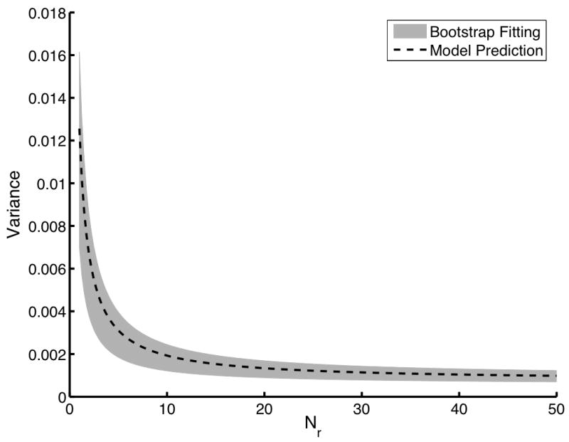
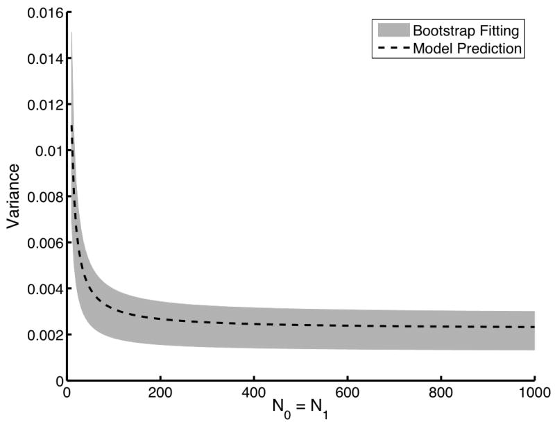
An evaluation of the bootstrap coefficient estimation technique with small datasetes. The dashed line indicates the gold standard computed using the direct computation technique. The gray area represents the mean plus and minus one standard deviation of the variance predicted using the fitted αn. For this study, a single dataset of only 10 readers and 100 image pairs was used to estimate the expansion coefficients. This process was repeated 100 times using 100 different datasets of the same size to determine the mean and the standard deviations of the estimates αn. In (a), Nr is varied from 1 to 50 with both N0 and N1 fixed at 100. In (b), Nr was fixed at 5 while both N0 and N1 were varied from 10 to 1000. Note that while the initial datasets were small, we are accurately predicting variances with much larger Nr, N0, and N1.
5. CONCLUSIONS
Using the probabilistic model we previously showed that variance of the MRMC Wilcoxon statistic can be expressed as a seven-term expansion in terms of Nr, N0, and N1. The probabilistic formulation also results in exact expressions for the seven coefficients in this expansion. With the first data model in this paper, we showed that direct calculation of the coefficients using the probabilistic method gives variances that agree with those computed using independent sampling. This was an important validation to ensure that the no mathematical mistakes were made in the rather complicated derivation of the seven-term expansion. Thus we feel confident in using the direct computation results as gold standards with which to compare other techniques for estimating the αn.
Furthermore, with the first and second data models, we compared the results of our bootstrap/least-squared-fitting technique for estimating the αn to our gold standard. In the first data model, the bootstrap estimation technique worked well in terms of bias and variance. For the second data model, a small bias was introduced when the number of readers is small (i.e., around 5).
In the future, we plan to extend the probabilistic model and our estimation techniques to account for multiple modalities. Preliminary work indicates that an expansion similar to the seven-term expansion for one modality can be derived for two modalities.
Acknowledgments
We thank Drs. Charles Metz, Brandon Gallas and Robert Wagner for their many helpful discussions about this topic. This work was supported by NIH/NCI grant K01 CA87017 and by NIH/NIBIB grants R01 EB002146, R37 EB000803, P41 EB002035.
Footnotes
Publisher's Disclaimer: This is a PDF file of an unedited manuscript that has been accepted for publication. As a service to our customers we are providing this early version of the manuscript. The manuscript will undergo copyediting, typesetting, and review of the resulting proof before it is published in its final citable form. Please note that during the production process errors may be discovered which could affect the content, and all legal disclaimers that apply to the journal pertain.
References
- 1.Dorfman DD, Berbaum KS, Metz CE. Receiver operating characteristic rating analysis. generalization to the population of readers and patients with the jackknife method. Investigative Radiology. 1992;27:723–731. [PubMed] [Google Scholar]
- 2.Roe CA, Metz CE. Variance-component modeling in the analysis of receiver operating characteristic index estimates. Academic Radiology. 1997;4(8):587–600. doi: 10.1016/s1076-6332(97)80210-3. [DOI] [PubMed] [Google Scholar]
- 3.Beiden SV, Wagner RF, Campbell G. Components-of-variance models and multiple-bootstrap experiments: An alternative method for random-effects, receiver operating characteristic analysis. Academic Radiology. 2000;7:342–349. doi: 10.1016/s1076-6332(00)80008-2. [DOI] [PubMed] [Google Scholar]
- 4.Clarkson E, Kupinski MA, Barrett HH. A probabilistic development of the MRMC method. Academic Radiology. 2006;13(10) doi: 10.1016/j.acra.2006.07.016. [DOI] [PMC free article] [PubMed] [Google Scholar]
- 5.Hoeffding W. A class of statistics with asymptotically normal distribution. Annals of Mathematical Statistics. 1948;19:293–325. [Google Scholar]
- 6.Lehmann EL. Consistency and unbiasedness of certain nonparametric tests. Annals of Mathematical Statistics. 1951;22:165–179. [Google Scholar]
- 7.Wilcoxon F. Individual comparison of ranking methods. Biometrics. 1945;1:80–93. [Google Scholar]
- 8.Mann HB, Whitney DR. On a test of whether one of two random variables is stochastically larger than the other. Annals of Mathematical Statistics. 1947;18:50–60. [Google Scholar]
- 9.Barrett HH, Kupinski MA, Clarkson E. Medical Imaging 2005: Image Perception, Observer Performance, and Technology Assessment. 2005. Probabilistic foundations of the MRMC method; pp. 21–31. SPIE. [Google Scholar]


