

Abstract
Matching of corresponding branchpoints between two human airway trees, as well as assigning anatomical names to the segments and branchpoints of the human airway tree, are of significant interest for clinical applications and physiological studies. In the past these tasks were often performed manually due to the lack of automated algorithms that can tolerate false branches and anatomical variability typical for in vivo trees. In this paper we present algorithms that perform both matching of branchpoints and anatomical labeling of in vivo trees without any human intervention and within a short computing time. No hand-pruning of false branches is required. The results from the automated methods show a high degree of accuracy when validated against reference data provided by human experts. 92.9% of the verifiable branchpoint matches found by the computer agree with experts’ results. For anatomical labeling, 97.1% of the automatically assigned segment labels were found to be correct.
Index Terms: Airway tree, branchpoint matching, anatomical labeling
I. INTRODUCTION
The quantitative assessment of intrathoracic airway trees is critically important for the objective evaluation of the bronchial tree structure and function. Functional understanding of pulmonary anatomy, as well as the natural course of respiratory diseases like asthma, emphysema, cystic fibrosis, and many others, is limited by our inability to repeatedly evaluate the same region of the lungs time after time and perform accurate and reliable positionally corresponding measurements. Several approaches to three-dimensional reconstruction of the airway tree have been developed in the past. None of them, however, allows the direct comparison of airway trees across and within subjects.
The first six generations, roughly, of the human airway tree exhibit a relatively similar topology across subjects, and anatomical names exist for 31 segments and 42 sub-segments [1]. Beyond that, the branching structure gets variable and differs very much from subject to subject.
The term branchpoint matching is used for the process of finding corresponding branchpoints between two different scans of the same subject (intra-subject case; e.g., imaged in a longitudinal study or imaged at different lung volumes). This process is based on the similarities of the two input trees and finds matching branchpoints not only for the named segments but also beyond them.
The anatomical labeling algorithm presented here aims to assign 32 anatomical names to their respective segments (the left inferior bronchus was divided into two parts, which accounts for the one additional segmental name compared to the standard nomenclature). Labeling an airway tree does not only simplify the navigation of the tree in applications like virtual bronchoscopy, but also allows matching of branchpoints across subjects (inter-subject case). Another application of anatomical labeling is the identification of lobar and sub-lobar structures, which can, for example, be used for surgical planning.
Both branchpoint matching and anatomical labeling are tedious and error-prone to perform manually; consequently the goal is to automate these tasks. Working with human in-vivo data poses challenges. In-vivo trees deviate from ideal trees because of anatomical variations and because of false-branches introduced by imperfections of the preceding segmentation and skeletonization processes.
Branchpoint matching was mostly done manually in the past [2]. A few attempts of automating the process were undertaken. Pisupati et al. [3], [4] presented a matching algorithm based on dynamic programming that, however, was only applied to very similar pairs of canine trees, and the authors state that they expect the method to fail on human in-vivo scans. Park [5] presented a tree-matching method based on an association graph [6], but his method was applied only to phantom data and it does not tolerate false branches.
Publications about automated anatomical labeling are similarly sparse. Mori et al. [7] presented a knowledge-based labeling algorithm. The proposed algorithm was only applied to incomplete trees (about 30 branches per tree), and the builtin knowledge base did not incorporate anatomical variations. Additionally, the algorithm is sensitive to missing and spurious (false) branches. Kitaoka et al. [8] developed a branchpoint labeling algorithm that uses a mathematical phantom as reference. Labels are assigned by matching the target tree against this phantom. The method can not automatically handle false branches – they have to be pruned manually in a preprocessing step.
A. Input data
In a first step the airway tree is segmented from volumetric computed tomography (CT) images [9], [10] and then skeletonized [11], [12]. Branchpoints are detected in the skeletonization result, and the tree is represented as a directed acyclic graph (DAG) (Figure 1). This DAG is used as input for both the branchpoint matching and the anatomical labeling processes.
Fig. 1.
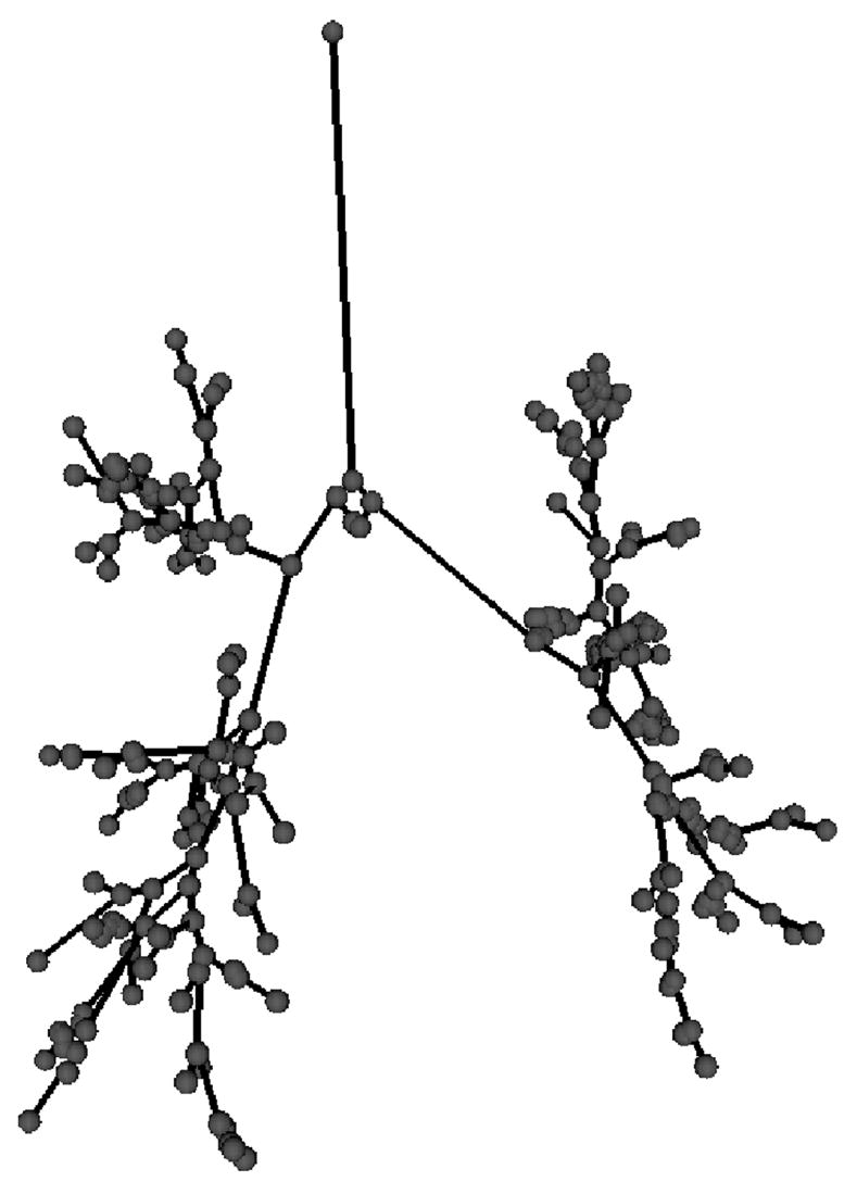
Skeletonized tree represented as a directed acyclic graph (DAG).
II. MATCHING WITH ASSOCIATION GRAPH METHOD
Branchpoint matching and anatomical labeling are both based on matching hierarchical structures (mathematical graphs) using association graphs [6]. Using association graphs for finding graph isomorphisms is a well known technique that has been introduced more than 20 years ago [13].
An association graph is an auxiliary graph structure derived from the two graph structures to be matched. A graph G = (V, E) consists of a set of vertices V and a set of edges E. For two graphs G1 and G2, an association graph Gag = (Vag, Eag) consists of the vertices Vag = V1 × V2. I.e., it contains a vertex for every possible pair of vertices in G1 and G2. Two vertices in Gag are connected with an edge if and only if the corresponding vertices in G1 and G2 stand in the same relationship to each other (e.g., inheritance relationship, topological distance, etc.). The maximum clique in the association graph, i.e., the biggest sub-set of vertices where every pair of vertices is connected by an edge, corresponds to the maximal subtree isomorphism. Each vertex contained in the maximum clique represents a pair of matching vertices in the original graphs. It has been shown [14] that the problem of finding the maximum clique is an NP-complete problem. This paper introduces methods that help keeping the required computing time within very reasonable limits.
III. BRANCHPOINT MATCHING
One big association graph could be constructed from the two input-trees – creating one association graph vertex for every possible pair of matching vertices in the input trees – and the matching could then be performed in a single step. However, this approach is not practical because of the exponential computational complexity of the matching task. Steps have to be taken to reduce the computing time. Two possibilities exist to do this: reduce the overall problem size, or split the problem into a number of sub-problems. Both of these tactics are applied in the method presented here. The matching is performed in four main steps:
Delete (prune) spurious branches from input trees.
Align the two input trees by performing a rigid registration.
Find and match major branchpoints.
Match sub-trees underneath major branchpoints, one pair of sub-trees at a time.
A. Pruning
The input trees contain some false branches, i.e., branches that do not represent real anatomical segments. False branches exist because of the often uneven surface of the segmentation result, which is caused by minor segmentation problems or by anatomical irregularities. Deleting false branches eliminates potential false matches and also reduces the problem size.
Pruning is performed in two steps: 1) delete terminal edges that are shorter than a predefined threshold length ℓth, 2) delete vertices that are left in the graph after a terminal edge was deleted in step 1, i.e., vertices that have only one remaining out-edge and connect parent- and child-vertices directly. An out-edge is defined as an edge emanating from a vertex.
B. Rigid registration
The two input trees undergo a rigid registration with the goal of bringing potentially matching branchpoints as close to each other as possible. This restricts the search for matches to a relatively close perimeter, which reduces the problem size and consequently speeds up computing time. Registration is performed such that the carinas are superimposed (the carina is the first main branchpoint of the airway tree, where the trachea splits into the two main bronchi) and the angles between the corresponding main bronchi of the two trees are minimized.
Performing this registration first requires the identification of the carina and the left and right bronchus of each tree, which is done as follows. For every tree a depth-first search is performed, which labels every edge e with the minimum and maximum values of the x, y, and z positions of all vertices that are situated topologically underneath of e (all child-branches of e), designated as xmin(e), xmax(e), …, zmax(e). The number of vertices found topologically underneath of e is recorded as well, designated as N (e).
The spatial extents Δx(e) = xmax(e) − xmin(e), Δy(e) = ymax(e) − ymin(e), and Δz(e) = zmax(e) − zmin(e) can now be computed for every edge e. After that a breadth-first search is performed starting from the root of the tree. The carina is identified as the first vertex that is encountered with Δxyz = max{Δx(e), Δy(e), Δz(e)} ≥ 50 mm and for both of its out-edges, with |V| being the total number of vertices in the tree. Similarly the branchpoints at the end of the two main bronchi are found by finding the next two vertices after the carina that satisfy the same conditions.
Once the carina and the main bronchi have been identified, the registration itself is performed using a simple affine transformation.
C. Matching
To reduce computing time, the matching of the remaining branchpoints is performed in two main steps. First, only major branchpoints – branchpoints that are a parent of subtrees with substantial size – are matched. Second, starting from pairs of matched major branchpoints, sub-trees are matched, only one pair of sub-trees at a time.
1) Building association graph
A prerequisite for building the association graph is that, for each of the two input trees, the inheritance relationship and the topological distance between any two vertices is known. The topological distance is an integer that quantifies the number of edges between two vertices. To allow an easy and efficient lookup of these properties, the two-dimensional vertex relationship array of dimension N × N is computed, where N stands for the number of vertices in the respective tree. The cell of contains the inheritance relationship rs,t ∈ {PARENT, CHILD, SIBLING, N/A} and the topological distance ds,t ∈ ℕ between the source vertex s and the target vertex t, with (rs,t = N/A, ds,t = 0) ⇔ s = t. For s ≠ t only one of the three inheritance relationships PARENT, CHILD, and SIBLING is possible and ds,t ≥ 1. If vertex n is not a direct descendant of vertex m and m is not a direct descendant of n then rn,m = rm,n = SIBLING. In other words, two vertices in neighboring branches or sub-trees are always labeled as SIBLINGS, no matter how many edges lie between them. No inheritance relationship like COUSIN, NEPHEW or similar is assigned. Using this simplified inheritance model has two advantages. First, it simplifies the handling of trifurcations that may occur in form of two bifurcations that follow each other within a short distance, and that may occur in different order in the second tree. Whatever the order of the two bifurcations, the vertices that are topologically below the trifurcation stay siblings and thus can still be matched. Second, the presence of false branches does not disturb the inheritance relationship either. Consequently it becomes possible to tolerate false branches — a necessity when in-vivo trees shall be matched without the need of a manual pruning step.
Vertices are only added to the association graph if the two corresponding vertices in the trees to be matched are not farther than dEuclidean max apart. The value of dEuclidean max is set to 40 mm for matching the main branchpoints, and to 15 mm for matching the sub-trees.
Restrictions also apply to the placement of edges in the association graph. Let vassoca and vassocb be the vertices in the association graph. Vertex vassoca represents a match between vertex v1a in tree 1 and v2a in tree 2, and analogously vassocb represents a match between vertex v1b in tree 1 and v2b in tree 2. vassoca and vassocb are only connected with an edge if all of the following prerequisites are met:
The inheritance relationship from v1a to v1b is identical to the inheritance relationship from v2a to v2b.
The topological distance between v1a to v1b and the topological distance between v2a to v2b differ by at most ±2.
The Euclidean distance between v1a and v1b and the Euclidean distance between v2a and v2b differ by at most 20%.
The angle between the two vectors v1a− v1b and v2a−v2b is at most 1 radian.
The restrictions described above minimize the size of the association graph and consequently speed up the matching process considerably. The tolerance for topological distances makes it possible to tolerate false branches that were not eliminated by the pruning step.
2) Finding maximum clique
The maximum un-weighted clique in the association graph is found with the algorithm published by Carraghan and Pardalos [15]. Many published algorithms for finding the maximum clique are based on this method. More efficient algorithms are known for certain special cases, but for this application it performs very well since the individual problem size is kept relatively small. The runtime for the complete matching process amounts to 1 to 3 seconds for two trees containing 200 to 300 branchpoints each (measured on a 1.2 GHz AMD Athlon™ single CPU system).
IV. ANATOMICAL LABELING
The goal of anatomical labeling is to assign the 32 unique labels to the appropriate segments of a target tree (Figure 2).
Fig. 2.

Airway tree with assigned labels. Labels refer to segments, but are assigned to terminating branchpoint of respective segment. Drawing based on [1].
A. Concept
Anatomical labels are assigned by matching the target tree against a pre-labeled tree that represents a population average and contains information about the geometrical and topological properties of the human airway tree. This information includes not only the mean values of various measures, but also the typical variability observed across the population.
Because of false branches, an anatomical segment may consist of more than one edge in the graph representation of the airway tree. For that reason labels are assigned to the respective endpoint (branchpoint) of their respective segment. The start- and end-branchpoint of a given segment are known by definition. For example, referring to Figure 2, the segment “RMB” (right main bronchus) starts in the branchpoint labeled “EndTrachea” and ends in the branchpoint labeled “EndRMB”. This statement holds true independently of the number of false branches that may branch off between these two points. Therefore assigning labels to end-of-segment branchpoints makes the labeling independent of false branches.
B. Population average
The population average is built based on a set of airway trees in which each tree individually has been hand-labeled by a human expert. Prior to recording the spatial properties, the trees undergo a rigid registration such that the carina lies in the origin of the coordinate system and the main right bronchus is aligned with the z-axis of the coordinate system. This allows for the measurement of the absolute position and orientation of segments. The following properties are recorded in the population average, using the notation shown in Figure 3. Items 1 and 2 represent single-segment measures, 3–6 represent inter-segment relationships.
Fig. 3.

Vector notation used in population average.
Segment length, mean μℓ and standard deviation σℓ of the length of each named segment.
Spatial orientation, recorded as mean vector (representing average spatial orientation), and standard deviation of angular deviation . Computed separately for every named segment s⃗n in the T input trees.
Inheritance relationship, consisting of a label from the set {PARENT, CHILD, SIBLING} assigned to every pair of named segments.
Topological distance. For every pair of named segments, the topological distance is measured in every tree contributing to the population average and the minimum and maximum values are recorded. 5) Angle between segments. For every pair s⃗n and s⃗m of anatomically named segments the average angle and its standard deviation are computed with and respectively.
Spatial relationship. For every pair s⃗n and s⃗m of anatomically named segments the average spatial relationship is computed with where s⃗mc and s⃗nc are the center-points of segment s⃗n and s⃗m, respectively (Figure 3). The unit vector of μ⃗SR is recorded in the population average, as well as the average variation of the spatial relationship, computed as
C. Introducing parallel edges
It is not unusual to find relatively long “false” branches in human airway trees. These branches are not really false but represent anatomical segments that are not typical and are likely not represented in the population average. Figure 4a shows such an example. Pruning with a fixed threshold can not remove such branches without removing desired branches as well. Instead, parallel edges are introduced into the target tree prior to building the association graph. Referring to the example in Figure 4b, a parallel edge ep is added to the tree if vertex v2 has two out-edges, among which one is a terminal edge (e3). Additionally, the angle between e1 and e2 has to be close to 180°. This second criterion is judged by taking the ratio of distances, and a parallel edge is added if |v3 − v1|/(|e1| + |e2|) ≥ 0.9 and |e1| + |e2| > 5 voxels or |v3 − v1|/(|e1|+ |e2|) ≥ 0.7 and |e1| + |e2| ≤ 5 voxels. In a fist step parallel edges are introduced to bridge individual suspected false branches. After that additional parallel edges are added in the case if there is a sequence of potential false branches found. With that multiple false branches that follow each other can be overcome.
Fig. 4.

Long false branches. a) “False” branches may be too long for fixed-length thresholding. b) Introducing parallel edges to bridge potential false branches.
Introducing parallel edges allows the matching algorithm to choose from two possibilities — either use the original edges and ignore the parallel edge, or use the parallel edge and ignore the original edges. Two parallel edges can not be used simultaneously in the labeled end result. Again referring to Figure 4b, e1 and ep have a SIBLING relationship. At the same time e1 is a parent of e4 and ep is a parent of e4 as well. To make a simultaneous labeling of e1, ep, and e4 possible, all of the relationships would have to be contained in the population average. But this constellation can only occur in the presence of parallel edges, and parallel edges are not allowed in the population average. Hence a simultaneous labeling of parallel edges is not possible.
D. Building the association graph
Vertices are added to the association graph by pairing segments from the population average with potentially corresponding edges from the target tree. Edges are added to the association graph if the corresponding edges in the target tree have the same inheritance relationship as the corresponding segments in the population average, and if the topological distance is within the limits given by the population average.
Every vertex and every edge in the association graph has a weight ωvertex = [0, 1] and ωedge = [0, 1], respectively, associated with it.
Every association graph vertex weight ωvertex is based on the single-segment measures and is computed by
| (1) |
with
| (2) |
Every association graph edge weight ωedge is based on the inter-segment measures and is computed by
| (3) |
with
| (4) |
and
| (5) |
Only vertices with ωvertex > 0.1 and edges with ωedge > 0.1 are added to the association graph. This eliminates label assignments with low probability of being correct and reduces the size of the association graph, which consequently reduces the computing time when searching for the maximum clique.
E. Finding max-weighted clique
The maximum clique in the association graph is found with an algorithm based on the one used for finding the maximum clique in the matching problem (described above). A simple extension modifies the algorithm such that it incorporates the weights ω that were assigned to the vertices and edges of the association graph. The clique that maximizes the sum Ω = Σi ωvertexi + Σj ωedgej is sought.
F. Assigning labels
The first step consists of pruning the target-tree from short branches. A fixed threshold value of 5 mm is used to make sure that no essential branches are pruned away, yet branches that are likely to be false are removed. This reduces the problem size and shortens the overall computation time. Next, parallel edges are added to the target tree.
Some of the measurements contained in the population average depend on the absolute position and orientation of the target tree. To make use of these measurements, the target tree first has to undergo the same affine transformation that was applied to the trees used for building the population average. For that reason the method initially labels only the trachea, left main bronchus, and right main bronchus – using position and orientation-independent measures only. After these three labels are assigned the tree is registered as described above, and the algorithm proceeds with assigning labels to the remaining segments.
To reduce the required computing time, only a sub-tree is labeled during one labeling step. A sequence of labeling steps is illustrated in Figure 5. Every labeling step starts from a segment that already has its final label assigned to it (marked with an ‘s’ in Figure 5). Terminal segments (marked with a ‘t’ in Figure 5) are used as guides only and do not receive their final label at this point. The segments in between the start segment and the terminal segments receive their final labels.
Fig. 5.

Stepwise labeling. Reducing computing time by splitting the task into sub-problems. Segments labeled during a step are marked gray. The labels ‘s’ and ‘t’ mark start- and terminal-segments, respectively.
Applying this stepwise labeling results in a significant speedup of the labeling process. A complete tree is labeled in a few seconds, whereas an attempt of labeling an entire tree in a single step can take several hours. At the same time, the accuracy of the assigned labels is preserved.
G. Discussion
Branching patterns vary between different subjects. For example trifurcations may appear as real trifurcations in some subjects, but in other subjects they may appear as two bifurcations that follow each other within a short distance. These variations are tolerated well by the algorithm because the population average does not only represent the mean of the population, but it also includes information about its variability. For example the population average lists the topological distance between RB1 and RB2 as being between 1 and 2, which covers the occurrence of a trifurcation as well as the various possible permutations of two bifurcations.
The presented algorithm also tolerates missing branches well. What happens in such a case is that the total weight of the max-weighted clique of the association graph gets smaller. But the one clique with the greatest weight does still represent the sought matching between population average and target tree.
Figure 6 shows typical labeling results for three different subjects.
Fig. 6.

Examples of the fully automated labeling result on three different subjects (partial view of trees, showing carina and right upper lobe). Note that spurious branches do not negatively influence the labeling result. Also note the varying branching patterns for RB1, RB2, and RB3 among the different subjects. The labeling algorithm tolerates all possible variations very well.
V. VALIDATION — BRANCHPOINT MATCHING
Scans from a total of 17 subjects, 10 healthy and 7 diseased, were available for validation. Each subject was scanned twice, one scan at functional residual capacity (FRC, 55% lung volume), and one scan at total lung capacity (TLC, 85% lung volume). Scanning was performed at regular dose (120 kVp, 100 mAs), at a voxel size of 0.68 × 0.68 × 0.6mm3 and a volume size of 512 × 512 × 500–600 slices.
A. Independent standard
In each volume the airway-tree was segmented and skeletonized by automated methods [10], and the graph representation of the airway trees was then available to the matching process.
An interactive computer program was developed that allows human experts to perform tree matching by hand. Each pair of FRC/TLC trees was matched independently by three different human experts. Since for each tree pair the FRC and the TLC tree originated from the same subject, it was possible to match branchpoints beyond the anatomically named points. A match between two branchpoints was only taken as a reference if a majority of human observers (i.e., at least two out of three) agreed on it.
B. Methods
The automated matching program was run on all 17 tree pairs. The input trees were taken from the segmentation and skeletonization program “as is”; no pre-processing (e.g., pruning) took place. All 17 tree pairs were matched with the automated program using the same standard parameters. No hand-adjusting of parameters was performed. For every tree pair the result of the automated matching program was validated against the independent reference described in the previous sub-section.
C. Results & discussion
Table I lists the validation results for the matching algorithm. A total of 92.9% of the verifiable matches agreed with the independent standard. The numbers for correct and incorrect matches are based on “verifiable” matches only because we can not make a validity statement about the “computer matches not in reference”, i.e., matches in this group are not verifiable because none of the involved branchpoints appears in the experts’ matches. The relatively high values for “Reference matches not in computer matches” are caused by the type of optimization that was chosen — a high specificity/low sensitivity is favored over a high sensitivity/low specificity. Future work will aim at increasing sensitivity without sacrificing specificity. The “Computer matches not in reference” are mainly peripheral matches that are difficult to match by hand.
TABLE I.
ACCURACY ASSESSMENT OF BRANCHPOINT MATCHING. THE 7.1% INCORRECT MATCHES COMPARE WELL TO THE AVERAGE OF 7.5% INTER-OBSERVER DISAGREEMENT.
| 10 subjects in vivo normal | 7 subjects in vivo diseased | Total | |
|---|---|---|---|
| Verifiable computer matches: | 124 | 130 | 254 |
| correct | 113 (91.1%) | 123 (94.6%) | 236 (92.9%) |
| incorrect | 11 (8.9%) | 7 (5.4%) | 18 (7.1%) |
| Computer matches not in reference | 79 | 40 | 119 |
| Reference matches not in computer matches | 80 | 88 | 168 |
It is interesting to compare the 7.1% incorrect matches with the intra-observer disagreement. The human experts disagreed with each other on an average of 7.5% of the branchpoint correspondences. For some tree pairs the human expert disagreement was as high as 28.6%. We are aware that the inter-observer disagreement and the error rate of the automated algorithm are not directly comparable. But the inter-observer disagreement gives some indication what the human error might be, which in turn is comparable to the error rate of the automated methods.
VI. VALIDATION — ANATOMICAL LABELING
Validation of the branchpoint labeling algorithm was performed with in vivo data sets. The accuracy of the algorithm was evaluated by comparing the automated results against an independent standard provided by a human expert. Validation of the anatomical labeling was performed based on the same data sets that were used for the validation of the branchpoint matching algorithm.
A. Independent standard
An application was written that allowed human experts to perform the tree labeling by hand. Using this tool, all 17 TLC (total lung capacity) trees were hand-labeled by a human expert. These hand-labeled trees were then used as the gold standard for the validation of the automated method.
B. Methods
The leave-one-out (jackknife) method was used for testing the automated labeling. All trees but one were used for building the population average, and the automated algorithm was then run on the one tree left out. This procedure was repeated for all 17 TLC trees.
C. Results & discussion
Table II lists the validation results for the labeling algorithm. 97.1% of the assigned segment labels are correct, while 2.9% of the assigned labels could definitively be identified as wrong. The wrongly labeled segments are almost always among the highest generation segments that receive anatomical labels (e.g., LB8, LB9, etc.). The reason for that is that these segments are the most difficult ones to label because there are no further named segments below them that help guiding the labeling process. The “Computer label not found in the reference set” are difficult to classify since some of them may be correct (but they were not labeled by the human expert), while others may be wrong. The “Reference label not found among computer labels” reflects branches that were labeled by the human expert but not by the computer. There are two possible reasons why this may happen. On one hand our automated labeling algorithm only assigned a label if the probability of it being correct is relatively high. We chose this strategy because we feel that a high specificity/low sensitivity is preferable over a low specificity/high sensitivity. Another reason for segments appearing in the last column of Table II is that the human expert assigned some labels that do not occur in the majority of subjects across the population. For example “Sub-RB6” is a segment that only about 15% of the population have. Our algorithm does not currently label these “rare” segments.
TABLE II.
ACCURACY ASSESSMENT OF ANATOMICAL LABELING.
| Segment Labels
|
||||
|---|---|---|---|---|
| Subject | Correct label | Incorrect label | Computer label not found in the reference set | Reference label not found among computer labels |
| Normal 1 | 31 | 1 | 0 | 6 |
| Normal 2 | 28 | 0 | 4 | 7 |
| Normal 3 | 32 | 0 | 0 | 7 |
| Normal 4 | 29 | 0 | 2 | 10 |
| Normal 5 | 18 | 2 | 7 | 11 |
| Normal 6 | 28 | 0 | 5 | 5 |
| Normal 7 | 30 | 1 | 1 | 10 |
| Normal 8 | 32 | 0 | 0 | 9 |
| Normal 9 | 25 | 1 | 7 | 4 |
| Normal 10 | 22 | 2 | 8 | 8 |
| Diseased 1 | 23 | 2 | 2 | 6 |
| Diseased 2 | 27 | 1 | 1 | 7 |
| Diseased 3 | 27 | 0 | 0 | 10 |
| Diseased 4 | 33 | 0 | 0 | 5 |
| Diseased 5 | 24 | 2 | 1 | 10 |
| Diseased 6 | 24 | 2 | 4 | 9 |
| Diseased 7 | 28 | 0 | 2 | 7 |
|
| ||||
| Total | 461 (97.1%) | 14 (2.9%) | 44 | 131 |
It is notable that the automated labeling identified several human errors. After reviewing the cases of disagreement between the independent standard and the automated result, five cases could be identified where a label was misplaced by the human expert.
VII. CONCLUSION
Two methods have been presented, one for the matching of corresponding branchpoints and one for the anatomical labeling of human airway trees.
The matching of branchpoints works on in-vivo trees from two different intra-subject scans and is performed without any human interaction. The algorithm proved to be robust against false branches. Validation against a standard built from independent hand-matches done by human experts (17 in-vivo tree pairs used) showed a 92.9% agreement between computer matches and expert matches.
Anatomical labeling of human airway trees is capable of assigning all 32 anatomical segment labels commonly used and tolerates false branches well. The method can by applied to trees from in-vivo CT scans without the need for any manual interaction or pre-processing. Validation showed that a total of 97.1% of the automatically assigned segment labels agreed with the labels assigned by an independent human expert.
Introducing a workable airway nomenclature for the automatic labelling of the extracted human airway tree is a fundamental step in the development of uniform descriptors for complex, 3D-image datasets. This allows for the intra-and inter-study comparison of image-derived airway measurements, important for understanding the human airway in health and disease.
The anatomical labeling is now routinely used in a number of physiologic studies at the University of Iowa Hospitals and Clinics. In one current project the airway geometry (segment lengths, diameters, branching angles, etc.) is studied and compared between different stages of the breathing lung (lung volumes). In this study anatomical labels are used for matching corresponding lung parts. Another example is a study where the airway geometry, and in particular the airway wall-thickness is measured and compared between normal subjects and patients suffering from asthma. Certain airway paths throughout the lung are selected for measurements and comparison. These paths are identified by their anatomical labels. Branchpoint matching is currently used as input in an ongoing research project at the Biomedical Engineering Department of the University of Iowa where the gray level images of a breathing lung are registered against each other [16]. In this project the matched branchpoints serve as landmark points.
Acknowledgments
The authors would like to thank Martin Urschler, Technical University Graz, Austria, who wrote the applications that helped the human experts create the independent standards used for the validation. We would also like to thank Katherine Carlson-Lamoreux, Jennifer Dempsey, Deepa Gopalakrishnan, Baojun Li, Kang Li, and Soumik Ukil, who provided expert branchpoint matching.
This work was supported in part by the NIH grant HL-064368.
Contributor Information
Juerg Tschirren, Department of Electrical and Computer Engineering, The University of Iowa, Iowa City, IA, USA.
Geoffrey McLennan, University of Iowa, Dept. of Radiology, Iowa City, IA, USA.
Kálmán Palágyi, Department of Image Processing and Computer Graphics, University of Szeged, Hungary.
Eric A. Hoffman, University of Iowa, Dept. of Radiology, Iowa City, IA, USA
Milan Sonka, Department of Electrical and Computer Engineering, The University of Iowa, Iowa City, IA, USA (email: milan-sonka@uiowa.edu).
References
- 1.Boyden EA. Segmental anatomy of the lungs. McGraw-Hill; 1955. [Google Scholar]
- 2.Wood SA, Zerhouni EA, Hoford JD, Hoffman EA, Mitzner W. Measurement of three-dimensional lung tree structures by using computed tomography. Journal of Applied Physiology. 1995;79:1687–1697. doi: 10.1152/jappl.1995.79.5.1687. [DOI] [PubMed] [Google Scholar]
- 3.Pisupati C, Wolff L, Mitzner W, Zerhouni E. Tracking 3-D pulmonary tree structures. Mathematical Methods in Biomedical Image Analysis, 1996; Proceedings of the Workshop; Jun, 1996. pp. 160–169. [Google Scholar]
- 4.Pisupati C, Wolff L, Mitzner W, Zerhouni E. Geometric Tree Matching with applications to 3D Lung Structures. ACM Symposium on Computational Geometry; Philadelphia, PA. Jun, 1996. [Google Scholar]
- 5.Park Y. PhD dissertation. Osaka University, Japan: Department of Informatics and Mathematical Science; Jan, 2002. Registration of linear structures in 3-D medical images. [Google Scholar]
- 6.Pelillo M, Siddiqi K, Zucker SW. Matching hierarchical structures using association graphs. IEEE Transactions on Pattern Analysis and Machine Intelligence. 1999 Nov;21:1105–1120. [Google Scholar]
- 7.Mori K, Suenaga Y, Toriwaki J. Automated anatomical labeling of the bronchial branch and its application to the virtual bronchoscopy. Medical Imaging, IEEE Transactions. 2000 Feb;19:103–114. doi: 10.1109/42.836370. [DOI] [PubMed] [Google Scholar]
- 8.Kitaoka H, Park Y, Tschirren J, Reinhardt JM, Sonka M, McLennan G, Hoffman EA. Automated Nomenclature Labeling of the Bronchial Tree in 3D-CT Lung Images. MICCAI 2002, Tokyo, Japan. 2002 Sep;:1–11. [Google Scholar]
- 9.Tschirren J. PhD dissertation. The University of Iowa; Aug, 2003. Segmentation, anatomical labeling, branchpoint matching, and quantitative analysis of human airway trees in volumetric CT images. [Google Scholar]
- 10.Tschirren J, Hoffman EA, McLenna G, Sonka M. Segmentation and Quantitative Analysis of Intrathoracic Airway Trees in Low-Dose CT Scans. Medical Imaging, IEEE Transactionsn. 2004 submitted. [Google Scholar]
- 11.Palágyi K, Tschirren J, Sonka M. Quantitative analysis of intrathoracic airway trees: methods and validation. Proc. 18th Int. Conf. Information Processing in Medical Imaging, IPMI 2003; Ambleside, UK, Lecture Notes in Computer Science 2732, Springer. 2003. pp. 222–233. [DOI] [PubMed] [Google Scholar]
- 12.Palágyi K, Hoffman EA, Sonka M. Tubular Tree Structures: Quantitative Analysis from Volumetric Images. Medical Imaging, IEEE Transactions. 2004 submitted. [Google Scholar]
- 13.Ballard DH, Brown CM. Computer Vision. Prentice Hall PTR; 1982. [Google Scholar]
- 14.Garey MR, Johnson DS. Computers and intractability, a guide to the theory of NP-completeness. W. H. Freeman and Company; 1979. [Google Scholar]
- 15.Carraghan R, Pardalos PM. An exact algorithm for the maximum clique problem. Operations Research Letters. 1990 Nov;9:375–382. [Google Scholar]
- 16.Pan Y, Kumar D, Hoffman EA, Christensen GE, McLennan G, Song JH, Ross A, Simon BA, Reinhardt JM. Proc SPIE Conf Medical Imaging. San Diego, CA: 2005. Regional lung expansion via 3D image registration. in press. [Google Scholar]