

Abstract
The identification of novel miRNAs has significant biological and clinical importance. However, none of the known miRNA features alone is sufficient for accurately detecting novel miRNAs. The aim of this paper is to integrate these features in a straightforward manner for detecting miRNAs with better accuracy. Since most miRNA regions are highly conserved among vertebrates for the ability to form stable hairpin structures, we implemented a hidden Markov model that outputs multidimensional feature vectors composed of both evolutionary features and secondary structural ones. The proposed method, called miRRim, outperformed existing ones in terms of detection/prediction performance: The total number of predictions was smaller than with existing methods when the number of miRNAs detected was adjusted to be the same. Moreover, there were several candidates predicted only by our method that are clustered with the known miRNAs, suggesting that our method is able to detect novel miRNAs. Genomic coordinates of predicted miRNA can be obtained from http://mirrim.ncrna.org/.
Keywords: miRNA, conservation, secondary structure, HMM, HTK, hairpin
INTRODUCTION
MicroRNA (miRNA) is one of the well-characterized families of noncoding RNAs. The miRNAs regulate the expression of genes by binding to the 3′-untranslated region (UTR) of mRNAs and by causing translational inhibition or transcriptional cleavage. Several hundred miRNAs have so far been found in the human genome (Griffiths-Jones et al. 2006). The results of recent computational analyses suggest that as many as several thousand human genes are regulated by miRNAs (John et al. 2004; Krek et al. 2005; Lewis et al. 2005). Several studies have shown the importance of miRNAs in cell differentiation and development in mammals (for review, see Song and Tuan 2006). Many miRNAs are located at chromosomal fragile sites involved in cancers (Calin et al. 2004) and are differentially regulated in cancer cells (Calin et al. 2002; Michael et al. 2003; Metzler et al. 2004). Recently, it has been shown that some miRNAs act as oncogenes (Scott et al. 2007). Therefore, the discovery of novel miRNAs would have significant biological and clinical impacts.
A miRNA gene is transcribed as a long RNA molecule called a pri-miRNA. It is then processed to a shorter hairpin structure called a pre-miRNA by an enzyme called Drosha, and finally a mature miRNA of 19–21 base pairs (bp) is extracted from the pre-miRNA by an enzyme called Dicer (Lee et al. 2002). Although a novel type of miRNA gene that bypasses Drosha processing has been recently reported (Ruby et al. 2007), most miRNAs found until now are subject to Drosha processing. While the pre-miRNA is ∼70 bp, a 80- to 130-bp region extending beyond the pre-miRNA tends to form a stable hairpin structure. Hereafter, we denote such a hairpin structure simply as a “miRNA.” Since most miRNAs are highly conserved across vertebrates, they have been predicted by computationally identifying conserved hairpin structures. With miRSeeker (Lai et al. 2003) and miRScan (Lim et al. 2003), conserved hairpin structures are first identified from intergenic regions using homology search and secondary structure prediction. Then, conserved hairpin structures with mutation patterns typical of miRNAs are selected by miRSeeker, and those structures having miRNA-specific features such as symmetric bulges or a highly conserved stem near the terminal loop are identified by miRScan. An improved version of miRScan utilizes conservation patterns in upstream and downstream regions of miRNA (Ohler et al. 2004). Berezikov et al. (2005) also developed a method that takes into account the mutation pattern of not only the miRNA but also its surrounding regions. With their method, conserved intergenic regions are first detected, and then those regions that have mutation patterns typical of miRNA and that can form stable hairpin structures are considered as miRNA candidates. With the miRNAMap database (Hsu et al. 2006), miRNAs are predicted from among noncoding RNAs identified by the RNAz program (Washietl et al. 2005), on the basis of conserved hairpin structures and secondary structural stability. RNAmicro (Hertel and Stadler 2006) predicts miRNAs from multiple sequence alignments using a support vector machine (SVM) based on several types of evolutionary and secondary structural features calculated from the multiple alignments. Li et al. (2006) have predicted miRNAs from human expressed sequence tags and introns. In their analysis, a sequence and structural filter is first applied, and then a conservation filter is used to find miRNA candidates.
There are other types of methods for predicting miRNAs. Similarity-based approaches (Legendre et al. 2005; Nam et al. 2005; Wang et al. 2005) have been proposed in which sequence and structural similarities to known miRNAs are used. Xie et al. (2005) reported a target-sequence-driven approach in which hairpin structures are considered to be miRNA candidates if they have conserved motifs that are reverse-complements of sequence segments overrepresented in conserved 3′-UTRs. Methods that do not rely on sequence conservation have been reported (Sewer et al. 2005; Xue et al. 2005; Yousef et al. 2006) in which detailed structural and nucleotide sequence features such as nucleotide frequency, length of predicted stem, and size of symmetric bulges are used as the features of machine learning algorithms.
Here, we propose a new method, called the micro-RNA region inference mechanism (miRRim), to detect miRNAs by using a hidden Markov model (HMM). In our method, the evolutionary and secondary structural features of a miRNA and its surrounding regions are represented by a sequence of multidimensional vectors. Typically, the stem region of a miRNA is more conserved than the loop region, and the surrounding regions of a miRNA are less conserved. This tendency is represented in a sequence of continuous values that represents the degree of conservation. The hairpin structure of miRNA is represented by a sequence of vectors that consists of continuous values, which we call the stem–loop potential. The stem–loop potential is obtained by converting predicted secondary structure into a multidimensional vector sequence. A similar conversion technique was used to calculate secondary structural similarity (Bonhoeffer et al. 1993) and perform structural alignment (Hofacker et al. 2004) of noncoding RNAs. Our method first uses this technique for miRNA finding. The stability of a miRNA hairpin is represented by yet another sequence of continuous values. HMMs that generate a sequence of continuous values are used to model the feature vector sequences. A miRNA model and non-miRNA models are trained using feature vector sequences of the respective regions. Different HMM architectures are employed for the miRNA and non-miRNA models. These models are combined into a single HMM and used to search genomic sequence for miRNA.
By representing evolutionary and secondary structural features as a multidimensional vector sequence and modeling them using HMM framework, our method achieved better performance than the previous methods in terms of detection/prediction ratio.
RESULTS
In our method, miRNAs and their surrounding regions (50 bp upstream and downstream) are used as the training samples. Each training sample is represented by a feature vector sequence S=o 1, o 2, o 3…o l, where l is the nucleotide length of the training sample and o i is a five-dimensional feature vector that consists of evolutionary and secondary structural features. Here, we summarize the content of a feature vector o i. Details of the calculation of o i are described in Materials and Methods.
The first dimension of o i is conservation score (CS), calculated from a multiple alignment by an algorithm called phylo-HMM (Siepel et al. 2005). It can be used as a measure of conservation. In this study, we use a CS based on the multiple alignment of eight vertebrates (human, chimp, mouse, rat, dog, chicken, fugu, and zebrafish). The second dimension is the Z-score, which represents statistical significance of the potential minimum free energy (MFE) with respect to both sequence length and base composition of a candidate region. The remaining three dimensions are calculated based on the base pair probability, pij, which is the probability of forming a base pair between nucleotide positions i and j where i<j (McCaskill 1990). When pij is close to 1, positions i and j are likely to become the left and right sides, respectively, of a base pair. We define left stem potential as the maximum base pair probability between position i and its downstream positions j. Similarly, right stem potential is the maximum base pair probability between position j and its upstream positions i. The left and right stem potentials are used as the third and forth dimensions of o i, respectively. The last dimension is the loop potential, which represents the potential that the corresponding position is associated with the terminal loop of a symmetric hairpin structure. Intuitively, loop potential is the sum of base pair probabilities between both sides of symmetric regions centered at position i. Hereafter, the left and right stem potential, and loop potential are denoted by PL, PR, and V′, respectively.
Feature vectors of miRNA training samples
In this study, 290 miRNAs were used as the training samples (see Materials and Methods). Figure 1 shows the mean feature vector sequence averaged over all training samples at each position. Position 51 corresponds to the 5′ end of the miRNA. The sequence of CS values has two peaks that correspond to the left and right sides, respectively, of the stem region. The CS drops between the two peaks, indicating that the loop region of a miRNA is less conserved than the stem region. The Z-score drops in the loop region, indicating that there is stable secondary structure around this region. PL, PR, and V′ have peaks at the left and right sides of the stem and in the loop region, respectively, reflecting the fact that miRNAs generally form symmetric hairpin structures.
FIGURE 1.

Feature vector sequence of miRNA training samples averaged at each position. Position 51 corresponds to the 5′ end of miRNA. Values are normalized in each dimension so that the mean and variance are set to 0 and 1, respectively.
Detection of miRNA in the test data
In the previous section, we showed the typical pattern of a feature vector sequence of miRNA regions. The next step is to distinguish such patterns from those of the non-miRNA regions. For this purpose, we construct four HMMs: a HMM that represents miRNA regions and three types of non-miRNA genomic regions (nonconserved, moderately conserved, and highly conserved). These HMMs are connected into a single HMM, as shown in Figure 2. The connected HMM is used to parse a genomic sequence. The Viterbi decoding algorithm (Viterbi 1967) is used to determine a genomic segment that best fits the miRNA model, which corresponds to a predicted miRNA region. The stringency for finding miRNA can be controlled by modifying the transition probability τ between the miRNA and non-miRNA models.
FIGURE 2.

Hidden Markov model used to scan long genomic regions. τ is the probability of transition from the non-miRNA models to the miRNA model.
To evaluate the accuracy of our method, we used fivefold cross-validation. The training samples of miRNAs were divided into five groups. Four of the five groups were then used to train the miRNA model. The remaining one was used as the test sample. We lengthened the test samples by concatenating upstream and downstream 50-kb regions in order to measure the accuracy of detecting miRNA from long genomic regions. Because miRNAs are often found to form a gene cluster where many miRNAs are juxtaposed in the genome, the lengthened test samples sometimes overlapped each other in the genome. In such cases, they were concatenated into one continuous region containing multiple miRNAs. Prediction accuracy was measured by sensitivity and specificity, defined as:
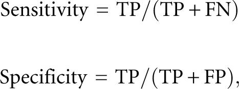 |
where TP, FN, and FP are the number of true positives, false negatives, and false positives, respectively. Figure 3 is an accuracy plot in which the prediction performances of the HMM trained using all features, as well as subsets of them, are shown. In the figure, the features calculated from the base pair probability (BPP)—that is, PL, PR, and V′—are grouped and denoted by BPP. Among the three features (CS, Z-score, and BPP), the most informative one was CS, although its prediction performance was impractical unless it was combined with the other features. Combining the Z-score and BPP improved the prediction performance compared with that of the individual feature (Fig. 3, hashed line), indicating that integrating different types of secondary structural features helps to distinguish miRNA hairpin structures. Any other combination of two features improved the prediction performance. However, combining all the features showed the highest performance.
FIGURE 3.

Specificity and sensitivity for the test data. (CS) Conservation score, (Z) Z-score, (BPP) combination of the stem potentials (PL, PR) and the loop potential (V′).
Genome scanning and comparison with other methods
We scanned the human genome sequence by using a HMM trained with all features. Figure 4 shows the number of detected miRNAs (coverage) and the total number of predictions. In this figure, our method is denoted by miRRim. The exact numbers and genomic coordinates of miRNAs predicted by miRRim are shown in Supplemental Table S1. In order to count the coverage, we enumerated the overlaps between known and predicted miRNAs. The overlap was strand-insensitive because the symmetric structures of miRNAs make it difficult to predict their orientations. An algorithm called RNAstrand (Reiche and Stadler 2007) has recently been published that predicts the orientation of noncoding RNAs based on the difference in G–U base-pair content and secondary structural stability. When one would like to know the orientation of predicted miRNA, a specialized algorithm such as this may help. The prediction performances of Berezikov et al. (2005), miRNAMap (Hsu et al. 2006), RNAmicro (Hertel and Stadler 2006), and Li et al. (2006) are also shown in Figure 4. The data on miRNAs predicted by those methods were obtained from the respective investigators' Web sites, with the exception of RNAmicro. We examined RNAmicro version 1.1 by following the procedure described by Hertel and Stadler (2006). Briefly, we applied RNAmicro to >200,000 alignment slices where RNAz scored >0.5. We evaluated three different window sizes (70, 110, and 130 bp) to scan these alignment slices. A positive hit on any window size was a miRNA candidate. All the parameters other than window size were set to default values.
FIGURE 4.

Number of miRNA detected and total number of predictions.
With miRRim, the total number of predictions was smaller than those of the other methods when the coverage was the same. The coverage of Li et al. (2006) was considerably lower than the other methods because their method is specific to intron regions and EST regions. If the coverage was adjusted to that of Berezikov's method, miRRim produces 545 predictions, of which 281 (52%), 195 (36%), 30 (5%), and 39 (7%) were within intergenic regions, intron regions, UTRs, and protein-coding regions, respectively. Those percentages are similar to those of known miRNAs (57%, 39%, 3%, and 1%, respectively). Table 1 shows the overlap matrix, which represents the number of overlaps and the percentage of overlap between two methods. The percentage overlaps among Li et al. (2006) and the other methods were relatively low. This may be because their method concentrated on intron and EST regions. The percentage overlap was only 54.3% at most between miRRim and RNAmicro, which is not so large considering the fact that similar types of features were used in both methods. Therefore, it can be said that the algorithm used to predict miRNAs markedly affected the overall result.
TABLE 1.
Overlap matrix between pairs of methods

Comparison between predicted miRNAs and known miRNAs
Among the 545 predictions by miRRim, 333 predictions did not overlap with known miRNAs. Because known miRNAs are often clustered in the genome and/or are similar to each other, we investigated genomic distance and similarity of the predicted miRNAs to known miRNAs. Table 2 summarizes the predicted miRNAs that are adjacent (within 2.5 kb) or similar (e-value ≤0.001) to known miRNAs. We performed similarity searches between human miRNA sequences in miRBase 8.2 and the predicted miRNAs by using NCBI Blastn. As shown in Table 2, 10 predictions are found to be adjacent to known miRNAs, and seven predictions are similar to known miRNAs. Among them, four predictions are both adjacent and similar to known miRNAs. The four predictions are the most hopeful candidates in terms of relative distance and similarity to known miRNAs. Actually, three of them are also predicted by other methods, supporting our predictions. The remaining one, “miRRim674,” is predicted only by our method.
TABLE 2.
Predicted miRNAs that are adjacent or similar to known miRNA

Genomic location and propensity for hairpin formation
Among the 333 predictions, 183 (55%), 99 (30%), 14 (4%), and 37 (11%) were found inside intergenic, intronic, UTR, and protein-coding regions, respectively. Thus, most predicted miRNAs are located in intergenic and intronic regions, although predicted miRNAs overlap with protein coding regions more frequently than known miRNAs (1% of known miRNAs are in protein-coding regions). The predicted miRNAs inside protein coding regions may be false positives, because most protein coding regions overlapping with predicted miRNAs are confidently annotated regions.
Next, we investigated if the predicted miRNAs, as well as corresponding conserved regions in other species, can form stable hairpin structures. A given sequence is considered to form a stable hairpin structure if at least one hairpin structure with minimum free energy lower than −25 kcal/mol is found among the potential secondary structures enumerated by RNALfold (with −L 100 option). Conserved miRNA regions in mouse, rat, and dog were obtained from the UCSC genome browser. Figure 5 shows the distribution of the number of species (Human/Mouse/Rat/Dog) in which known or predicted miRNA regions can form stable hairpin structures. For known miRNAs, ∼94% can form stable hairpin structures in at least three species. For predicted miRNAs, this percentage is ∼68%. Because miRRim's algorithm allows weak hairpin structures, some of the regions predicted by miRRim may show weak propensity for stable hairpins.
FIGURE 5.

Distribution of the number of species (Human/Mouse/Rat/Dog) in which conserved miRNA region can form a stable hairpin structure.
DISCUSSION
We developed a new method, called miRRim, for detecting miRNAs using HMMs in which evolutionary and secondary structural features around the miRNAs were used to train the HMMs. By combining evolutionary and secondary structural features, prediction performance was greatly enhanced. Although similar features are used in other methods, our method produced fewer predictions when the number of known miRNAs detected was adjusted to be the same. Moreover, there are several candidates predicted only by our method that are clustered with other miRNAs.
Because we use only evolutionary and secondary structural information to detect miRNAs, one might suspect that conserved hairpin structures other than miRNAs would be contained in our results. To address this issue, we mapped known noncoding RNAs (ncRNAs) in the Rfam database (Griffiths-Jones et al. 2005) and compared them with our results. No overlap was found between the mapped ncRNAs and our results (data not shown). It is possible that the structural features of, and the evolutionary constraints on, the miRNAs are different from those of other hairpin structures such as iron-responsive elements (Sanchez et al. 2006) and selenocysteine insertion sequences (Kryukov et al. 2003).
Several methods for detecting miRNA have been published that incorporate nucleotide sequence features. Yousef et al. (2006) used short oligonucleotide frequencies as one of the features of their naive Bayes classifier. In SVM-based methods, the frequency of short oligonucleotides with secondary structure annotations (Xue et al. 2005), and the G+C content (Hertel and Stadler 2006), were used. However, our preliminary experiment indicates that the prediction accuracy is not improved by simply adding the nucleotide content and/or the frequency of short nucleotides (data not shown). Recently, Miranda et al. (2006) reported a novel approach for predicting miRNAs based on nucleotide sequence patterns overrepresented in mature miRNA sequences. They estimated that >55,000 miRNAs exist in human genome. This estimate might be generous considering the number of miRNAs that has been discovered until now is only ∼500. However, their method is a good example to show how to incorporate nucleotide sequence features.
It is worth focusing on the performance of our method for nonconserved miRNAs that might have functions specific to humans. As seen in Figure 3, conservation scores (CSs) contribute considerably to the detection accuracy of our method. Actually, when we scanned the human genome using HMMs trained without CS, we obtained 1459 predictions, including only nine annotated miRNAs that were not conserved (mean CS <0.4). One possible way to improve the prediction performance is to integrate additional features such as nucleotide sequence features, the tendencies for miRNAs to form clusters in the genome, and homology among miRNAs.
MATERIALS AND METHODS
Training data
We used conserved miRNAs and their surrounding regions (50 bp upstream and downstream) as training data. This size of the surrounding region is chosen because the distance between two adjacent miRNAs is >50 bp for most miRNA clusters (the distance distribution between miRNAs is shown in Supplemental Fig. S5). To obtain reasonable criteria for conservation, we used a conservation score (CS) obtained from the UCSC genome browser (http://genome.ucsc.edu/). The CS is a measure of conservation and is calculated from a multiple alignment by an algorithm called phylo-HMM. Mathematically, CS is a posterior probability where a position in a multiple alignment is generated from the “conservation state” of phylo-HMM. Therefore, each nucleotide in the human genome has a CS (for details see Siepel et al. 2005). We mapped miRNA sequences from miRBase 8.2 (Griffiths-Jones et al. 2006) to the human genome (hg17) and calculated the mean CS for each mapped miRNA region including 50 bp upstream and downstream. The distribution of the mean CS showed two peaks (Fig. 6). On the basis of this distribution, we considered a miRNA with mean CS >0.4 as a conserved miRNA. Of 464 miRNA regions, 290 miRNAs met this threshold and were used as training samples.
FIGURE 6.

Distribution of mean conservation scores of miRNA regions including 50 bp upstream and downstream.
For non-miRNA training samples, we used three types of genomic regions: nonconserved, moderately conserved, and highly conserved. We randomly picked genomic regions and, according to their mean CSs, we categorized them into three categories: nonconserved (CS <0.4), moderately conserved (CS ≥0.4 and CS <0.6), and highly conserved (CS ≥0.6). For each category, we randomly selected 1000 regions with length 200 bp and used them as training samples.
Continuous HMM
We used HMMs with multivariate continuous probability density functions to model the genomic sequence features. The most general way of representing a continuous observation density is a finite mixture of normal distributions:
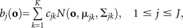 |
where o is the observation vector being modeled, cjk is the mixture coefficient for the kth mixture in state j, and N(o,μ,Σ) is typically the Gaussian probability density function with mean vector μ jk and covariance matrix Σ jk for the kth mixture component in state j. The mixture weights cjk satisfy the stochastic constraints
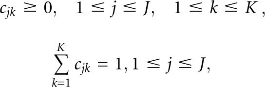 |
so that the integral of the probability density function is normalized to be 1 and the Gaussian probability density function N(o,μ,Σ) is formulated as
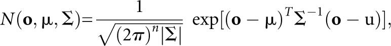 |
where n is the dimensionality of o. HMMs having this type of probability density function are called “continuous HMMs” in short. The Baum–Welch (Baum 1972) and Viterbi decoding (Viterbi 1967) algorithms have been shown to be applicable to continuous HMMs, as well as HMMs with discrete probabilities, without loss of mathematical rigor (Rabiner and Juang 1993).
Training continuous HMMs
In our method, each training sample is represented by a feature vector sequence S=o 1, o 2, o 3…o l, where l is the nucleotide length of the training sample and o i is a feature vector consisting of evolutionary and secondary structural features. We used the hidden Markov model toolkit (HTK) available at http://htk.eng.cam.ac.uk/ to train miRNA and non-miRNA models. For a miRNA model, we first consider a HMM in which all states are linearly connected (Fig. 7A). Since this architecture can generate vector sequences of infinite length, we introduce a restriction on the number of self-loops for this architecture (Fig. 7B). The architecture contains 50 state groups, each of which contains six states connected as shown in the figure. The six states in a state group are “tied;” i.e., they have the same probability density function. Thereby, the number of parameters of the model does not increase compared with a model containing 50 linearly connected states, like in Figure 7A. Because two to six states must be traversed in each state group, the length of vector sequences that can fit this architecture is restricted to be from 2 × 50 to 6 × 50. We introduce these length restrictions because the minimum and maximum lengths of miRNA training samples are 160 and 236 bp, respectively. The number of state groups, 50, was chosen based on investigation of the prediction performance of our method (see supplemental information). More complex architectures can be used. For example, each state group can have a different number of tied states. Such architectures might reflect the length variation in stem, loop, and surrounding regions, separately. However, when we evaluated several types of complex architectures, overall performance was not improved. Therefore, we chose the relatively simple architecture shown in Figure 7B.
FIGURE 7.

Architectures and transition probabilities of Hidden Markov models. (Circled “s”) Start state, (circled “e”) end state. (A) An architecture with linearly connected states, (B) an architecture for a miRNA model that consists of 50 state groups, (C) transition probabilities between states within a state group, (D) an architecture for non-miRNA models.
The transition probabilities are initialized as in Figure 7C, so that accumulating them over any state sequence in a state group always results in a probability of one-fifth. The probabilities are not changed by the training procedure, because our training data are insufficient for estimating the state group length distribution modeled in this way. The emission probability of each state follows a mixture distribution consisting of two normal distributions having diagonal covariance matrices in which all covariance factors are set to zero except the diagonal factors. The means μ jk, variances Σjk = diag(σ 1 2, σ 2 2 … σ n 2), and weights of the mixture distribution cjk in each state are first optimized by the Viterbi training algorithm (Rabiner and Juang 1993) and then re-estimated by the Baum-Welch algorithm.
For non-miRNA models, we construct three HMMs corresponding to nonconserved, moderately conserved, and highly conserved regions. Each model is learned by a single-state HMM containing a self-loop transition probability (Fig. 7D). The emission probability of the state follows a mixture distribution consisting of five normal distributions again having a diagonal covariance matrix. The means, variances, and weights of the mixture distribution, as well as the transition probabilities, are first optimized by the Viterbi training algorithm and then re-estimated by the Baum–Welch algorithm.
Scanning genomic sequence by trained HMMs
A miRNA model and the non-miRNA models are connected into a single HMM, in which the states both in the miRNA model and the non-miRNA models can be visited in turn (Fig. 2). Before a long genomic region is scanned, the region is converted into a feature vector sequence by the same procedure used on the training samples. Using the Viterbi decoding algorithm, the vector sequence is scanned, and the sequence segments that are aligned to the miRNA model are considered to be miRNA regions. The balance between sensitivity and specificity is controlled by modifying the probability of transition τ from the non-miRNA models to the miRNA model.
Feature vectors
Each training sample is represented by a feature vector sequence S=o 1, o 2, o 3…o l, where l is the length of the training sample and o i is a five-dimensional feature vector in which one dimension is the conservation score (CS) and the remaining four are the secondary structural features. Of the four dimensions, one is the Z-score, and the remaining three are the stem and loop potentials calculated from the base pair probability.
Z-score
The Z-score of a given sequence is calculated by the following equation:
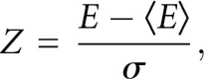 |
where E is the MFE of a given sequence and 〈E〉 and σ are the mean and the standard deviation, respectively, of the MFE calculated from randomly generated sequences that have the same length and base composition. Because calculating 〈E〉 and σ every time is time consuming, Washietl et al. (2005) used SVM regression to infer these values and have shown that the accuracy of the regression was very high. We used the method of Washietl et al. (2005) to calculate Z-scores quickly. We scanned each training sample using a 100-bp window. The Z-score at position i of a training sample is calculated at the window from i–49 to i+50.
Stem potential
The stem potential is calculated based on the base pair probability. The base pair probability, pij, represents the probability that positions i and j form a base pair, and it can be calculated by McCaskill's algorithm (McCaskill 1990). We obtain the base pair probability matrix of each training sample by using the RNAplfold program (Bernhart et al. 2006) with a window size of 120 bp. When pij is close to 1 and i<j, positions i and j are likely to become the left and right sides, respectively, of a base pair. We define the probability that a base at position i becomes the left or right side of a base pair, PiL and PiR, by the following equations:
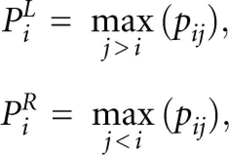 |
where pij is the base pair probability between i and j. PiL and PiR are considered to represent the stem potential, because their values become high in the stem region. Using the above two equations, we can convert a base pair probability matrix into two-dimensional vectors. The same representation is used in the RNApdist algorithm (Bonhoeffer et al. 1993), except that the sum function is used instead of the max function in miRRim.
Loop potential
The loop potential is calculated from the base pair probability. We first define the unweighted loop potential as follows:
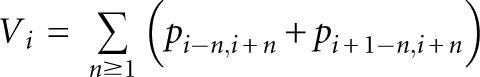 |
We further apply a triangular weighting to Vi as follows:
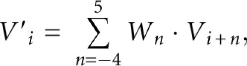 |
where W −4…+5 = {1/30, 2/30, 3/30, 4/30, 5/30, 4/30, 3/30, 2/30, 1/30}. The value of V′i becomes high when position i is around the center of the terminal loop of the hairpin structure containing symmetric bulges or no bulge.
Effects of changing parameters
In this section, we summarize the influence of changing (1) the length of upstream and downstream regions contained in miRNA training samples; (2) the number of state groups in the architecture of the miRNA model; and (3) the number of mixture components in miRNA and non-miRNA models. We changed these parameters and evaluated the performance of our method. We observed that:
(1) The prediction performance was higher when upstream and downstream regions were included in training samples than when only miRNA hairpins were included (Supplemental Fig. S1). HMMs trained using training samples with 75 or 100 bp upstream and downstream regions missed the prediction of clustered miRNAs. Therefore, using 25 or 50 bp is appropriate.
(2) The prediction accuracy was not so affected by changing the number of state groups. An architecture containing at least 20 state groups was sufficient for accurate prediction (Supplemental Fig. S2).
(3) For a miRNA model, using a mixture of two or three components is better than a single Gaussian (Supplemental Fig. S3). For non-miRNA models, using a mixture of more than three components is better than that of one to three components (Supplemental Fig. S4).
Details are described in supplemental information.
SUPPLEMENTAL DATA
Genomic coordinates of predicted miRNA (Supplemental Table S1), programs to find miRNA, details on effects of changing parameters (Supplemental Figs. S1–4), and the distance distribution between miRNAs (Supplemental Fig. S5) can be obtained from http://mirrim.ncrna.org/.
ACKNOWLEDGMENTS
This work was supported by the Functional RNA Project of the New Energy and Industrial Technology Development Organization (NEDO). We thank members of the bioinformatics group at the National Institute of Advanced Industrial Science and Technology (AIST) and the members of the Japan Biological Information Consortium (JBIC) for useful discussions.
Footnotes
Article published online ahead of print. Article and publication date are at http://www.rnajournal.org/cgi/doi/10.1261/rna.655107.
REFERENCES
- Baum, L.E. An equality and associated maximization technique in statistical estimation for probabilistic functions of Markov processes. Inequalities. 1972;3:1–8. [Google Scholar]
- Berezikov, E., Guryev, V., van de Belt, J., Wienholds, E., Plasterk, R.H., Cuppen, E. Phylogenetic shadowing and computational identification of human microRNA genes. Cell. 2005;120:21–24. doi: 10.1016/j.cell.2004.12.031. [DOI] [PubMed] [Google Scholar]
- Bernhart, S.H., Hofacker, I.L., Stadler, P.F. Local RNA base pairing probabilities in large sequences. Bioinformatics. 2006;22:614–615. doi: 10.1093/bioinformatics/btk014. [DOI] [PubMed] [Google Scholar]
- Bonhoeffer, S., McCaskill, J.S., Stadler, P.F., Schuster, P. RNA multi-structure landscapes. A study based on temperature dependent partition functions. Eur. Biophys. J. 1993;22:13–24. doi: 10.1007/BF00205808. [DOI] [PubMed] [Google Scholar]
- Calin, G.A., Dumitru, C.D., Shimizu, M., Bichi, R., Zupo, S., Noch, E., Aldler, H., Rattan, S., Keating, M., Rai, K., et al. Frequent deletions and down-regulation of micro-RNA genes miR15 and miR16 at 13q14 in chronic lymphocytic leukemia. Proc. Natl. Acad. Sci. 2002;99:15524–15529. doi: 10.1073/pnas.242606799. [DOI] [PMC free article] [PubMed] [Google Scholar]
- Calin, G.A., Sevignani, C., Dumitru, C.D., Hyslop, T., Noch, E., Yendamuri, S., Shimizu, M., Rattan, S., Bullrich, F., Negrini, M., et al. Human microRNA genes are frequently located at fragile sites and genomic regions involved in cancers. Proc. Natl. Acad. Sci. 2004;101:2999–3004. doi: 10.1073/pnas.0307323101. [DOI] [PMC free article] [PubMed] [Google Scholar]
- Griffiths-Jones, S., Moxon, S., Marshall, M., Khanna, A., Eddy, S.R., Bateman, A. Rfam: Annotating noncoding RNAs in complete genomes. Nucleic Acids Res. 2005;33:D121–D124. doi: 10.1093/nar/gki081. [DOI] [PMC free article] [PubMed] [Google Scholar]
- Griffiths-Jones, S., Grocock, R.J., van Dongen, S., Bateman, A., Enright, A.J. miRBase: microRNA sequences, targets, and gene nomenclature. Nucleic Acids Res. 2006;34:D140–D144. doi: 10.1093/nar/gkj112. [DOI] [PMC free article] [PubMed] [Google Scholar]
- Hertel, J., Stadler, P.F. Hairpins in a haystack: Recognizing microRNA precursors in comparative genomics data. Bioinformatics. 2006;22:e197–e202. doi: 10.1093/bioinformatics/btl257. [DOI] [PubMed] [Google Scholar]
- Hofacker, I.L., Bernhart, S.H., Stadler, P.F. Alignment of RNA base pairing probability matrices. Bioinformatics. 2004;20:2222–2227. doi: 10.1093/bioinformatics/bth229. [DOI] [PubMed] [Google Scholar]
- Hsu, P.W., Huang, H.D., Hsu, S.D., Lin, L.Z., Tsou, A.P., Tseng, C.P., Stadler, P.F., Washietl, S., Hofacker, I.L. miRNAMap: Genomic maps of microRNA genes and their target genes in mammalian genomes. Nucleic Acids Res. 2006;34:D135–D139. doi: 10.1093/nar/gki081. [DOI] [PMC free article] [PubMed] [Google Scholar]
- John, B., Enright, A.J., Aravin, A., Tuschl, T., Sander, C., Marks, D.S. Human MicroRNA targets. PLoS Biol. 2004;2:e363. doi: 10.1371/journal.pbio.0020363. [DOI] [PMC free article] [PubMed] [Google Scholar]
- Krek, A., Grun, D., Poy, M.N., Wolf, R., Rosenberg, L., Epstein, E.J., MacMenamin, P., da Piedade, I., Gunsalus, K.C., Stoffel, M., et al. Combinatorial microRNA target predictions. Nat. Genet. 2005;37:495–500. doi: 10.1038/ng1536. [DOI] [PubMed] [Google Scholar]
- Kryukov, G.V., Castellano, S., Novoselov, S.V., Lobanov, A.V., Zehtab, O., Guigo, R., Gladyshev, V.N. Characterization of mammalian selenoproteomes. Science. 2003;300:1439–1443. doi: 10.1126/science.1083516. [DOI] [PubMed] [Google Scholar]
- Lai, E.C., Tomancak, P., Williams, R.W., Rubin, G.M. Computational identification of Drosophila microRNA genes. Genome Biol. 2003;4:R42. doi: 10.1186/gb-2003-4-7-r42. [DOI] [PMC free article] [PubMed] [Google Scholar]
- Lee, Y., Jeon, K., Lee, J.T., Kim, S., Kim, V.N. MicroRNA maturation: Stepwise processing and subcellular localization. EMBO J. 2002;21:4663–4670. doi: 10.1093/emboj/cdf476. [DOI] [PMC free article] [PubMed] [Google Scholar]
- Legendre, M., Lambert, A., Gautheret, D. Profile-based detection of microRNA precursors in animal genomes. Bioinformatics. 2005;21:841–845. doi: 10.1093/bioinformatics/bti073. [DOI] [PubMed] [Google Scholar]
- Lewis, B.P., Burge, C.B., Bartel, D.P. Conserved seed pairing, often flanked by adenosines, indicates that thousands of human genes are microRNA targets. Cell. 2005;120:15–20. doi: 10.1016/j.cell.2004.12.035. [DOI] [PubMed] [Google Scholar]
- Li, S.C., Pan, C.Y., Lin, W.C. Bioinformatic discovery of microRNA precursors from human ESTs and introns. BMC Genomics. 2006;7:164. doi: 10.1186/1471-2164-7-164. [DOI] [PMC free article] [PubMed] [Google Scholar]
- Lim, L.P., Lau, N.C., Weinstein, E.G., Abdelhakim, A., Yekta, S., Rhoades, M.W., Burge, C.B., Bartel, D.P. The microRNAs of Caenorhabditis elegans . Genes & Dev. 2003;17:991–1008. doi: 10.1101/gad.1074403. [DOI] [PMC free article] [PubMed] [Google Scholar]
- McCaskill, J.S. The equilibrium partition function and base pair binding probabilities for RNA secondary structure. Biopolymers. 1990;29:1105–1119. doi: 10.1002/bip.360290621. [DOI] [PubMed] [Google Scholar]
- Metzler, M., Wilda, M., Busch, K., Viehmann, S., Borkhardt, A. High expression of precursor microRNA-155/BIC RNA in children with Burkitt lymphoma. Genes Chromosomes Cancer. 2004;39:167–169. doi: 10.1002/gcc.10316. [DOI] [PubMed] [Google Scholar]
- Michael, M.Z., O'Connor, S.M., van Holst Pellekaan, N.G., Young, G.P., James, R.J. Reduced accumulation of specific microRNAs in colorectal neoplasia. Mol. Cancer Res. 2003;1:882–891. [PubMed] [Google Scholar]
- Miranda, K.C., Huynh, T., Tay, Y., Ang, Y.S., Tam, W.L., Thomson, A.M., Lim, B., Rigoutsos, I. A pattern-based method for the identification of MicroRNA binding sites and their corresponding heteroduplexes. Cell. 2006;126:1203–1217. doi: 10.1016/j.cell.2006.07.031. [DOI] [PubMed] [Google Scholar]
- Nam, J.W., Shin, K.R., Han, J., Lee, Y., Kim, V.N., Zhang, B.T. Human microRNA prediction through a probabilistic co-learning model of sequence and structure. Nucleic Acids Res. 2005;33:3570–3581. doi: 10.1093/nar/gki668. [DOI] [PMC free article] [PubMed] [Google Scholar]
- Ohler, U., Yekta, S., Lim, L.P., Bartel, D.P., Burge, C.B. Patterns of flanking sequence conservation and a characteristic upstream motif for microRNA gene identification. RNA. 2004;10:1309–1322. doi: 10.1261/rna.5206304. [DOI] [PMC free article] [PubMed] [Google Scholar]
- Rabiner, L., Juang, B.H. Fundamentals of speech recognition. Prentice-Hall Inc; Englewood Cliffs, NJ: 1993. Chapter 6, Theory and implementation of Hidden Markov Models; pp. 321–389. [Google Scholar]
- Reiche, K., Stadler, P.F. RNAstrand: Reading direction of structured RNAs in multiple sequence alignments. Algorithms Mol. Biol. 2007;2:6. doi: 10.1186/1748-7188-2-6. [DOI] [PMC free article] [PubMed] [Google Scholar]
- Ruby, J.G., Jan, C.H., Bartel, D.P. Intronic microRNA precursors that bypass Drosha processing. Nature. 2007;448:83–86. doi: 10.1038/nature05983. [DOI] [PMC free article] [PubMed] [Google Scholar]
- Sanchez, M., Galy, B., Dandekar, T., Bengert, P., Vainshtein, Y., Stolte, J., Muckenthaler, M.U., Hentze, M.W. Iron regulation and the cell cycle: Identification of an iron-responsive element in the 3′-untranslated region of human cell division cycle 14A mRNA by a refined microarray-based screening strategy. J. Biol. Chem. 2006;281:22865–22874. doi: 10.1074/jbc.M603876200. [DOI] [PubMed] [Google Scholar]
- Scott, G.K., Goga, A., Bhaumik, D., Berger, C.E., Sullivan, C.S., Benz, C.C. Coordinate suppression of ERBB2 and ERBB3 by enforced expression of micro-RNA miR-125a or miR-125b. J. Biol. Chem. 2007;282:1479–1486. doi: 10.1074/jbc.M609383200. [DOI] [PubMed] [Google Scholar]
- Sewer, A., Paul, N., Landgraf, P., Aravin, A., Pfeffer, S., Brownstein, M.J., Tuschl, T., van Nimwegen, E., Zavolan, M. Identification of clustered microRNAs using an ab initio prediction method. BMC Bioinformatics. 2005;6:267. doi: 10.1186/1471-2105-6-267. [DOI] [PMC free article] [PubMed] [Google Scholar]
- Siepel, A., Bejerano, G., Pedersen, J.S., Hinrichs, A.S., Hou, M., Rosenbloom, K., Clawson, H., Spieth, J., Hillier, L.W., Richards, S., et al. Evolutionarily conserved elements in vertebrate, insect, worm, and yeast genomes. Genome Res. 2005;15:1034–1050. doi: 10.1101/gr.3715005. [DOI] [PMC free article] [PubMed] [Google Scholar]
- Song, L., Tuan, R.S. MicroRNAs and cell differentiation in mammalian development. Birth Defects Res. C Embryo Today. 2006;78:140–149. doi: 10.1002/bdrc.20070. [DOI] [PubMed] [Google Scholar]
- Viterbi, A.J. Error bounds for convolutional codes and an asymptotically optimum decoding algorithm. IEEE Trans. Inf. Theory. 1967;13:260–269. [Google Scholar]
- Wang, X., Zhang, J., Li, F., Gu, J., He, T., Zhang, X., Li, Y. MicroRNA identification based on sequence and structure alignment. Bioinformatics. 2005;21:3610–3614. doi: 10.1093/bioinformatics/bti562. [DOI] [PubMed] [Google Scholar]
- Washietl, S., Hofacker, I.L., Stadler, P.F. Fast and reliable prediction of noncoding RNAs. Proc. Natl. Acad. Sci. 2005;102:2454–2459. doi: 10.1073/pnas.0409169102. [DOI] [PMC free article] [PubMed] [Google Scholar]
- Xie, X., Lu, J., Kulbokas, E.J., Golub, T.R., Mootha, V., Lindblad-Toh, K., Lander, E.S., Kellis, M. Systematic discovery of regulatory motifs in human promoters and 3′ UTRs by comparison of several mammals. Nature. 2005;434:338–345. doi: 10.1038/nature03441. [DOI] [PMC free article] [PubMed] [Google Scholar]
- Xue, C., Li, F., He, T., Liu, G.P., Li, Y., Zhang, X. Classification of real and pseudo microRNA precursors using local structure-sequence features and support vector machine. BMC Bioinformatics. 2005;6:310. doi: 10.1186/1471-2105-6-310. [DOI] [PMC free article] [PubMed] [Google Scholar]
- Yousef, M., Nebozhyn, M., Shatkay, H., Kanterakis, S., Showe, L.C., Showe, M.K. Combining multispecies genomic data for microRNA identification using a Naive Bayes classifier. Bioinformatics. 2006;22:1325–1334. doi: 10.1093/bioinformatics/btl094. [DOI] [PubMed] [Google Scholar]