The free energy landscape of small peptides as obtained from metadynamics with umbrella sampling corrections

Abstract

There is considerable interest in developing methodologies for the accurate evaluation of free energies, especially in the context of biomolecular simulations. Here, we report on a reexamination of the recently developed metadynamics method, which is explicitly designed to probe “rare events” and areas of phase space that are typically difficult to access with a molecular dynamics simulation. Specifically, we show that the accuracy of the free energy landscape calculated with the metadynamics method may be considerably improved when combined with umbrella sampling techniques. As test cases, we have studied the folding free energy landscape of two prototypical peptides: Ace-(Gly)₂-Pro-(Gly)₃-Nme in vacuo and trialanine solvated by both implicit and explicit water. The method has been implemented in the classical biomolecular code AMBER and is to be distributed in the next scheduled release of the code. © 2006 American Institute of Physics.

I. INTRODUCTION

The accurate determination of free energies can be quite challenging, both experimentally and theoretically. A large number of numerical methods has been developed for the evaluation of free energies¹ during the last few decades, many of them involving Monte Carlo or molecular dynamics (MD) methods (or combinations thereof) at different levels of theoretical approximation (quantum, classical atomistic, coarse-grained descriptions, etc.). Naturally, as polyatomic systems become more complex, it generally becomes computationally more challenging to estimate the free energies of various (meta) stable configurations and/or to accelerate rare events. In particular, a straightforward application of MD, for instance, to sample the canonical distribution of the system is typically doomed to failure since the MD trajectory will be either trapped in the neighborhood of a potential energy minimum or locked in some region of the phase space due to entropic bottlenecks.

Many methods are therefore being developed to accelerate the dynamics and sampling of rare events in the context of atomistic simulations. The methods usually employed fall into two general categories: (i) those that add biasing terms to the original potential energy (this typically requires the definition of an appropriate order parameter), such as umbrella sampling methods and adaptive-force bias method;² (ii) those that consider a generalized ensemble³ of the original system and exploit enhanced sampling, e.g., at different temperatures, such as replica exchange molecular dynamics (REMD), also known as parallel tempering.^4,5 Sampling in the latter is usually canonical, which means that the states beyond a few k_BT are seldom visited—if ever—so that the barrier height determination is plagued by statistical errors.

In the umbrella sampling methods, the biasing potential is usually a function of a low-dimensional collective variable, which means that the majority of the (hopefully irrelevant) degrees of freedom are de facto integrated out. The unbiased probabilities of the collective variable can then be easily recovered from the biased simulation. In order to do so, two strategies are typically in use: (i) running a number of biased simulations, each exploring a slightly different range of the collective variables, and then gluing them together using the weighted histogram analysis method (WHAM);⁶ (ii) running biased simulations sequentially using the probabilities collected after each stage to build improved biasing potentials to be used in the next run (the so-called adaptive umbrella sampling^7-10). If it comes to canonical distribution sampling, the umbrellalike methods are obviously less general than those exploiting generalized ensembles; however, they can naturally explore rare states. For the umbrellalike methods, the right choice of the collective variable is of paramount importance.

An interesting variation of the adaptive umbrella sampling method, the metadynamics method, has been recently proposed in Refs. ¹¹ and ¹². The metadynamics method is based on the extended Lagrangian ideas and coarse-grained non-Markovian dynamics.^13-15 It allows for different pathways to explore rare events in systems with complex potential energy surfaces. The method is also closely related to the local elevation method,¹⁶ to the adaptive-force bias method,² to coarse molecular dynamics,¹⁷ and to the Wang-Landau approach.¹⁸ When combined with Car-Parrinello dynamics, the metadynamics method can explore complex reaction paths involving several energy barriers at relatively modest computational costs.^19-27

In order to test the metadynamics method for classical biomolecular simulations and to make it available to the general public, we have implemented it in the classical MD code AMBER 8 (Ref. ²⁸) and plan to distribute it in the next release of AMBER. In this work we report on some improvements made with respect to the original implementation and apply the method to explore the free energy surfaces of two small, prototypical peptides. Studies of the metadynamics method have shown that one of the associated weakness of the method (a weakness that remains, in spite of having been addressed before) is the lack of a reliable free energy error estimate. In order to improve the method's accuracy, in this work we employ biased MD to validate and improve the free energy estimates obtained by the metadynamics method.

As test cases, we explore the free energy landscape of two model peptides, Ace-(Gly)₂-Pro-(Gly)₃-Nme in vacuo which can display a β-hairpin folded conformation and zwitterionic trialanine, both in implicit and explicit solvent, which exhibits an α-helix-like structure. Understanding the underlying mechanisms that drive protein folding is still an open challenge for the scientific community. Peptides offer a more approachable system than proteins because they fold at very fast rates and can therefore give an insight into the early stages of protein folding. Furthermore, the development of fast time-resolved spectroscopy allows for an exciting, direct comparison between the experimental folding of the peptide and the folding as obtained with MD simulations. In addition, new and revisited sampling techniques help to better explore the peptide conformational landscape (for a review see Ref. 29). In general, these sampling methods have been applied to only short peptides.^30-32 The reasons for this depend on the type of method. For umbrellalike methods, the definition of the relevant order parameter, capable of capturing the complex tertiary structure of a protein, can be daunting due to the huge number of degrees of freedom that vary concurrently as the protein folds.³² For the pure (not biased) REMD-like methods, sampling is canonical and therefore transition states are seldom visited.

The paper is organized as follows. In the next section we review the methods used and briefly describe our implementation. In Sec. III, we provide technical details of the simulations. The application of the method to study the free energy landscapes of the two model peptides is presented in Sec. IV. Conclusions and outlook are contained in the last section.

II. METHODS

A. Metadynamics

Metadynamics^11,12,16 has been extensively described in the literature. Here we reformulate the description once more, so as to bring out the details of our implementation. In the spirit of umbrella sampling methods, the metadynamics method requires from the user the identification of a collective variable σ=σ(r₁, ... ,r_N), defined as a sufficiently smooth function of atomic positions r_a, a=1, ... ,N, with the values in a differentiable manifold $\mathbb{Q}$. The method provides an elegant way to compute the probability density of the collective variable,

$$p\left(\xi \right)=\langle \delta [\xi -\sigma ({\mathbf{r}}_1,\dots ,{\mathbf{r}}_N)]\rangle ,$$ (2.1)

and the associated free energy,

$$f\left(\xi \right)=-k_{B}T\ln p\left(\xi \right).$$ (2.2)

The angular brackets here denote the ensemble average, k_B is the Boltzmann constant, and T is the temperature.

The method introduces an additional dynamical variable $\eta \left(t\right)\in \mathbb{Q}$, which can be conveniently thought of as a test particle whose dynamics is designed to probe the free energy (2.2). To this end the test particle η(t) is given a mass M and coupled harmonically to the collective variable σ(r₁, ... ,r_N). Its motion is set to be governed by Newton's equation (up to temperature regulation),

$$M\frac{d^2\eta }{d{t}^2}+K[\eta -\sigma ({\mathbf{r}}_1,\dots ,{\mathbf{r}}_N)]=0,\eta \in \mathbb{Q},$$ (2.3)

where for multidimensional $\mathbb{Q}$ each component of η(t) can have a different mass and spring constant K. The harmonic term in Eq. (2.3) is inspired by the Gaussian approximation of the Dirac δ function in Eq. (2.1),

$$\frac{\partial }{\partial \eta }\ln \delta (\eta -\sigma )\approx \frac{\partial }{\partial \eta }\ln \exp \left[-\frac{K}{2}{(\eta -\sigma )}^2\right],$$

such that the free energy gradient drives the dynamics of η(t). Indeed, if M is large enough to ensure that the dynamics of η(t) is much slower than the dynamics of the microscopic degrees of freedom and the latter dynamics is ergodic, the ensemble average in Eq. (2.1) can be approximated by a time average on the time scale set by the dynamics of η(t). The test particle thus probes the free energy (2.2).

The dynamics of η(t) is then used to build a time-dependent biasing potential, V_h (referred to as hill potential in what follows), meant to force the system to explore as of yet unexplored regions of $\mathbb{Q}$. The hill potential is essentially a sum of tiny hills settled along the trajectory of the test particle. The shape of the hills is not particularly important. It can be shown³³ that if certain conditions are met, the hill potential approaches the negative of the free energy within a constant in the t→∞ limit. Roughly speaking, the hills “flood” the free energy well so that the system can cross the lowest transition state to a neighboring local minimum. When all the free energy minima within the desired region of $\mathbb{Q}$ have been completely flooded, the system can move freely among the different states in this region and the free energy “portrait” within this region is given by the hill potential gathered.

In the original metadynamics formulation¹² the hill potential acts on η(t), i.e., V_h=V_h(η, t) [therefore its derivative enters in Eq. (2.3)]. This introduces an “indirection:” V_h “pushes” η(t) and η(t) then “pulls” the system by means of the harmonic coupling. We have found that, for purely classical systems, the method performs better (comparatively smaller M and K are needed), if this indirection is avoided and the hill potential is made to act directly on the microscopic degrees of freedom, i.e., V_h=V_h[σ(r₁, ... ,r_N),t]. Thus, the atomic equation of motion (up to temperature and pressure regulation) is

$$m_a\frac{d^2{\mathbf{r}}_a}{d{t}^2}+\frac{\partial }{\partial {\mathbf{r}}_a}\frac{K}{2}{[\eta -\sigma ({\mathbf{r}}_1,\dots ,{\mathbf{r}}_N)]}^2={\mathbf{F}}_a-\frac{\partial }{\partial {\mathbf{r}}_a}{V}_h[\sigma ({\mathbf{r}}_1,\dots ,{\mathbf{r}}_N),t],$$ (2.4)

where m_a are the atomic masses and F_a are the interatomic forces.

In Ref. 12 the hill potential is given by the sum of products of two Gaussians: one spherical Gaussian multiplied by one “anisotropic” Gaussian of different width that depends on the displacement between the potential hills added at different times, such that subsequently added potential hills close to each other are narrowed in the direction of the trajectory (“Gaussian tube”). We have found that the presence of the displacement-dependent Gaussians in V_h(σ,t) does not increase the accuracy of the method, but does increase the cost of the calculation.

In our implementation, the hill potential V_h(σ,t) is given by the sum (meant to approximate an integral over time) of smoothly truncated Gaussians, settled at points ${\eta }^{\left(n\right)}$ along the η(t)'s trajectory,

$$V_h(\sigma ,t)=A\sum _{n}G[R(\sigma \mid {\eta }^{\left(n\right)})∕W]∕G\left(0\right),$$ (2.5)

where A is the hill amplitude, W is the hill width, $R(\sigma \mid {\eta }^{\left(n\right)})$ is the distance between σ and ${\eta }^{\left(n\right)}$, and

$$G\left(r\right)=\{\begin{array}{cc}{e}^{-r^2∕2}+P\left(r\right)e^{-r_c^2∕2},\hfill & r<r_c\hfill \\ 0,\hfill & r\ge r_c,\hfill \end{array}\phantom{\}}P\left(r\right)=\frac{1}{2}{r}^2(1+\frac{1}{2}{r}_c^2-\frac{1}{4}{r}^2)-\frac{1}{2}{r}_c^2(1+\frac{1}{4}{r}_c^2)-1.$$ (2.6)

Here, r_c denotes the cutoff radius, which we typically set to 2 in our simulations.

If $\mathbb{Q}$ is nonsimply connected, R should be set to the shortest distance between σ and ${\eta }^{\left(n\right)}$ (and, obviously, if $\mathbb{Q}$ is nonsimply connected the width W must be reasonably small). In practice, different components of the collective variable may be scaled to make the Gaussians G(r) anisotropic. We have omitted the explicit scale factors above for clarity. For the same reason, we have also omitted the optional time dependence of the amplitudes A and widths W.

The above form of the hill potential is more suited for rapid evaluation than the one proposed in Ref. 12. This fast evaluation is achieved by distributing the Gaussians equally among all processors and organizing their positions in kd-trees³⁴ (see Appendix) such that each processor manages its own tree. The kd-trees facilitate a quick sum of all the Gaussians within the cutoff distance from a given point. For a typical simulation, the use of kd-trees leads to a noticeable speedup, but strict performance analysis in the general case is rather difficult.

A metadynamics simulation depends on several parameters, whose values have to be carefully selected. The force constant K has to be large enough to keep η(t) close to σ(r₁, ... ,r_N). However, very large values of K require a tiny time step for MD, which can become impractical. The mass M also has to be large so that the dynamics of the test particle is adiabatically decoupled from the atomic motions. However, if M is very large, the computation again becomes very slow. The accuracy and efficiency of the “flooding” procedure are determined by the amplitude A, the width W, and the “stride” between added hills τ_G. The latter actually is not a single parameter but a shorthand notation that indicates when a new Gaussian is added to the hill potential: when the displacement of the test particle in $\mathbb{Q}$ exceeds a certain limit, but not before a preset minimum number of MD steps and not beyond a maximum number of MD steps. The parameters A, W, and τ_G cannot be chosen independently. It has been claimed in Ref. 35 that increasing the width of the Gaussians requires an increase of the stride to avoid “hill surfing” (where the collective variable continuously rides the tail of the most recently placed hill) and increasing the amplitude requires increasing the width (and therefore increasing the stride) to avoid steep forces on the collective variable. However, very large strides and small hills place serious constraints on the efficiency of phase space exploration. The final efficiency and accuracy of the simulation depend therefore on an artful combination of these parameters.

B. Umbrella corrections

One of the problems of the metadynamics method that several of the original authors have addressed before is the lack of a reliable free energy error estimate. One source of error (the flooding error) has been analyzed recently in Ref. 36. The reasoning in Ref. 36 assumes that both mass M of the test particle and the harmonic coupling constant K are infinite, so that the free energy errors arising from finite M and K are effectively ignored. The resulting error estimate depends on the hill parameters A and W, the effective τ_G, as well as the temperature, the size of the explored region of $\mathbb{Q}$, and the collective variable diffusion constant. As such, it mainly assesses the “reconstruction” accuracy. Another important source of error is the inaccurate “average” in Eq. (2.1) that arises due to finite (instead of infinite) values of M and K so that the test particle may end up probing some transient energy instead of the free energy (2.2). This error is particularly problematic in situations with non-negligible entropy.

We believe that the most accurate way to determine the free energy error and, therefore, to construct a more accurate free energy approximation is to use umbrella sampling. In fact, a “recipe” for computing free energy paths was given in Ref. 35, where the authors developed a method to localize the lowest free energy path that connects two minima and expressed it in the form of a one-dimensional reaction coordinate. The potential along this one-dimensional coordinate was then used to perform umbrella sampling to correct the metadynamics results. In this work we use the whole metadynamics-generated hill potential “as is” as the biasing potential for umbrella sampling, i.e., in the spirit of adaptive umbrella sampling.⁴⁵ After running molecular dynamics with the biasing potential V_h(σ), one can calculate the biased probability density,

$$p^B\left(\xi \right)={\langle \delta [\xi -\sigma ({\mathbf{r}}_1,\dots ,{\mathbf{r}}_N)]\rangle }_B.$$ (2.7)

If, as a result of the metadynamics run, the hill potential satisfies $f\left(\xi \right)=-V_h\left(\xi \right)$ exactly, the biased probability density $p^B\left(\xi \right)$ would be flat (constant). In practice it is not flat, and $p^B\left(\xi \right)$ can thus be used to “correct” metadynamics,

$$f\left(\xi \right)=-V_h\left(\xi \right)-k_{B}T\ln p^B\left(\xi \right).$$ (2.8)

Here we note that f(ξ) also includes a ξ-independent term, not shown in the above equation. Since we work with fixed external conditions, and with only one biasing potential $V_h\left(\xi \right)$, this term is irrelevant and needs not be considered here.

III. SIMULATION DETAILS

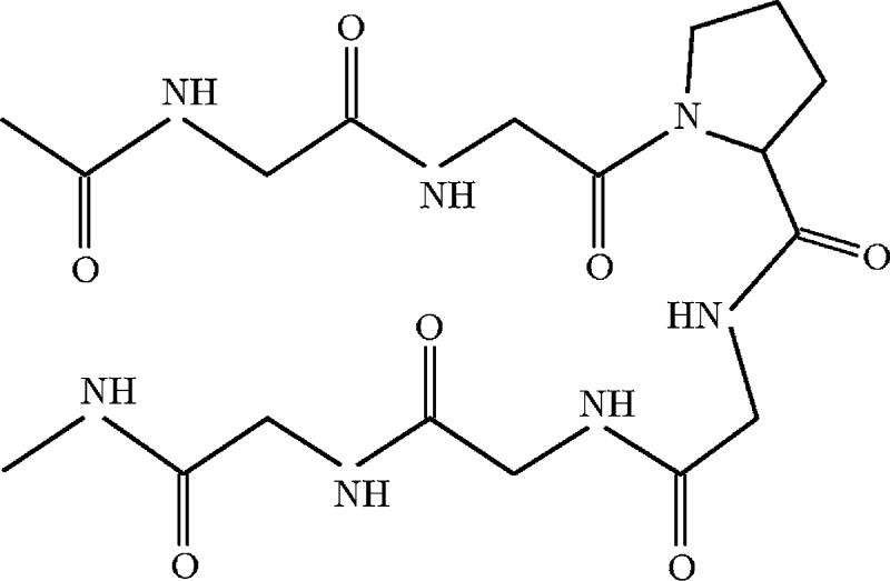
We applied the methods described in the previous section to study the configurational landscape of two model peptides, Ace-(Gly)₂-Pro-(Gly)₃-Nme (Fig. 1) and trialanine in its zwitterionic form (Fig. 2). Trialanine is studied both in implicit and explicit solvents. Ace-(Gly)₂-Pro-(Gly)₃-Nme, on the other hand, seems to be hydrophobic and its hairpin conformation unstable in solvent, so we have run it in vacuo. The details of the simulations are as follows.

FIG. 1.

Ace-(Gly)₂-Pro-(Gly)₃-Nme peptide in a β-hairpin conformation (sketch).

FIG. 2.

Trialanine with zwitterionic end groups ${\mathrm{NH}}_3^{+}$ and ${\mathrm{CO}}_2^{-}$. Also shown is the pair of dihedral angles (φ, ψ) chosen as collective variable for the metadynamics simulations.

Molecular dynamics

Initial configurations were generated using the LEAP program from the AMBER 8 package so that both peptides were completely unfolded at time zero. The simulations employed the 1999 version of the force field of Cornell et al.³⁸ The simulations were carried out at constant temperature (300 K) using the algorithm of Berendsen et al.³⁹ with a 2 fs time step and τ_T=2 ps. The SHAKE algorithm was applied to all bonds involving hydrogen atoms. The Ace-(Gly)₂-Pro-(Gly)₃-Nme peptide was run in vacuo with a 512 Å cutoff for the nonbonded interactions. Triala-nine was run both in implicit solvent (generalized Born approximation) and explicit solvent. For the implicit solvent simulation, a 18 Å cutoff was used for the nonbonded interactions. For trialanine in explicit solvent, the long-range Coulomb energy was evaluated by the particle mesh Ewald method.^40,41 Van der Waals interactions were calculated using an 8 Å atom-based nonbond list, with a continuous correction for the long-range part. The trialanine molecule was put in a periodic box (truncated octahedron) and solvated by 1197 TIP3 (Ref. ⁴²) water molecules (density was 0.988±0.003). The initial configuration with explicit water was equilibrated as follows: hydrogens were relaxed first, then a series of short molecular dynamics runs was carried out at constant volume, slowly increasing the temperature from 0 to 300 K in five steps, for a total of 50 ps. Final simulations with explicit solvent were run at constant temperature and constant pressure. The simulation times (not counting equilibration) were 2 × 10³ ns for Ace-(Gly)₂-Pro-(Gly)₃-Nme and 40 ns for trialanine (both in implicit and explicit solvents).

Metadynamics for Ace-(Gly)₂-Pro-(Gly)₃-Nme

The collective variable was chosen as the radius of gyration of heavy atoms,

$$R_g=\sum _a\frac{m_a}{m_{\sum }}{({\mathbf{r}}_a-{\mathbf{R}}_{\sum })}^2,$$ (3.1)

here ${\mathbf{H}}_{\sum }={\sum }_a(m_a∕m_{\sum }){\mathbf{r}}_a$ is the center of mass, $m_{\sum }={\sum }_a{m}_a$, and the sums run over all atoms except hydrogen. The mass M of the test particle associated with R_g was set to be 5 × 10⁶ u and the value of the spring constant K was 250 kcal/mol Ų. Kinetic energy of the test particle was limited at 150 K from above using Berendsen type damping with relaxation time τ_ξ = 10 fs. A new Gaussian was added to the hill potential if the displacement of the test particle exceeded 8.95 × 10⁻² Å, but not before a minimum number of 2500 MD steps (5 ps). If the test particle did not exceed the displacement limit after 25 000 MD steps (50 ps), a hill addition was forced. The width of the Gaussians was W=0.1 Å and their amplitude was A=0.2 kcal/mol. The simulation was run until 5000 Gaussians were added to the hill potential ( ≈ 157 ns).

Metadynamics for trialanine

The collective variable was chosen as the pair of dihedral angles (φ,ψ), as shown in Fig. 2. The value of the test particle mass M was set to 10³ and the value of the spring constant K was set to 100 (the units of these two are such that $M{\stackrel{.}{\eta }}^2$ and Kη² are in kcal/mol). If the instantaneous temperature of the test particle exceeded 200 K, it was relaxed back by means of the Berendsen scheme with a relaxation time of 10 fs. The hill parameters used were A=0.1 kcal/mol and W=14°. A new hill was added to the hill potential if the displacement in $\mathbb{Q}$ exceeded 8.6°, but not before a minimum number of 100 MD steps (0.2 ps). A new hill addition was forced after 500 MD steps (1 ps) irrespective of the test particle displacement. Simulations were run until 3 × 10⁴ Gaussians were added to the hill potential (≈12.5 ns).

Umbrella sampling

Molecular dynamics was biased using the time-dependent hill potential obtained from metadynamics. By building histograms of the collective variable, it is possible to reconstruct the biased probability density,

$$p^B\left(\xi \right)\approx \frac{1}{h}{\int }_{\xi -h∕2}^{\xi +h∕2}dx{p}^B\left(x\right)\approx \frac{n_x}{n_{\sum }},$$

where h denotes the bin width, n_x is the number of samples in $[\xi -h∕2,\xi +h∕2)$, and n_Σ is total number of the samples (and similarly for two-dimensional histogram in the triala-nine case).

For the Ace-(Gly)₂-Pro-(Gly)₃-Nme peptide, we ran biased molecular dynamics for 5 × 10³ ns. We recorded values of the collective variable (R_g) each 10 ps, so that by the end of the simulation 5 × 10⁵ samples were obtained. To reconstruct the biased probability density, we used bin widths of 3 × 10⁻² Å.

For trialanine both in implicit and explicit solvents, we ran biased molecular dynamics for 100 ns and recorded the value of the collective variable (pair of dihedral angles shown in Fig. 2) each 100 fs. We computed histograms of the collective variable value using 6° ×6° sized bins.

Replica exchange molecular dynamics

This method, as implemented in AMBER 8, was applied to Ace-(Gly)₂-Pro-(Gly)₃-Nme to obtain a “reference” free energy curve. Sixteen replicas were run at temperatures T=300, 308, 316, 325, 334, 343, 352, 362, 372, 382, 393, 403, 414, 426, 437, and 450 K. Except for the time step (set to 1 fs), all the other parameters were the same as described above. Each replica was first thermalized at its target temperature for 100 ps. 10⁵ exchanges were attempted after every 100 MD step (0.1 ps). The values of R_g were saved right before an exchange, so that there were 10⁵ samples for each replica. We computed the histogram of R_g values using the same bin size as for the biased molecular dynamics.

IV. RESULTS AND DISCUSSION

In this section we present results for the free energy landscapes of Ace-(Gly)₂-Pro-(Gly)₃-Nme as a function of the radius of gyration R_g and for zwitterionic trialanine as a function of the pair of dihedral angles (φ,ψ). The purpose of this study is not to validate the classical force field (in this case, the AMBER 99 all-atom force field) but to assess the performance of the method for exploring the free energy landscape of short peptides.

A. Ace-(Gly)₂-Pro-(Gly)₃-Nme

First, we ran regular MD for 2 × 10³ ns in vacuo starting from the fully unfolded (linear) conformation. The molecule folded rapidly into a β-hairpin conformation (sketched in Fig. 1) and remained in this conformation for about 4 × 10² ns. It then formed a random coil, which persisted until the end of the simulation.

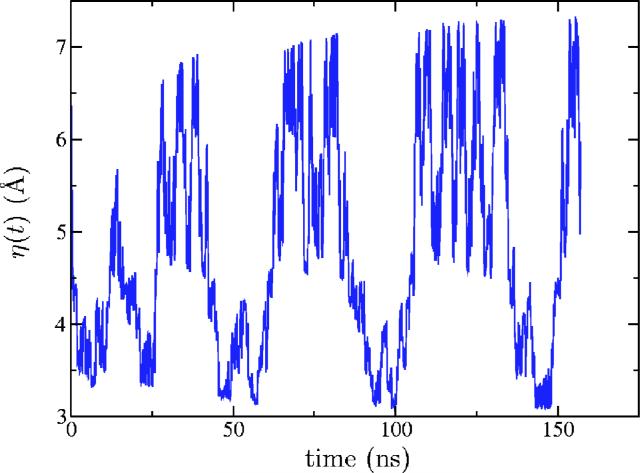
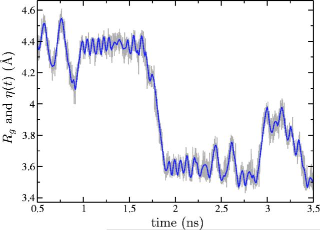
Second, we ran a metadynamics simulation until 5000 Gaussians were added to the hill potential, at which point the test particle had explored the entire range of interest (from a coil ensemble to linear conformations). The total time of the simulation was ≈157 ns. The trajectory of the test particle is presented in Fig. 3. Roughly speaking, values of η around 3–4 Å correspond to a random coil, around 4–5 Å to the β-hairpin conformation, and around 7 Å to the unfolded peptide. In Fig. 4 the time dependence of both R_g and the test particle position, η(t), is compared on a finer time scale. As expected for “good metadynamics,” R_g changes much faster than η(t)(which means that the chosen value of mass M is sufficient) and the value of R_g fluctuates around the value of η(t) (implying that the force constant K is also correctly chosen).

FIG. 3.

(Color online) The test particle trajectory in the metadynamics simulation of the Ace-(Gly)₂-Pro-(Gly)₃-Nme peptide.

FIG. 4.

(Color online) Time dependence (finer time scale) of the radius of gyration R_g (fast) and the test particle position η(t)(slow) in the metadynamics simulation of the Ace-(Gly)₂-Pro-(Gly)₃-Nme peptide.

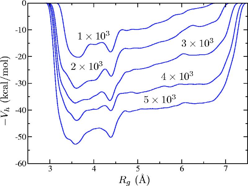
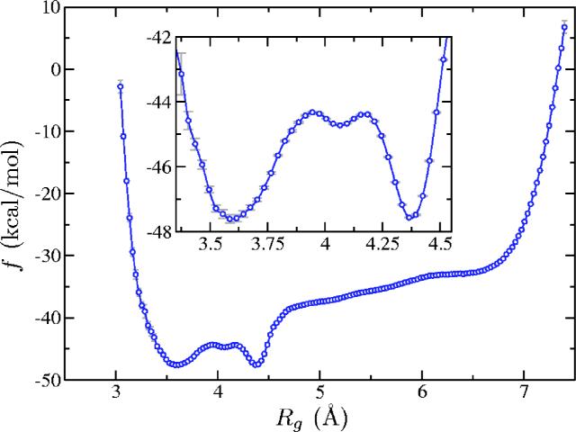
A few snapshots of the negated hill potential (the free energy) are shown in Fig. 5. Two minima were discovered in the metadynamics run: one at R_g≈3.6 Å that corresponds to a random coil conformation and another one at R_g≈4.4 Å that corresponds to β-hairpin conformation. These minima are separated by a broad barrier of approximately 4 kcal/mol.

FIG. 5.

(Color online) Snapshots of the negated hill potential (meant to approximate the free energy) [Eq. (2.5)] in the metadynamics simulation of the Ace-(Gly)₂-Pro-(Gly)₃-Nme peptide with 1 × 10³, 2 × 10³, 3 × 10³, 4 × 10³, and 5 × 10³ Gaussians.

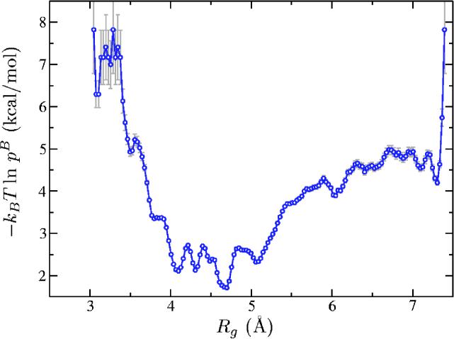
Third, we ran biased MD with the hill potential obtained with 5 × 10³ Gaussians for a total time of 5 × 10³ ns and computed the biased probability density as described in Sec. III. Having p^B(ξ) we computed the correction (Fig. 6) and corrected the free energy (Fig. 7). To estimate the statistical error of the probability density p^B(ξ) we used expression (26) from Ref. 43 assuming a 95% confidence interval. We note that the arguments leading to this expression assume uncorrelated samples. This might not be entirely the case for MD simulations. However, the total simulation time (5 × 10³ ns) was much greater than R_g's autocorrelation time (≈5 ns) and we found that the histogram has indeed “converged.”

FIG. 6.

(Color online) Umbrella correction [Eq. (2.8)] for the Ace-(Gly)₂-Pro-(Gly)₃-Nme peptide collected during a 5 × 10³ ns long biased molecular dynamics run.

FIG. 7.

(Color online) Corrected free energy for the Ace-(Gly)₂-Pro-(Gly)₃-Nme peptide (sum of the data from Figs. 5 and 6).

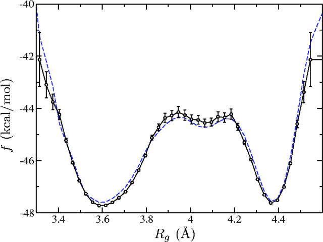
Finally, we ran REMD to get a reference free energy curve. The resulting free energy as a function of R_g is shown in Fig. 8. There is very good agreement between the two results. The main difference is that REMD does not visit “rare” (e.g., completely unfolded) states. In the present work, metadynamics alone (8 × 10⁷ MD steps) was approximately twice faster than REMD (16 × 10⁷ MD steps), but a meaningful comparison of the efficiency of the methods would require comparing both methods for the same range of R_g, using optimal parameters, which is beyond the scope of this work.

FIG. 8.

(Color online) Free energy for the Ace-(Gly)₂-Pro-(Gly)₃-Nme peptide as obtained from replica exchange molecular dynamics (solid) and from metadynamics with umbrella corrections (dashed). The statistical error is not shown for the latter.

B. Trialanine

In this section we discuss the free energy associated with the configurations of trialanine, both in implicit and explicit solvents, with the pair of dihedral angles (φ, ψ) chosen as the collective variable, as illustrated in Fig. 2.

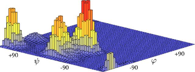
First, we ran regular MD for both implicit and explicit solvents for 40 ns. The histogram showing the probability distribution of the collective variable during the implicit solvent run is shown in Fig. 9. It can be seen that there are four maxima. A similar histogram is obtained for trialanine in explicit solvent: the main features (four maxima) persist, but their relative heights are slightly different.

FIG. 9.

(Color online) Histogram showing the equilibrium distribution of the collective variable (pair of dihedral angles shown in Fig. 2) for the trialanine molecule in implicit solvent (40 ns long molecular dynamics at T=300 K).

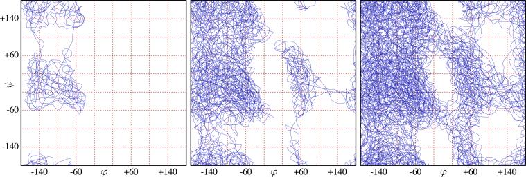
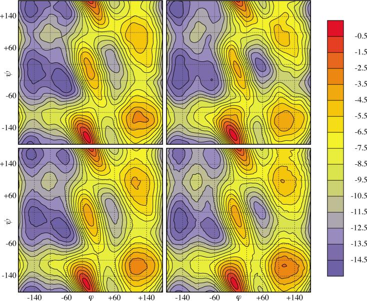
Second, we carry out metadynamics runs for both systems until 3 × 10⁴ Gaussians have been added to the hill potential. The total number of MD steps at that point corresponded to ≈12.5 ns in each case. The trajectory of the test particle for the implicit solvent simulation is presented in Fig. 10. As expected, the test particle explores regions of higher free energy after flooding the minima with hills. In particular, the left-handed α-helix local minimum, which is not accessible in regular MD at T=300 K, was discovered after a few thousands of Gaussians were added to the hill potential. With 3 × 10⁴ Gaussians the test particle trajectory has covered all $\mathbb{Q}$ in both implicit and explicit solvent systems. The negative of the hill potentials are shown in Fig. 11 (top row).

FIG. 10.

(Color online) Test particle trajectory for trialanine metadynamics simulation in implicit solvent after 1 × 10³ (left), 5 × 10³ (center), and 1 × 10⁴ (right) hills were accepted.

FIG. 11.

(Color) Free energies for zwitterionic trialanine (Fig. 2): as computed by metadynamics alone (top row), including umbrella corrections (bottom row). Left column: implicit solvent and right column: explicit solvent. In each case the free energy has been sampled on a 60×60 grid [bicubic interpolation (Ref. ⁴⁴) used]. The color changes from blue through yellow to red as the value of the free energy increases. The contour lines are plotted at −14.5, −13.5, . . . ,−0.5 kcal/mol.

Third, since the trajectories with 3 × 10⁴ Gaussians have covered all $\mathbb{Q}$, we took this last hill potential as biasing potential for biased molecular dynamics. For both implicit and explicit solvents we ran for 100 ns and recorded the values of the dihedral angles each 100 fs. The collective variable autocorrelation times were observed to be of the order of 1 and 100 ps for implicit and explicit solvent simulations, respectively, which is far smaller than the total simulation time. We computed histograms of the dihedral angles using 6° ×6° sized bins and corrected the free energies appropriately. For trialanine in explicit solvent, the maximum free energy correction was Δ_maxf=3.54 kcal/mol, with maximal statistical error of 0.73 kcal/mol (mean statistical error was 0.19 kcal/mol). For trialanine in implicit solvent, we obtained Δ_maxf=1.5 kcal/mol, with maximal statistical error of 0.25 kcal/mol (mean statistical error was 0.14 kcal/mol). We notice that umbrella sampling not only provides a very reliable error estimate (although, unfortunately, more costly) but also that this error is a function of the collective variable and can therefore be used to improve the accuracy of the free energy as obtained from metadynamics alone. The contour plots of the corrected free energies are shown in the bottom row in Fig. 11. Note that the free energies as obtained from metadynamics for implicit and explicit solvents (top row) differ considerably more than those incorporating the umbrella sampling corrections (bottom row). Differences in the latter are attributed to the treatment of the solvent.

V. CONCLUSIONS AND OUTLOOK

We have implemented the metadynamics method in the classical MD code AMBER 8 (Ref. ¹⁸) and used it to explore the free energy landscapes of two model peptides, Ace-(Gly)₂-Pro-(Gly)₃-Nme in vacuo and zwitterionic trialanine both in implicit and explicit solvent. Our main findings are as follows. Metadynamics (with corrections) can indeed give an excellent portrait of the free energy landscape of small peptides in the chosen collective variables. However, in spite of error estimates published in the literature, the metadynamics method still lacks a reliable free energy error estimate. To our best knowledge, these estimates only give the “reconstruction” accuracy, ignoring the “average” errors arising from finiteness of the mass and the spring constant. These last two quantities should in principle be as large as possible to ensure that the test particle moves slowly through the free energy landscape in order to accurately account for the entropy. A fairly good approximation of the free energy can be obtained by correcting the metadynamics run using biased molecular dynamics, but this can be potentially costly (REMD can be used to speed up the process). With respect to implementation, we have found that for classical simulations, the hill potential proposed by the original authors can be simplified without any loss of accuracy (the displacement-dependent Gaussians are not needed) and can be safely replaced by a sum of smoothly truncated Gaussians. Our form is better suited for rapid evaluation using the kd-tree data structure. We have also found that it is important to limit the speed of the test particle from above.

Metadynamics has had big success in systems with relatively few degrees of freedom, such as small molecules undergoing chemical reactions. The method is especially successful when it comes to evaluating very large energy barriers. As the number of degrees of freedom increases, the success of the method in mapping out a particular process depends to a considerable extent on insight in choosing the correct order parameter. Depending on the complexity of the problem, this may be quite challenging. In fairness, this problem is associated with all umbrella-type sampling methods. In addition, one has to concern oneself with the accurate evaluation of the entropic contributions, for which auxiliary methods may be required. With these caveats in mind, we believe that metadynamics is a sampling method that can be fruitfully applied to chemical and biomolecular simulations.

APPENDIX: POINT kD-TREE

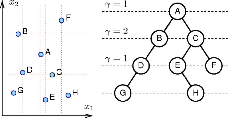
Point kd-tree³⁴ (k-dimensional tree) is a binary tree that can be used (among other things) to speedup orthogonal range queries over a set of points from a k-dimensional space ${\mathbb{R}}^k$. A kd-tree for a set of N points contains precisely N nodes. Each node stores a point's coordinates, a splitting dimension 1 ≤ γ≤k, and two pointers to its subtrees. In our work simple alternation is used for the splitting dimension: γ=1 +($\ell$ mod k), where $\ell$ denotes the node's level (a positive integer number which increases by 1 as one goes from parent node to its children). The tree is organized in such a way that the points from the left subtree of a node have γth coordinate, x_γ, less than γth coordinate of the parent node and the points from the right subtree have x_γ greater or equal to the parent's x_γ. The idea is illustrated in Fig. 12 for eight points from two-dimensional space. Further details, including insertion and neighbor lookup operations, can be found in numerous textbooks on data structures.

FIG. 12.

(Color online) An example kd-tree for eight points in two dimensions (k=2). The points were inserted in alphabetical order (for a different order the tree may have a different structure).

References

- 1.Weinan E, Vanden-Eijnden E. In: Lecture Notes in Computational Science and Engineering. Attinger S, Koumoutsakos P, editors. Springer; Berlin: 2004. [Google Scholar]
- 2.Darve E, Pohorille A. J. Chem. Phys. 2001;115:9169. [Google Scholar]
- 3.Sugita Y, Kitao A, Okamoto Y. J. Phys. Chem. 2000;113:6042. [Google Scholar]
- 4.Hansmann U. Chem. Phys. Lett. 1997;281:140. [Google Scholar]
- 5.Sugita Y, Okamoto Y. Chem. Phys. Lett. 1999;314:141. [Google Scholar]
- 6.Kumar S, Bouzida D, Swendsen RH, Kollman PA, Rosenberg J. J. Comput. Chem. 1992;13:1011. [Google Scholar]
- 7.Bartels C, Schaefer M, Karplus M. J. Chem. Phys. 1999;111:8048. [Google Scholar]
- 8.Mezei M. J. Comput. Phys. 1987;68:237. [Google Scholar]
- 9.Hooft RWW. J. Chem. Phys. 1992;97:6690. [Google Scholar]
- 10.Bartels C, Karplus M. J. Comput. Chem. 1997;18:1450. [Google Scholar]
- 11.Laio A, Parrinello M. Proc. Natl. Acad. Sci. U.S.A. 2002;99:12562. doi: 10.1073/pnas.202427399. [DOI] [PMC free article] [PubMed] [Google Scholar]
- 12.Iannuzzi M, Laio A, Parrinello M. Phys. Rev. Lett. 2003;90:238302. doi: 10.1103/PhysRevLett.90.238302. [DOI] [PubMed] [Google Scholar]
- 13.Car R, Parrinello M. Phys. Rev. Lett. 1985;55:2471. doi: 10.1103/PhysRevLett.55.2471. [DOI] [PubMed] [Google Scholar]
- 14.Andersen HC. J. Chem. Phys. 1980;72:2384. [Google Scholar]
- 15.Nose S. Mol. Phys. 1984;52:255. [Google Scholar]
- 16.Huber T, Torda AE, van Gunsteren WF. J. Comput.-Aided Mol. Des. 1994;8:695. doi: 10.1007/BF00124016. [DOI] [PubMed] [Google Scholar]
- 17.Hummer G, Kevrekidis I. J. Chem. Phys. 2003;118:10762. [Google Scholar]
- 18.Wang F, Landau DP. Phys. Rev. Lett. 2001;86:2050. doi: 10.1103/PhysRevLett.86.2050. [DOI] [PubMed] [Google Scholar]
- 19.Ensing B, Laio A, Gervasio FL, Parrinello M, Klein ML. J. Am. Chem. Soc. 2004;126:9492. doi: 10.1021/ja048285t. [DOI] [PubMed] [Google Scholar]
- 20.Churakov SV, Ianuzzi M, Parrinello M. J. Phys. Chem. B. 2004;108:11567. [Google Scholar]
- 21.Gervasio F, Laio A, Parrinello M. J. Am. Chem. Soc. 2005;124:2600. doi: 10.1021/ja0445950. [DOI] [PubMed] [Google Scholar]
- 22.Ceccarelli M, Danelon C, Laio A, Parrinello M. Biophys. J. 2004;87:58. doi: 10.1529/biophysj.103.037283. [DOI] [PMC free article] [PubMed] [Google Scholar]
- 23.Iannuzzi M, Parrinello M. Phys. Rev. Lett. 2004;93:025901. doi: 10.1103/PhysRevLett.93.025901. [DOI] [PubMed] [Google Scholar]
- 24.Stirling ALA, Ianuzzi M, Parrinello M. ChemPhysChem. 2004;5:1558. doi: 10.1002/cphc.200400063. [DOI] [PubMed] [Google Scholar]
- 25.Asciutto E, Sagui C. J. Phys. Chem. A. 2005;109:7682. doi: 10.1021/jp053428z. [DOI] [PubMed] [Google Scholar]
- 26.Lee JG, Asciutto E, Babin V, Sagui C, Darden TA, Roland C. J. Phys. Chem. B. 2006;110:2325. doi: 10.1021/jp055809i. [DOI] [PubMed] [Google Scholar]
- 27.Ikeda T, Hirata M, Kimura T. J. Chem. Phys. 2005;122:244507. doi: 10.1063/1.1940029. [DOI] [PubMed] [Google Scholar]
- 28.Case DA, Darden TA, Cheatham TE, III, et al. AMBER 8. University of California; San Francisco: 2004. [Google Scholar]
- 29.Gnanakaran S, Nymeyer H, Portman J, Sanbonmatsu KY, García AE. Curr. Opin. Struct. Biol. 2003;13:168. doi: 10.1016/s0959-440x(03)00040-x. [DOI] [PubMed] [Google Scholar]
- 30.García AE, Sanbonmatsu KY. Proteins. 2001;42:345. doi: 10.1002/1097-0134(20010215)42:3<345::aid-prot50>3.0.co;2-h. [DOI] [PubMed] [Google Scholar]
- 31.Zhou R, Berne B. Proc. Natl. Acad. Sci. U.S.A. 2001;96:14931. doi: 10.1073/pnas.201543998. [DOI] [PMC free article] [PubMed] [Google Scholar]
- 32.Chipot C, Hénin J. J. Chem. Phys. 2005;123:244906. doi: 10.1063/1.2138694. [DOI] [PubMed] [Google Scholar]
- 33.Weinan E, Vanden-Eijnden E. http://www.cims.nyu.edu/~eve2/metastable.pdf.
- 34.Bentley JL. Commun. ACM. 1975;18:509. [Google Scholar]
- 35.Ensing B, Laio A, Parrinello M, Klein M. J. Phys. Chem. B. 2005;109:6676. doi: 10.1021/jp045571i. [DOI] [PubMed] [Google Scholar]
- 36.Bussi G, Laio A, Parrinello M. Phys. Rev. Lett. 2006;96:090601. doi: 10.1103/PhysRevLett.96.090601. [DOI] [PubMed] [Google Scholar]
- 37.Bartels C, Karplus M. J. Phys. Chem. B. 1998;102:865. [Google Scholar]
- 38.Cornell WD, Cieplak P, Bayly CI, Gould IR, Merz KM, Ferguson DM, Spellmeyer DC, Fox T, Caldwell JW, Kollman PA. J. Am. Chem. Soc. 1995;117:5179. [Google Scholar]
- 39.Berendsen HJC, Postma JPM, van Gunsteren WF, Di Nola A, Haak JR. J. Chem. Phys. 1984;81:3684. [Google Scholar]
- 40.Darden TA, York DM, Pedersen LG. J. Chem. Phys. 1993;98:10089. [Google Scholar]
- 41.Essmann U, Perera L, Berkowitz ML, Darden T, Lee H, Pedersen LG. J. Chem. Phys. 1995;103:8577. [Google Scholar]
- 42.Jorgensen WL, Chandrasekhar J, Madura J, Klein ML. J. Chem. Phys. 1983;79:926. [Google Scholar]
- 43.Kobrak MN. J. Comput. Chem. 2003;24:1437. doi: 10.1002/jcc.10313. [DOI] [PubMed] [Google Scholar]
- 44.Preusser A. ACM Trans. Math. Softw. 1989;15:79. [Google Scholar]
- 45.This method is different from other adaptive umbrella sampling methods that use the potential energy, such as that introduced in Ref. 37. In that work, the authors use the potential energy as the collective variable, and successive biasing potentials are built using the probability distributions. This requires the partition of the energy collective variable into bins and the use of the WHAM and extrapolation techniques. The potential energy as collective variable has the advantage that it does not depend on the molecular geometry; however, due to practical reasons the range of potential energies that are sampled has to be restricted. The method can be costly since it requires many updates of the umbrella potential.