Generalization of the Gaussian electrostatic model: Extension to arbitrary angular momentum, distributed multipoles, and speedup with reciprocal space methods

Abstract

The simulation of biological systems by means of current empirical force fields presents shortcomings due to their lack of accuracy, especially in the description of the nonbonded terms. We have previously introduced a force field based on density fitting termed the Gaussian electrostatic model-0 (GEM-0) J.-P. Piquemal et al. [J. Chem. Phys. 124, 104101 (2006)] that improves the description of the nonbonded interactions. GEM-0 relies on density fitting methodology to reproduce each contribution of the constrained space orbital variation (CSOV) energy decomposition scheme, by expanding the electronic density of the molecule in s-type Gaussian functions centered at specific sites. In the present contribution we extend the Coulomb and exchange components of the force field to auxiliary basis sets of arbitrary angular momentum. Since the basis functions with higher angular momentum have directionality, a reference molecular frame (local frame) formalism is employed for the rotation of the fitted expansion coefficients. In all cases the intermolecular interaction energies are calculated by means of Hermite Gaussian functions using the McMurchie-Davidson [J. Comput. Phys. 26, 218 (1978)] recursion to calculate all the required integrals. Furthermore, the use of Hermite Gaussian functions allows a point multipole decomposition determination at each expansion site. Additionally, the issue of computational speed is investigated by reciprocal space based formalisms which include the particle mesh Ewald (PME) and fast Fourier-Poisson (FFP) methods. Frozen-core (Coulomb and exchange-repulsion) intermolecular interaction results for ten stationary points on the water dimer potential-energy surface, as well as a one-dimensional surface scan for the canonical water dimer, formamide, stacked benzene, and benzene water dimers, are presented. All results show reasonable agreement with the corresponding CSOV calculated reference contributions, around 0.1 and 0.15 kcal/mol error for Coulomb and exchange, respectively. Timing results for single Coulomb energy-force calculations for (H₂O)_n, n=64, 128, 256, 512, and 1024, in periodic boundary conditions with PME and FFP at two different rms force tolerances are also presented. For the small and intermediate auxiliaries, PME shows faster times than FFP at both accuracies and the advantage of PME widens at higher accuracy, while for the largest auxiliary, the opposite occurs.

I. INTRODUCTION

The simulation of biological systems at present relies mainly on the use of classical empirical force fields^1–5 due to their speed. In general these methods represent the nonbonded contributions by a collection of point charges for the Coulomb interaction and a 6−12 Van der Waals term that attempts to reproduce the exchange and dispersion contributions.⁶ A disadvantage of using simple isotropic atom-atom potentials is that this results in a loss of accuracy.⁷

More recently, methods based on distributed multipole expansions^7–10 have been proposed in order to improve the description of the electrostatic interaction.^11–13 However, the multipolar expansion fails to account for the charge penetration effects present at short range. This disadvantage has been addressed to an extent by the use of damping functions that correct the interaction energies at close intermolecular distances.^14–16

It has been shown that another possibility for the accurate determination of the intermolecular Coulomb contribution is by interacting the unperturbed frozen densities of the two molecules either numerically¹⁷ or analytically.¹⁸ The latter method is based on the density fitting (DF) formalism (Coulomb fitting),^19–21 where the electron density is expanded using Gaussian auxiliary basis sets (ABSs) centered on specific sites on the molecule. By employing the DF methodology, the intermolecular electrostatic contribution can be determined with any level of theory from which a one-electron relaxed density matrix can be obtained.

This formalism has been the foundation for the development of the Gaussian electrostatic model-0 (GEM-0).²² GEM-0 provides a total energy expression that separately reproduces each of the components of the interaction energy, namely, Coulomb, exchange repulsion, polarization, and charge transfer. It has been parametrized in order to reproduce reference constrained space orbital variation^23,24 (CSOV) values by using an ABS restricted to s-type functions (1=0). The exchange-repulsion contribution is computed by means of the overlap model proposed by Wheatley and Price,²⁵ and Domene et al.²⁶ while the polarization and charge transfer terms are calculated in the spirit of the sum of interactions between fragments ab initio^12,16 (SIBFA) scheme, using the electrostatic potentials and electric fields calculated with the fitted densities.

The choice of s-type Gaussian functions for the fitting procedure facilitates the rotation of the fitted densities of the rigid fragments, in addition to allowing a fast evaluation of the required integrals for the energy components. However, this requires the use of several extra fitting sites in order to achieve a good fit of the initial ab initio density. It was shown that the calculated expansion coefficients of the fitted density for a rigid molecule could be transferred to any fragment with the same internal geometry in a different orientation. Thus, the fitting procedure had to be performed only once for a single fragment of interest, thereby allowing the calculation of intermolecular interactions for any system once the fitting coefficients have been determined.

In order to demonstrate the applicability of the method, a water model with nine expansion sites was used to compute the total interaction energy and its individual components²² for several systems. Ten stationary points in the water dimer potential-energy surface (PES),^27,28 three water clusters, as well as two metal-water dimers were used as examples. Errors below thermal noise at room temperature (k_BT) were obtained for each component of the interaction energy.

In this contribution we present an extension of GEM-0 in order to include Gaussian ABSs of arbitrary angular momentum. We term this extension the Gaussian electrostatic model (GEM). The use of fitting basis with angular momentum greater than zero presents two issues that need to be addressed: numerical instabilities (noise) in the fitting procedure and rotation of the fitting coefficients. Noise in the fitting procedure is controlled by using a modified Tikhonov regularization method.²⁹ Additionally, a damped Coulomb kernel³⁰ for the fitting integrals is also employed for certain systems.

We have chosen to use Hermite Gaussian functions³¹ for the ABSs (Ref. ³²) to take advantage of the McMurchie-Davidson (MD) recursion for the Coulombic³³ and overlap³⁴ integrals. Hermite Gaussians, being defined by partial derivatives of a spherical Gaussian either with respect to local coordinates defined by a reference (local) site frame^8,13 or with respect to global coordinates, provide a straightforward solution to the transformation of the fitting coefficients by using the chain rule. Furthermore, we show that the use of Hermite Gaussians leads to a natural definition of distributed point multipoles centered on the fitting sites.

Additionally, we present three reciprocal space methods that are related to the Ewald compensation methods used in calculations for periodic systems.³⁵ Of these, the two fast Fourier transform (FFT) based methods enable efficient linear scaling calculation of intermolecular interactions using Hermite Gaussian functions.

In all cases the ABSs used in the calculations are composed of uncontracted Gaussians arranged in s and spd shells only as in Ref. 18. Shells of s functions correspond to Gaussians of angular momentum zero only. In the case of the spd shells, each Gaussian exponent is used to form 1s, 3p, and 5 (independent) d functions resulting in contributions only up to the quadrupole level for both the Hermite and multipole calculations. The calculations, however, generalize to arbitrary levels of angular momentum in a manner similar to Ref. 36.

We present intermolecular Coulomb interactions for the ten water dimers,^27,28 as well as one-dimensional (1D) electrostatic surface scans for a water dimer, a formamide dimer, a stacked benzene dimer, and a water-benzene dimer. Electronic densities at the B3LYP/6−31G* and B3LYP/aug-cc-pVTZ levels are fitted using four different ABSs. For the one-dimensional surface scans only densities at the B3LYP/6−31G* fitted with three ABSs are considered. Results for exchange repulsion at the same levels are also presented. All results are compared to reference values calculated with CSOV.^15,23 In addition, the Coulomb interaction energy for a set of water boxes of increasing size is calculated to predetermined accuracy using reciprocal space methods and timing results are discussed.

II. METHODS

In this section we present the theory and computational details employed in the present study. In Sec. II A we provide a brief explanation of the density fitting method and its implementation including the methods employed to control numerical instabilities. In Sec. II B we describe the transformation of the Cartesian Gaussian expansion coefficients to local Hermite coefficients, followed by the methodology to transform Hermite coefficients between coordinate frames in Sec. II C. Sec. II D presents the procedure to calculate site multipoles from local Hermite coefficients. Subsequently in Sec. II E the methods used to calculate the Coulomb and exchange-repulsion terms in the DF formalism are explained. The description of reciprocal space methods for computational speedup using Hermite Gaussians is presented in Sec. II F. Finally, in Sec. II G we describe the particular details of the calculations.

A. Density fitting

The use of ABSs for density fitting is a field of intense study. This method relies on the use of auxiliary basis functions to expand the molecular electron density. Briefly, the electron density may be fitted by minimizing the self-energy of the error in the density according to some metric $\widehat{O}$:^20,21,37,38

$$E_{\text{self}}=\langle \rho \left(r\right)-\stackrel{\sim }{\rho }\left(r\right)\mid \widehat{O}\mid \rho \left(r\right)-\stackrel{\sim }{\rho }\left(r\right)\rangle ,$$ (1)

where the approximate density $\stackrel{\sim }{\rho }\left(r\right)$ is expanded in an ABS based on Gaussian functions

$$\stackrel{\sim }{\rho }\left(r\right)=\sum _k{x}_{k}k\left(r\right).$$ (2)

The operator $\widehat{O}$ can take several forms, typically the Coulomb operator 1/r is employed.³⁰ The minimization of Eq. (1) (self-interaction error) with respect to the expansion coefficients x_l leads to a linear system of equations:

$$\frac{\partial E_{\text{self}}}{\partial x_l}=-2\sum _{\mu ,\nu }{P}_{\mu \nu }\langle \mu \nu \mid \widehat{O}\mid l\rangle +2\sum _k{x}_k\langle k\mid \widehat{O}\mid l\rangle ,$$ (3)

where P_μν is the density matrix. This equation may be used for the determination of the coefficients

$$\mathbf{x}={\mathbf{G}}^{-1}\mathbf{j},$$ (4)

where $\mathbf{j}=P_{\mu \nu }\langle \mu \nu \mid \widehat{O}\mid l\rangle$ and $\mathbf{G}=\langle k\mid \widehat{O}\mid l\rangle$.

Since G is symmetric and positive definite it may be diagonalized to obtain its inverse. In our previous studies we had employed a modification of the matrix inverse similar to a singular value decomposition (SVD) procedure²⁹ by setting the inverse of the eigenvalue to zero if it is below a certain cutoff. However, this method produces undesirable numerical instabilities (noise) when the number of basis functions starts to grow when using Gaussian functions as we and others have discussed previously.^18,39 In addition, we have observed that these instabilities are also present when using only s-type (spherical) functions²² albeit to a lower extent.

In the present implementation we have opted to use the Tikhonov regularization formalism,²⁹ similar to the constrained density fitting algorithm recently proposed by Misquitta and Stone.⁴⁰ In this method redundant basis set contributions are penalized by instead minimizing the following equation:

$$E_{\text{self}}+\lambda \sum _k{x}_k^2.$$ (5)

Additionally, Jung et al. have recently showed that the use of a damped Coulomb operator $\widehat{O}=\mathrm{erfc}\left(\beta r\right)∕r$ can be used for the fitting procedure.³⁰ These authors have employed this kernel to localize the integrals in order to increase the calculation speed of three center Coulomb integrals in a quantum mechanical program. For our purposes, the damped Coulomb operator may also be employed to attenuate the near singular behavior due to long range interactions present in G.

These expressions have been implemented by the authors in a FORTRAN90 code developed for the present study. All the required (real space) integrals are calculated using the McMurchie-Davidson recursions.³³ Besides implementing the noise control features explained above, this code generates the fitted coefficients in local frames for a Hermite basis and the corresponding site multipoles by means of the methods explained in the subsections below.

B. Hermite coefficients

One advantage of using fitted densities expressed in a linear combination of Gaussian functions is that the choice of Gaussian functions for the ABS need not be restricted to Cartesian Gaussians.³² In the present work we have chosen to use (normalized) Hermite Gaussian functions for the calculation of the intermolecular interactions:

$${\Lambda }_{tuv}(r,\alpha ,\mathbf{S})={\left(\frac{\alpha }{\pi }\right)}^{3∕2}{\left(\frac{\partial }{\partial S_x}\right)}^t{\left(\frac{\partial }{\partial S_y}\right)}^u{\left(\frac{\partial }{\partial S_z}\right)}^v\exp (-\alpha r_S^2),$$ (6)

where S denotes the expansion points.

The use of Hermite Gaussians in the calculation of the intermolecular interactions results in improved efficiency by the use of the MD recursions,³³ since the expensive Cartesian-Hermite transformation is avoided. Obtaining the Hermite expansion coefficients from the fitted Cartesian coefficients is straightforward since Hermite polynomials form a basis for the linear space of polynomials.⁴¹

Let hc_tuv and cc_tuv be the Hermite and Cartesian coefficients of order tuv, respectively, for an spd function with exponent α from the fitting basis. The zeroth order coefficient is

$$h{c}_{000}=c{c}_{000}+\frac{(c{c}_{200}+c{c}_{020}+c{c}_{002})}{2\alpha },$$ (7)

the first order coefficients (t+u+v=1) are

$$h{c}_{tuv}=-\frac{c{c}_{tuv}}{2\alpha },$$ (8)

and the second order coefficients (t+u+v=2) correspond to

$$h{c}_{tuv}=\frac{c{c}_{tuv}}{4{\alpha }^2}.$$ (9)

C. Coefficient transformations

As explained in Sec. I, in order to be able to use one set of fitting coefficients for the calculation of intermolecular interaction energies the coefficients must be transformed to each molecular fragment orientation. Additionally, the generalized Particle mesh Ewald (PME) approach outlined below requires that the coefficients be transformed to scaled fractional coordinates. The former transformation can be achieved by defining a global orthogonal coordinate system (global frame) and local orthogonal coordinate systems (local frame) for each fitting site in the fragment. Hermite Gaussians in the two coordinate systems, ${\Lambda }_{tuv}^g$ and ${\Lambda }_{tuv}^l$, can be simply related using the chain rule. The same approach works for the transformation to scaled fractional coordinates. This method has been previously developed for point dipoles and generalized to higher order multipoles.^36,42

For the local frames two reference axes are selected for each site, based on the geometry of the molecule. For instance, in Fig. 1, for the local frame on the oxygen atom the first axis (p₁=z) is along the bisector of the two hydrogen atoms, while the second axis (p₂=x) points to one of the hydrogen atoms. Once chosen, an orthogonal local frame represented by the orthogonal unit vectors x̂, ŷ, and ẑ can be defined as follows: $\widehat{z}={\mathbf{p}}_1∕\mid {\mathbf{p}}_1\mid ;\mathbf{u}={\mathbf{p}}_2-({\mathbf{p}}_2\cdot \widehat{z})$ and $\widehat{x}=\mathbf{u}∕\mid \mathbf{u}\mid ;\widehat{y}=\widehat{z}\times \widehat{x}$. This transformation has been explained in detail (as are the additional force terms on frame defining sites due to infinitesimal local frame rotations) in Refs. ³⁶ and ⁴². These frame definitions are similar to the definitions used in Ref. 7 and in the OPEP code.⁴³ Note that in the case of Hermite functions, the use of the chain rule to calculate the coefficient transformation matrix is straightforward since the 3×3 coordinate frame transformation matrices are constants.

FIG. 1.

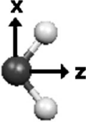
Local frame definition for the oxygen atom in water.

D. Site multipoles

In this subsection we present the methodology to obtain Cartesian point multipoles from the Hermite coefficients obtained in the fitting procedure. Note that since in the present work the highest order used for a Gaussian Hermite is 2 we will concentrate on multipoles expanded only up to quadrupole order. However, higher order multipoles can be obtained if an ABS with higher angular momentum is used, as explained below.

Challacombe et al. have shown that Hermite Gaussians have a simple relation to elements of the Cartesian multipole tensor.⁴⁴ Expanding on that work, once the Hermite coefficients have been determined, they may be employed to calculate point multipoles centered at the expansion sites. Thus, if hc_tuv represents the coefficient of a Hermite Gaussian of order Λ_tuv, then if this Hermite is normalized we have

$$h{c}_{000}\int {\Lambda }_{0}dr=h{c}_{000}.$$ (10)

This guarantees that higher order multipole integrals will integrate to integer numbers, for example, for the dipole integral in the x direction, d_x:

$$h{c}_{100}\int \int \int x{\Lambda }_{100}dxdydz=h{c}_{100}\int x\frac{\partial }{\partial S_x}{\Lambda }_{0}dx=-h{c}_{100}\int x\frac{\partial }{lx}{\Lambda }_{0}dx.$$ (11)

Integrating by parts this latter integral is evaluated as

$$-h{c}_{100}\int x{\Lambda }_{0}d{x}_{-\infty }^{\infty }+h{c}_{100}\int {\Lambda }_{0}dx=h{c}_{100}.$$ (12)

In the case of quadrupole integrals, ${\mathbf{Q}}_{x_a{x}_b}$, two cases need to be considered. When a=b, for example, for the x² quadrupole term, ${\mathbf{Q}}_{x^2}$,

$$\begin{array}{cc}\hfill h{c}_{200}\int \int \int x^2{\Lambda }_{200}dxdydz=& h{c}_{200}{x}^2\frac{\partial }{\partial x}{\phantom{\mid }{\Lambda }_0\mid }_{-\infty }^{\infty }\hfill \\ \hfill & -2h{c}_{200}\int x\frac{\partial }{\partial x}{\Lambda }_{0}dx\hfill \\ \hfill =& -2h{c}_{200}x{\phantom{\mid }{\Lambda }_0\mid }_{-\infty }^{\infty }\hfill \\ \hfill & +2h{c}_{200}\int {\Lambda }_{0}dx=2h{c}_{200}.\hfill \end{array}$$ (13)

When a ≠ b, for example, for the xy quadrupole term, Q_xy,

$$h{c}_{110}\int \int \int xy{\Lambda }_{110}dxdydz=h{c}_{110}x{\phantom{\mid }\frac{\partial }{\partial x}{\Lambda }_0\mid }_{-\infty }^{\infty }+h{c}_{110}y{\phantom{\mid }\frac{\partial }{\partial y}{\Lambda }_0\mid }_{-\infty }^y+h{c}_{110}\iint {\Lambda }_{0}dxdy=h{c}_{110}.$$ (14)

Note that in the case of the quadrupolar term when a=b there will be a contribution from the s-type Hermites, since this involves an even function; for example, for the x² quadrupole term

$$h{c}_{000}\int \int \int x^2{\Lambda }_{0}dxdydz=h{c}_{000}\int x^2{e}^{-\alpha x^2}dx=\frac{1}{2\alpha }h{c}_{000}.$$ (15)

However, this latter contribution is not present in the traceless point quadrupole expansion, nor does it contribute to the multipolar electrostatic interaction. The off-diagonal quadru-polar terms have no contribution from the zeroth order Hermites (nor do the dipolar terms) because the integral of an odd function is zero. In practice, following Stone's definition,⁷ we have used traceless quadrupoles.

Using the above distributed multipole definitions it is easy to calculate the penetration error in the site-site Coulomb interaction energy and to show that this error vanishes rapidly as the intersite distance increases. Thus density fitting, using a Hermite Gaussian ABS, leads to distributed multipoles that connect naturally with an accurate evaluation of the exact Coulomb interaction energy. This connection will be useful in the generation of damping functions¹⁵ to account for the penetration error when using these multipoles (work in progress). Recently we have demonstrated the superiority of fitted density compared to point charges or distributed multipoles in quantum mechanical/molecular mechanical (QM/MM) implementations.⁴⁵ Multipoles defined as above fit naturally into a multiscale treatment of the QM/MM problem, where the MM region nearest the active QM region is treated by density fitting using Hermite Gaussians, and more distant MM sites are treated by the corresponding multipoles together with their damping functions.

A further advantage of this approach to distributed multipoles is that, unlike some conventional multipole expansions,^46,47 the (spherical) multipole expansion obtained from Hermite Gaussians in this way is intrinsically finite of order t+u+v (i.e., the highest angular momentum in the ABS), similar to the multipoles obtained by Volkov and Coppens.⁴⁸ This is easily seen since Cartesian polynomials of order t+u+v can be expanded in a solid spherical harmonic expansion of the same and lower orders,⁷ leading to a similar expansion for the Hermite Gaussians:

$${\Lambda }_{tuv}=\left(\sum _{l=0}^{t+u+v}\sum _{m=-l}^l{D}_{tuv}^{lm}{r}^l{C}_{lm}(\theta ,\varphi )\right)\exp (-\alpha r_S^2).$$ (16)

Now, evaluating the spherical multipole contribution of Λ_tuv using Eq. (16) we obtain

$$\begin{array}{cc}\hfill Q_{l_2{m}_2}=& \int r^{l_2+2}dr\int {\Lambda }_{tuv}{C}_{l_2{m}_2}(\theta ,\varphi )\sin \theta d\theta d\phi \hfill \\ \hfill =& \sum _{l_1=0}^{t+u+v}\sum _{m_1=-l_1}^{l_1}\int D_{tuv}^{l_1{m}_1}{r}^{l_1}{r}^{l_2+2}\exp (-\alpha r^2)dr\hfill \\ \hfill & \times \int C_{l_1{m}_1}(\theta ,\phi )C_{l_2{m}_2}(\theta ,\phi )\sin \theta d\theta d\phi \hfill \\ \hfill =& \sum _{l_1=0}^{t+u+v}\sum _{m_1=-l_1}^{l_1}\int D_{tuv}^{l_1{m}_1}{r}^{l_1}{r}^{l_2+2}\exp (-\alpha r^2)dr{\delta }_{l_1{l}_2}{\delta }_{m_1{m}_2}\hfill \end{array}$$ (17)

and thus for $l_2>t+u+v,Q_{l_2{m}_2}=0$.

E. Frozen-core intermolecular interactions

Following the GEM-0 approach, the total intermolecular interaction energy can be computed as the sum of four intermolecular contributions:²⁴ Coulomb, exchange repulsion, polarization, and charge transfer. The first two are referred to as the frozen-core contribution while the latter are termed the induction term. In the present paper we will concentrate on the frozen core part exclusively.

In order to calculate the intermolecular Coulomb interaction between two molecules it is necessary to determine the nuclear-nuclear (N-N), nuclear-electron (N-e), and electron-electron (e-e) contributions to the Coulomb energy^49,50

$$E_{\text{Coulomb}}=E_{N\text{-}N}+E_{N\text{-}e}+E_{e\text{-}e}.$$ (18)

By making use of the approximate molecular electron density [Eq. (2)] we have previously shown¹⁸ that the intermolecular Coulomb energy can be calculated by

$$E_{\text{Coulomb}}=\sum _i\sum _j\frac{Z_{A_i}{Z}_{B_j}}{r_{A_i{B}_j}}+\sum _i\int \frac{Z_{A_i}{\stackrel{\sim }{\rho }}^B\left(r_2\right)}{r_{A_{i}2}}d{r}_2+\sum _j\int \frac{Z_{B_j}{\stackrel{\sim }{\rho }}^A\left(r_1\right)}{r_{1B_j}}d{r}_1+\iint \frac{{\stackrel{\sim }{\rho }}^A\left(r_1\right){\stackrel{\sim }{\rho }}^B\left(r_2\right)}{r_{12}}d{r}_{1}d{r}_2,$$ (19)

where $Z_{A_i}$ represents the nuclei on molecule A, ${\stackrel{\sim }{\rho }}^A$ represents the approximate density of molecule A, $Z_{B_j}$ represents the nuclei on molecule B, and ${\stackrel{\sim }{\rho }}^B$ represents the approximate density of molecule B. Note that in our force field formulation we use only the fitted density for the calculations, which differs from other DF methods used in DFT procedures where the fitted density is interacted with the density matrix. The use of only the fitted density (i.e., no density matrix) results in a less accurate representation.³⁹ However, this can be overcome by using extra points to place more ABSs such as at bond midpoints and/or lone pairs.^18,22

For the calculation of the exchange-repulsion contribution, we have used the overlap model initially proposed by Wheatley and Price,²⁵ which we have shown to be applicable using the DF formalism.²² This model relies on the observed proportionality between the overlap of the charge density and the exchange-repulsion energy

$$E_{\text{exchange-repulsion}}=K{\Omega }_{\rho },$$ (20)

where ${\Omega }_{\rho }$ is the overlap of charge density and K is a fitting parameter obtained as the slope of a linear regression of the overlap of charge density versus the corresponding ab initio exchange-repulsion energy values. By inserting the fitted densities of the interacting monomers into ${\Omega }_{\rho }$ we obtain

$${\Omega }_{\rho }=\int {\rho }^A\left(r_A\right){\rho }^B\left(r_B\right)dr\approx \int {\stackrel{\sim }{\rho }}^A\left(r_A\right){\stackrel{\sim }{\rho }}^B\left(r_B\right)dr.$$ (21)

F. Increasing computational efficiency using reciprocal space methods for Hermite Gaussians

In this section we describe the acceleration of the Coulomb and exchange-repulsion interaction calculations by using reciprocal space methods. For simplicity we first consider the overlap of charge density in an isolated cluster, describing how we split this into direct and reciprocal space contributions and then how each is calculated. Following this we discuss Coulomb interactions in an isolated cluster, using Ewald-type counterion and coion densities. Finally we discuss the extension of these results to a system under periodic boundary conditions (PBC).

To begin, consider a cluster of N identical molecules, e.g., water, each with an identical local frame density expansion over a set of expansion sites S. For this system the molecular density in the local frame can be expressed by

$${\stackrel{\sim }{\rho }}_{\mathrm{mol}}^l\left(\mathbf{r}\right)=\sum _{s\in \mathbf{S}}{\stackrel{\sim }{\rho }}_s^l\left(r\right)=\sum _{s\in \mathbf{S}}\sum _{\alpha \in A_s}{\stackrel{\sim }{\rho }}_{s,\alpha }^l\left(r\right)=\sum _{s\in \mathbf{S}}\sum _{\alpha \in A_s}\sum _{t,u,v}h{c}_{tuv}^l(\alpha ,s){\Lambda }_{tuv}^l(r,\alpha ,s),$$ (22)

where s∈S are the expansion points, A_s are the set of primitive Gaussian exponents on each expansion site, and $h{c}_{tuv}^l$ are the expansion coefficients in the local frame. Thus, the total density of the system in the global frame is

$${\stackrel{\sim }{\rho }}_{\mathrm{tot}}\left(r\right)=\sum _{n=1}^N\sum _{s\in {\mathbf{S}}_n}\sum _{\alpha \in A_{\mathbf{S}}}\sum _{t,u,v}h{c}_{tuv}^g(\alpha ,s){\Lambda }_{tuv}^g(r,\alpha ,s).$$ (23)

The overlap calculation, ${\Omega }_{\mathrm{tot}}=\int {\stackrel{\sim }{\rho }}_{\mathrm{tot}}\left(r\right){\stackrel{\sim }{\rho }}_{\mathrm{tot}}\left(r\right)d^{3}r$, can be accelerated by performing part of it in reciprocal space, using a method inspired by Fusti-Molnar and Pulay⁵¹ and Parrinello and co-workers.^52,53 For a given α₀ (called the splitting exponent) we can split ${\stackrel{\sim }{\rho }}_{\mathrm{tot}}$ into ${\stackrel{\sim }{\rho }}_{\mathrm{tot},c}$ and ${\stackrel{\sim }{\rho }}_{\mathrm{tot},d}$, where c and d denote compact and diffuse Hermite Gaussian functions, respectively.

$${\stackrel{\sim }{\rho }}_{\mathrm{tot},c}\left(r\right)=\sum _{n=1}^N\sum _{s\in {\mathbf{S}}_n}\sum _{\alpha \in A_{\mathbf{S}};\alpha \ge {\alpha }_0}\sum _{t,u,v}h{c}_{tuv}^g(\alpha ,s){\Lambda }_{tuv}^g(r,\alpha ,s),$$ (24)

$${\stackrel{\sim }{\rho }}_{\mathrm{tot},d}\left(r\right)=\sum _{n=1}^N\sum _{s\in {\mathbf{S}}_n}\sum _{\alpha \in A_{\mathbf{S}};\alpha <{\alpha }_0}\sum _{t,u,v}h{c}_{tuv}^g(\alpha ,s){\Lambda }_{tuv}^g(r,\alpha ,s).$$ (25)

Using this definition the total overlap becomes

$${\Omega }_{\mathrm{tot}}={\int }_{R^3}{\stackrel{\sim }{\rho }}_{\mathrm{tot},c}\left(r\right){\stackrel{\sim }{\rho }}_{\mathrm{tot},c}\left(r\right)dr+2{\int }_{R^3}{\stackrel{\sim }{\rho }}_{\mathrm{tot},c}\left(r\right){\stackrel{\sim }{\rho }}_{\mathrm{tot},d}\left(r\right)dr+{\int }_{R^3}{\stackrel{\sim }{\rho }}_{\mathrm{tot},d}\left(r\right){\stackrel{\sim }{\rho }}_{\mathrm{tot},d}\left(r\right)dr,$$ (26)

where the first integral is calculated in direct space and the latter two will be reexpressed in order to calculate them in reciprocal space. Note that the reciprocal contribution to the intramolecular (self) overlap needs to be calculated in direct space and subtracted when using this method. To employ reciprocal space methods the density of the cluster needs to be extended periodically. To this end, for any tolerance δ we can define an effective radius R_δ of the cluster with

$${\int }_{r>R_{\delta }}{\stackrel{\sim }{\rho }}_{\mathrm{tot}}\left(r\right)dr<\delta .$$ (27)

Let T>2R_δ, and for any site s∈S_n and any α, t, u, and v, define the periodic extension of ${\Lambda }_{tuv}^g$ by

$${\Lambda }_{tuv}^{g,P}(r,\alpha ,s)=\sum _{l_1}\sum _{l_2}\sum _{l_3}{\Lambda }_{tuv}^g(r+T(l_1,l_2,l_3),\alpha ,s).$$ (28)

Note that ${\Lambda }_{tuv}^{g,P}$ is periodic with period T. Define the periodic extension of ${\stackrel{\sim }{\rho }}_{\mathrm{tot},c}$ and ${\stackrel{\sim }{\rho }}_{\mathrm{tot},d}$ using ${\Lambda }_{tuv}^{g,P}$ and expressions similar to Eqs. (24) and (25). Then using these periodic extensions and Parseval's relations⁵⁴ we can approximate Ω_tot as

$$\begin{array}{cc}\hfill {\Omega }_{\mathrm{tot}}\approx & {\int }_{R^3}{\stackrel{\sim }{\rho }}_{\mathrm{tot},c}\left(r\right){\stackrel{\sim }{\rho }}_{\mathrm{tot},c}\left(r\right)dr+2{\int }_{{\mathcal{T}}^3}{\stackrel{\sim }{\rho }}_{\mathrm{tot},c}^P\left(r\right){\stackrel{\sim }{\rho }}_{\mathrm{tot},d}^P\left(r\right)dr\hfill \\ \hfill & +{\int }_{{\mathcal{T}}^3}{\stackrel{\sim }{\rho }}_{\mathrm{tot},d}^P\left(r\right)\rho \left(r\right){\stackrel{\sim }{\rho }}_{\mathrm{tot},d}^P\left(r\right)dr\hfill \\ \hfill =& {\int }_{R^3}{\stackrel{\sim }{\rho }}_{\mathrm{tot},c}\left(r\right){\stackrel{\sim }{\rho }}_{\mathrm{tot},c}\left(r\right)dr+T^3\sum _{\mathbf{m}}{\widehat{\stackrel{\sim }{\rho }}}_{\mathrm{tot},c}^P\left(\mathbf{m}\right){\widehat{\stackrel{\sim }{\rho }}}_{\mathrm{tot},d}^P(-\mathbf{m})\hfill \\ \hfill & +T^3\sum _{\mathbf{m}}{\widehat{\stackrel{\sim }{\rho }}}_{\mathrm{tot},c}^P(-\mathbf{m}){\widehat{\stackrel{\sim }{\rho }}}_{\mathrm{tot},d}^P\left(\mathbf{m}\right)+T^3\sum _{\mathbf{m}}{\widehat{\stackrel{\sim }{\rho }}}_{\mathrm{tot},d}^P\left(\mathbf{m}\right){\widehat{\stackrel{\sim }{\rho }}}_{\mathrm{tot},d}^P(-\mathbf{m}),\hfill \end{array}$$ (29)

where ${\mathcal{T}}^3$ denotes the cube of side T centered at the origin, m=(m₁ ,m₂ ,m₃)/T, and ${\widehat{\stackrel{\sim }{\rho }}}_{\mathrm{tot},c}^P$ (m) is given by

$${\widehat{\stackrel{\sim }{\rho }}}_{\mathrm{tot},c}^P\left(\mathbf{m}\right)=\frac{1}{T^3}{\int }_{{\mathcal{T}}^3}{\stackrel{\sim }{\rho }}_{\mathrm{tot},c}^P\left(r\right)\exp (-2\pi i\mathbf{m}\cdot r)d^{3}r=\frac{1}{T^3}{\int }_{R^3}{\stackrel{\sim }{\rho }}_{\mathrm{tot},c}\left(r\right)\exp (-2\pi i\mathbf{m}\cdot r)d^{3}r,$$ (30)

and ${\widehat{\stackrel{\sim }{\rho }}}_{\mathrm{tot},d}^P$ (m) is defined similarly.

Thus, recalling Eq. (23), Ω reduces to the efficient real space evaluation of the overlap of compact Hermite Gaussian functions and the efficient approximation of the Fourier coefficients of compact and diffuse Hermite Gaussian functions.

1. Direct space integrals

The first integral on the right hand side (RHS) of Eq. (29) is calculated in direct space. For the direct space evaluation we use the MD recursion³³ as explained above. The MD recursion was developed to evaluate Coulombic integrals and later extended to treat overlap.³⁴ To keep the paper self-contained we prove a more general version of this recursion, applicable to Cartesian derivatives of any smooth function of r.

For any function $f\left(r\right),r={(x^2+y^2+z^2)}^{1∕2}$ we want an efficient recursion for the derivatives ${(\partial ∕\partial x)}^t{(\partial ∕\partial y)}^u{(\partial ∕\partial z)}^{v}f\left(r\right)$. Following the notation in the original MD paper, let R(0,0,0,0)= f(r), R(0,0,0,n+1)=1/r(∂ /∂r)R(0,0,0,n), and $R(t,u,v,n)={(\partial ∕\partial x)}^t{(\partial ∕\partial y)}^u{(\partial ∕\partial z)}^{v}R(0,0,0,n)$. In particular, ${(\partial ∕\partial x)}^t{(\partial ∕\partial y)}^u{(\partial ∕\partial z)}^{v}f\left(r\right)=R(t,u,v,0)$. Then

$$\begin{array}{cc}\hfill & R(t+1,u,v,n)=xR(t,u,v,n+1)+tR(t-1,u,v,n+1),\hfill \\ \hfill & R(t,u,+1,v,n)=yR(t,u,v,n+1)+uR(t,u-1,v,n+1),\hfill \\ \hfill & R(t,u,v+1,n)=zR(t,u,v,n+1)+vR(t,u,v-1,n+1).\hfill \end{array}$$ (31)

This can be proven as follows:

$$\begin{array}{cc}\hfill R(t+1,u,v,n)& ={\left(\frac{\partial }{\partial x}\right)}^{t+1}{\left(\frac{\partial }{\partial y}\right)}^u{\left(\frac{\partial }{\partial z}\right)}^{v}R(0,0,0,n)\hfill \\ \hfill & ={\left(\frac{\partial }{\partial y}\right)}^u{\left(\frac{\partial }{\partial z}\right)}^v{\left(\frac{\partial }{\partial x}\right)}^t\left(\frac{\partial }{\partial x}\right)R(0,0,0,n)\hfill \\ \hfill & ={\left(\frac{\partial }{\partial y}\right)}^u{\left(\frac{\partial }{\partial z}\right)}^v{\left(\frac{\partial }{\partial x}\right)}^t\left(\frac{\partial }{\partial r}\right)R(0,0,0,n)\frac{\partial r}{\partial x}\hfill \\ \hfill & ={\left(\frac{\partial }{\partial y}\right)}^u{\left(\frac{\partial }{\partial z}\right)}^v{\left(\frac{\partial }{\partial x}\right)}^t\left(\frac{\partial }{\partial r}\right)\frac{x}{r}\left(\frac{\partial }{\partial r}\right)R(0,0,0,n)\hfill \\ \hfill & ={\left(\frac{\partial }{\partial y}\right)}^u{\left(\frac{\partial }{\partial z}\right)}^v{\left(\frac{\partial }{\partial x}\right)}^{t}xR(0,0,0,n+1).\hfill \end{array}$$ (32)

Using Leibniz' rule on the last line of Eq. (32) we obtain Eq. (31). The recursions for R(t,u+1,v,n) and R(t,u,v+1,n) are obtained similarly. The use of this method allows the determination of all the direct space integrals used in this study, i.e., overlap, Coulomb, and damped Coulomb, for each of which the required starting function f(r) is known. Ahlrichs has recently shown that a similar generalization can be obtained for the Obara-Saika recursion.⁵⁵

2. Reciprocal space integrals

In order to evaluate the two sums on the RHS of Eq. (29) we need to obtain the Fourier coefficients of ${\stackrel{\sim }{\rho }}_{\mathrm{tot},c}^P\left(\mathbf{m}\right)$ and ${\stackrel{\sim }{\rho }}_{\mathrm{tot},d}^P\left(\mathbf{m}\right)$. Note that these need to be calculated separately to avoid redundant calculation of the compact-compact interactions, which in any case do not converge for reasonable grid sizes.

The first procedure to obtain these coefficients is the explicit evaluation of the Fourier transform:

$${\widehat{\Lambda }}_{tuv}^{g,P}(\mathbf{m},\alpha ,s)=\frac{1}{T^3}{\left(\frac{\alpha }{\pi }\right)}^{3∕2}{\left(\frac{\partial }{\partial s_x}\right)}^t{\left(\frac{\partial }{\partial s_y}\right)}^u{\left(\frac{\partial }{\partial s_z}\right)}^v\times \exp \left(-\frac{{\pi }^2{\mathbf{m}}^2}{\alpha }\right)\exp (-2\pi i\mathbf{m}\cdot s).$$ (33)

Then ${\widehat{\stackrel{\sim }{\rho }}}_{\mathrm{tot}}^P\left(\mathbf{m}\right)$ can be obtained by linear combination of ${\widehat{\Lambda }}_{tuv}^{g,P}(\mathbf{m},\alpha ,s)$. Note that in general the number of reciprocal vectors m needed in Eq. (29) to converge the sums to a given tolerance scales linearly with the number of molecules N.⁷³ Since the number of basis elements ${\Lambda }_{tuv}^{g,P}$ also scales linearly with N, this method scales as order N² as in regular Ewald summation. One way to avoid the O(N²) scaling is to employ FFTs, which reduce the scaling to N log N. Two methods that employ FFT's have been implemented as explained below.

The second method we have implemented for the determination of the Fourier coefficients is the PME method. The use of PME is accomplished by rewriting the complex exponential as

$$\exp (-2\pi i\mathbf{m}\cdot s)=\exp \left(-2\pi i\frac{m_1}{M}{u}_1\right)\exp \left(-2\pi i\frac{m_2}{M}{u}_2\right)\times \exp \left(-2\pi i\frac{m_3}{M}{u}_3\right),$$ (34)

where, e.g., $u_1=M(s_x∕T)$ and T/M is the grid step size (in a. u.) of the PME grid. Next we approximate $\exp (-2\pi i(m_1∕M)u_1)$ by the Euler spline $g_q(m_1∕M,u_1)$ as defined by Essmann et al.⁵⁶ and optimized by Toukmaji et al.⁴² Using this definition for the complex exponential we obtain

$${\widehat{\Lambda }}_{tuv}^{g,P}{(\mathbf{m},\alpha ,s)}_{\mathrm{PME}}=\frac{1}{T^3}{\left(\frac{\alpha }{\pi }\right)}^{3∕2}\exp \left(-\frac{{\pi }^2{\mathbf{m}}^2}{\alpha }\right)\times {\left(\frac{\partial }{\partial s_x}\right)}^t{\left(\frac{\partial }{\partial s_y}\right)}^u{\left(\frac{\partial }{\partial s_z}\right)}^v{g}_q\left(u_1\right)g_q\left(u_2\right)g_q\left(u_3\right).$$ (35)

The partial derivatives with respect to Cartesian coordinates can be reexpressed in terms of ∂ /∂u₁,∂ /∂u₂,∂ /∂u₃ and the coefficients of the Hermites transformed to the (u₁,u₂,u₃) coordinate system. Methods for the efficient evaluation of these approximations have been explained in detail by Sagui et al.³⁶ Note that separate grids are needed for each exponent on the ABS, except when it only contains s-type functions with constant coefficients.

The third method is to directly sample the density on the grid as in the fast Fourier-Poisson (FFP) method of York and Yang⁵⁷ or the very similar Fourier transform Coulomb (FTC) method by Fusti-Molnar and Pulay.⁵¹ In this case ${\stackrel{\sim }{\rho }}_{\mathrm{tot},c}^P$ cannot be directly sampled, as discussed by Fusti-Molnar and Pulay. These authors solved this problem by using a modified low-pass filter operation on the compact basis elements. We have instead chosen to use a Gaussian splitting method inspired by Shan et al.⁵⁸ to render the core Hermite Gaussians more diffuse and the diffuse more compact.

Specifically, consider an individual term ${\Lambda }_{tuv}^{g,P}(\mathbf{m},{\alpha }_c,s_1){\Lambda }_{t^{\prime }{u}^{\prime }{v}^{\prime }}^{g,P}(\mathbf{m},{\alpha }_d,s_2)$ from the second sum of Eq. (29), where α_c≥α₀ and α_d<α₀.

For any $\stackrel{‒}{\alpha }>{\alpha }_0$ replace α_c by ${\alpha }_c^{\prime }={\alpha }_c\stackrel{‒}{\alpha }∕(\stackrel{‒}{\alpha }+{\alpha }_c)$ and α_d by ${\alpha }_d^{″}={\alpha }_d\stackrel{‒}{\alpha }∕(\stackrel{‒}{\alpha }-{\alpha }_d)$. In practice we have found that a good choice is $\stackrel{‒}{\alpha }=2{\alpha }_0$ because in this case ${\alpha }_c^{\prime }$ and ${\alpha }_d^{″}$ all tend to cluster near $\stackrel{‒}{\alpha }$ so that a uniform grid for sampling can be chosen. Then we note that

$${\widehat{\Lambda }}_{tuv}^{g,P}(\mathbf{m},{\alpha }_c,s_1){\widehat{\Lambda }}_{t^{\prime }{u}^{\prime }{v}^{\prime }}^{g,P}(-\mathbf{m},{\alpha }_d,s_2)={\widehat{\Lambda }}_{tuv}^{g,P}(\mathbf{m},{\alpha }_c^{\prime },s_1){\widehat{\Lambda }}_{t^{\prime }{u}^{\prime }{v}^{\prime }}^{g,P}(-\mathbf{m},{\alpha }_d^{″},s_2),$$ (36)

where ${\Lambda }_{tuv}^{g,P}(r,{\alpha }_c^{\prime },s_1)$ and ${\Lambda }_{t^{\prime }{u}^{\prime }{v}^{\prime }}^{g,P}(r,{\alpha }_d^{″},s_2)$ can be directly sampled.

In the case of diffuse-diffuse interactions

$${\widehat{\Lambda }}_{tuv}^{g,P}(\mathbf{m},{\alpha }_{d_1},s_1){\widehat{\Lambda }}_{t^{\prime }{u}^{\prime }{v}^{\prime }}^{g,P}(-\mathbf{m},{\alpha }_{d_2},s_2)={\widehat{\Lambda }}_{tuv}^{g,P}(\mathbf{m},{\alpha }_{d_1}^{″},s_1){\widehat{\Lambda }}_{t^{\prime }{u}^{\prime }{v}^{\prime }}^{g,P}(-\mathbf{m},{\alpha }_{d_2}^{″},s_2)\exp \left(\frac{-2{\pi }^2{\mathbf{m}}^2}{\stackrel{‒}{\alpha }}\right),$$ (37)

thus, the diffuse-diffuse interactions are corrected in reciprocal space by the factor exp $(-2\pi {\mathrm{m}}^2∕\stackrel{‒}{\alpha })$.

Note that in general the calculation of the exchange interaction requires different proportionality constants K for each molecular pair, thus different grids for different molecules. Nevertheless, these reciprocal space methods can be useful if most of the molecules are of one or two types such as a solute in a solvent bath. In the systems we have tested so far we have seen only modest reduction in computing time (see below). However, for systems with diffuse functions (thus, many direct space interactions), we expect greater savings by the use of these reciprocal space methods.

3. Coulomb interaction with Ewald splitting

To extend the above reciprocal space methods to Coulomb interactions in an isolated cluster we use the truncated Coulomb kernel g_δ(r) defined by g_δ(r)=1/r,r≤2R_δ and g_δ(r)=0,r>2R_δ following Fusti-Molnar and Pulay.⁵¹ In addition we now choose T twice as large as in the overlap case, i.e., satisfying T>4R_δ so that periodic images of the cluster do not interact via g_δ(r). Finally we introduce counter- and co-ion densities³⁵ (Ewald splitting method) to allow efficient cutoffs in the direct space compact-compact interactions. Here we discuss the e-e Coulombic integrals (N-e and N-N terms are handled similarly). Recalling that compact and diffuse Hermites are defined in terms of the exponent α₀, the site density is reexpressed as

$${\stackrel{\sim }{\rho }}_s^g\left(r\right)={\stackrel{\sim }{\rho }}_{s,c}^g\left(r\right)+{\stackrel{\sim }{\rho }}_{s,d}^g\left(r\right)=({\stackrel{\sim }{\rho }}_{s,c}^g\left(r\right)-{\stackrel{\sim }{\rho }}_{s,{\alpha }_0}^g\left(r\right))+({\stackrel{\sim }{\rho }}_{s,{\alpha }_0}^g\left(r\right)+{\stackrel{\sim }{\rho }}_{s,d}^g\left(r\right)),$$ (38)

where

$${\stackrel{\sim }{\rho }}_{s,{\alpha }_0}^g\left(r\right)=\sum _{tuv}\left(\sum _{a\in A_{\mathbf{S}};\alpha \ge {\alpha }_0}h{c}_{tuv}^g(\alpha ,s)\right){\Lambda }_{tuv}^g({\alpha }_0,s).$$ (39)

By using this splitting scheme, $\langle {\stackrel{\sim }{\rho }}_{s_1,c}^g\left(r\right)-{\stackrel{\sim }{\rho }}_{s_1,{\alpha }_0}^g\left(r\right)\parallel {\stackrel{\sim }{\rho }}_{s_2,c}^g\left(r\right)-{\stackrel{\sim }{\rho }}_{s_2,{\alpha }_0}^g\left(r\right)\rangle$ can be neglected if |s₁−s₂| exceeds twice the Gaussian extent of ${\stackrel{\sim }{\rho }}_{s,{\alpha }_0}^g\left(r\right)$ since ${\stackrel{\sim }{\rho }}_{s,c}^g\left(r\right)-{\stackrel{\sim }{\rho }}_{s,{\alpha }_0}^g\left(r\right)$ has no nonzero multipole moments.³¹

The compact-diffuse and diffuse-diffuse integrals in reciprocal space are treated similarly to the overlap case by using Parseval's relations, the fact that the convolution of g_δ(r) with a periodic density is itself periodic, the convolution product relation in reciprocal space,⁵⁴ and the Fourier transform of g_δ(r) to obtain, e.g.,

$$\begin{array}{c}{\int }_{R^3}{\int }_{R_3}\frac{{\stackrel{\sim }{\rho }}_{\mathrm{tot},d}\left(r_1\right){\stackrel{\sim }{\rho }}_{\mathrm{tot},d}\left(r_2\right)}{\mid r_1-r_2\mid }d{r}_{1}d{r}_2\\ \approx {\int }_{{\mathcal{T}}^3}{\int }_{{\mathcal{T}}^3}{\stackrel{\sim }{\rho }}_{\mathrm{tot},d}^P\left(r_1\right)g_{\delta }(r_2-r_1){\stackrel{\sim }{\rho }}_{\mathrm{tot},d}^P\left(r_2\right)d{r}_1,d{r}_2\\ =T^3\sum _{\mathbf{m}}{\widehat{\stackrel{\sim }{\rho }}}_{\mathrm{tot},d}^P\left(\mathbf{m}\right){\widehat{\stackrel{\sim }{\rho }}}_{\mathrm{tot},d}^P(-\mathbf{m})\frac{1-\cos \left(4\pi \mid \mathbf{m}\mid R_{\delta }\right)}{\pi {\mathbf{m}}^2},\end{array}$$ (40)

where |m| denotes the norm of the vector m=(m₁,m₂,m₃).

The compact-compact integrals in real space can be further accelerated by

$$\begin{array}{cc}\hfill & \langle {\stackrel{\sim }{\rho }}_{s_1,c}^g\left(r\right)-{\stackrel{\sim }{\rho }}_{s_1,{\alpha }_0}^g\left(r\right)\parallel {\stackrel{\sim }{\rho }}_{s_2,c}^g\left(r\right)-{\stackrel{\sim }{\rho }}_{s_2,{\alpha }_0}^g\left(r\right)\rangle \hfill \\ \hfill & =\sum _{{\alpha }^{\prime }\in A_{s_2};{\alpha }^{\prime }\ge {\alpha }_0}\sum _{\alpha \in A_{s_1};\alpha \ge {\alpha }_0}\langle {\stackrel{\sim }{\rho }}_{s_1,\alpha }^g\left(r\right)\parallel {\stackrel{\sim }{\rho }}_{s_2,{\alpha }^{\prime }}^g\left(r\right)-{\delta }_{s_2,{\alpha }^{\prime }}\rangle \hfill \\ \hfill & -\sum _{{\alpha }^{\prime }\in A_{s_2};{\alpha }^{\prime }\ge {\alpha }_0}\langle {\stackrel{\sim }{\rho }}_{s_1,{\alpha }_0}^g\left(r\right)\parallel {\stackrel{\sim }{\rho }}_{s_2,{\alpha }^{\prime }}^g\left(r\right)-{\delta }_{s_2,{\alpha }^{\prime }}\rangle \hfill \\ \hfill & -\sum _{\alpha \in A_{s_1};\alpha \ge {\alpha }_0}\langle {\stackrel{\sim }{\rho }}_{s_1,\alpha }^g\left(r\right)\parallel {\stackrel{\sim }{\rho }}_{s_2,{\alpha }_0}^g\left(r\right)-{\delta }_{s_2},{\alpha }_0\rangle +\langle {\stackrel{\sim }{\rho }}_{s_1,{\alpha }_0}^g\left(r\right)\mid \hfill \\ \hfill & \times \mid {\stackrel{\sim }{\rho }}_{s_2,{\alpha }_0}^g\left(r\right)-{\delta }_{s_2,{\alpha }_0}\rangle ,\hfill \end{array}$$ (41)

where for any α,

$${\delta }_{s_2,\alpha }=\sum _{tuv}h{c}_{tuv}^g(\alpha ,s_2){\Lambda }_{tuv}(r,{\alpha }_{\infty },s_2),$$ (42)

and α_∞ corresponds to a very large exponent (effectively replacing the Hermite with exponent α by its multipole approximation). Thus as above, the individual terms on the right hand side of Eq. (41) can be neglected as soon as s₁+s₂ is larger than the sum of the relevant Gaussian extents.³¹

4. Extension to periodic boundary conditions

In the case of a periodic system with unit cell U (triclinic in general) the fitted density is already periodic and can be split as above into compact and diffuse components. The overlap and Coulomb integrals extend over U by definition and Parseval's relations hold for the compact-diffuse and diffuse-diffuse interactions. The overlap calculation converges in direct space using cutoff methods but as with the cluster calculation is accelerated considerably by reciprocal space methods.

The Coulomb interaction converges slowly in direct space, if the unit cell is neutral, and the result is conditional on summation order. For point charges the Ewald sum can be interpreted (in the limit) as the Coulomb energy of the unit cell embedded in a large array of periodic copies of itself, which is further embedded in a conducting medium,⁵⁹ and this interpretation holds as well for the present case of nuclei plus fitted electron density. The same Ewald splitting strategy is used as described above for finite clusters with g_δ(r) replaced by 1/r; however, in contrast to that case, under PBC the system must be neutral, due to the infinite range of the non-truncated Coulomb interaction. In practice, each of the compact and diffuse contributions is neutralized by a uniform plasma. With reciprocal space methods and overall net-neutral systems this is achieved automatically by the neglect of the m=0 term. If real space methods such as multigrid⁶⁰ are used instead to solve Poisson's equation, the grid must be explicitly neutralized.

G. Computational details

Relaxed one-electron molecular densities for the test cases were obtained from ab initio calculations performed with CADPAC.⁶¹ For the determinations of the ten water dimers, the electronic densities were calculated at the B3LYP (Refs. ⁶² and ⁶³) levels with the 6−31G* and aug-cc-pVTZ basis sets. Electronic densities for all molecules in the 1D surface scans were obtained at the B3LYP/6−31G* level only. The geometries for the ten water dimers were based on the geometries reported by van Duijneveldt–van de Rijdt et al..²⁸ All molecular geometries were optimized at the B3LYP/aug-cc-pVTZ level. Reference values for all systems were calculated at the corresponding levels of theory and basis set with the CSOV method,^23,24 using the same molecular geometries. For the CSOV electrostatic and exchange-repulsion analysis, all calculations were performed with a modified version of the HONDO95 package.^24,50

The density fit was done with three different ABSs. The first two correspond to DGAUSS A1 and P1 Coulomb fitting ABS.^64,65 The final ABS, denoted g03, was obtained from the automatic fitting utility from GAUSSIAN03.⁶⁶ The g03 ABS was obtained by using the 6−311G** basis sets for the corresponding atoms.¹⁸ Due to the extensive size of this last ABS, the f function orbitals were deleted and only the s and spd functions were retained. In the case of the P1 set, the original basis sets contain only s and d basis functions; in this study the d functions were expanded to represent spd shells.^64,65 Additional calculations with the CFIT basis set⁶⁷ for the ten water dimers were performed, using the same “transformation” as for the g03 ABS. ABSs were placed on all atomic positions, as well as bond midpoints (MPs) on bonds involving hydrogen for all fitting procedures based on our previous study for intermolecular Coulomb interactions.¹⁸

The calculated density matrices were used as input for the program described in Sec. II A to obtain the local Hermite coefficients for the corresponding ABSs. As explained in Sec. II A, there are two parameters that can be used to control noise in the fit: λ for the Tikhonov regularization and β for the damped Coulomb kernel (see Sec. II A). Note that for the latter, when β=0 the operator reduces to the usual Coulomb kernel. The procedure to obtain the optimal parameters for the fitting procedure was done in the following manner. The fitting coefficients and point multipoles for a fragment are obtained for a given λ and β. These coefficients and multipoles are tested by calculating the intermolecular Coulomb interaction for a single homodimer of that fragment and comparing the resulting Coulomb interactions to the corresponding CSOV value. This procedure is repeated until the optimal parameters are found.⁷⁴

Given the fact that our method requires the rotation of the densities, it was necessary to obtain density matrices converged with very tight criteria; 10⁻¹² rms change in elements in the density matrix. In order to determine if the calculation of ab initio density matrices in different orientations affected the fitting coefficients, we decided to average coefficients calculated from density matrices of the same fragments in 99 random orientations. The results obtained for these average coefficients are compared to results calculated with coefficients from a single fit for the 1D surface scans for homodimers only.

Note that since all the ABSs employed for the fit in all our calculations include only up to d-type functions, the resulting multipoles extracted from the calculated Hermite coefficients only include contributions up to quadrupole moments.

For the timing results we prepared a series of TIP3P (Ref. ⁶⁸) water boxes containing 64, 128, 256, 512, and 1024 molecules and equilibrated them at the common density of 0.997 g/ml at room temperature and 1 atm using the TINKER package.⁶⁹ After this, the geometry of the optimized water molecule, as explained above, was superposed on the individual waters in the box in order to be able to employ the calculated Hermite coefficients.

III. RESULTS

In this section we present the results obtained with the DF method compared to reference ab initio calculations. Fitting coefficients and point multipoles were calculated for water, formamide, and benzene. These coefficients were employed for the calculation of the frozen-core contributions for the test systems which include ten water dimers (Fig. 2), as well as 1D surface scans for the canonical water dimer, formamide dimer, stacked benzene dimer, and water-benzene dimer (Fig. 3).

FIG. 2.

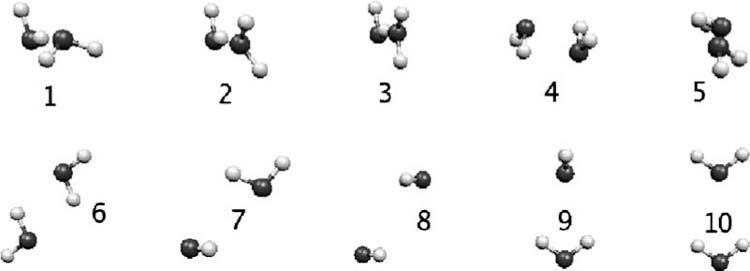
Orientation for the ten water dimers (Ref. ²⁵).

FIG. 3.

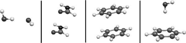
Dimers used for the 1D Coulomb and exchange-repulsion intermolecular scans.

In Sec. III A the intermolecular Coulomb interactions for all test cases are discussed. Section III B contains the results for the exchange-repulsion intermolecular interactions calculated with the overlap method, with discussion and analysis relating to the optimal fitting parameters for the frozen-core contributions. Subsequently, results for some water clusters along with timing data are presented in Sec. III C, followed by concluding remarks.

A. Intermolecular Coulomb interactions

Intermolecular Coulomb interaction results for the ten water dimers show good agreement with respect to CSOV, as can be seen in Table I (individual dimer results are reported in Supplementary Information). As can be seen, the results improve with the quality of the ABS as is to be expected. The calculated average errors for the interaction energies from Hermite coefficients are below 0.2 kcal/mol for all ABSs except for the A1 basis (see Table I), which has the smallest number of auxiliary functions per atom, in agreement with our previous results.¹⁸ Note that in the case of the ab initio densities calculated with the aug-cc-PVTZ basis, the A1, P1, and g03 basis sets do not perform as well as for densities calculated with 6−31G* basis. This is to be expected since these three ABSs are designed for double zeta basis sets. In contrast, the CFIT basis performs very well for both double zeta and triple zeta basis sets since it is designed for the latter basis sets. As can be seen from Table I the errors from the multipoles with respect to the CSOV reference values are considerably larger, around 1 kcal/mol or larger on average.

TABLE I.

Average (maximum) absolute errors in Coulomb interaction with respect to CSOV for the ten water dimers (in kcal/mol).

	6−31G*				aug-cc-pVTZ
	A1	P1	g03	CFIT	A1	P1	g03	CFIT
Hermite	0.26(0.45)	0.08(0.18)	0.02(0.09)	0.02(0.11)	0.56(1.14)	0.15(0.34)	0.12(0.28)	0.04(0.14)
Multipole	0.81(1.62)	0.79(1.73)	0.64(1.66)	1.75(3.02)	1.91(2.85)	1.65(2.29)	1.75(2.74)	1.45(2.28)

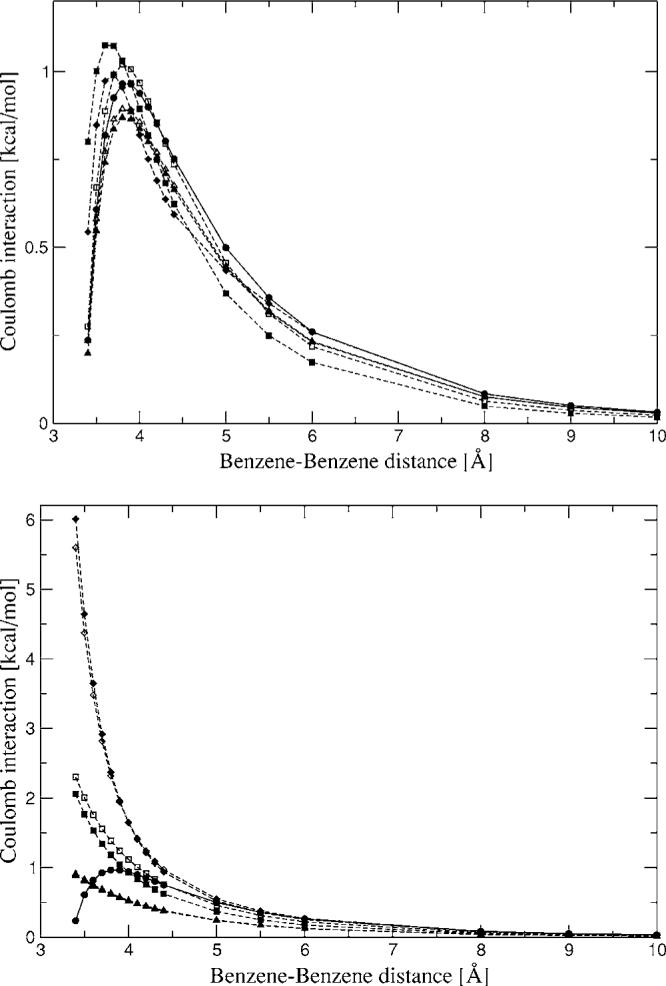
The results for the one dimensional scans for the homodimers are presented in Fig. 4–6. For the distance dependent scans (water and benzene dimers) the interactions calculated with the Hermite Gaussians show reasonable agreement with CSOV throughout the distance range. In the case of the water dimer, the short-mid- and long-range part of the curve (2.3–3.5 Å) was explored with a 0.1 Å interval; two additional points at very short range (1.5 and 1.6 Å) were also included to determine the accuracy of GEM when large penetration effects are expected. Here, as in the water dimers the accuracy at short and mid ranges goes as g03 >P1>A1 for both averaged and single fit coefficients. For example, at an O-O distance of 2.3 Å the errors are ≈1, 0.2, and 0.1 kcal/mol out of 33 kcal/mol for A1, P1, and g03, respectively. These errors shrink rapidly as the distance increases.

FIG. 4.

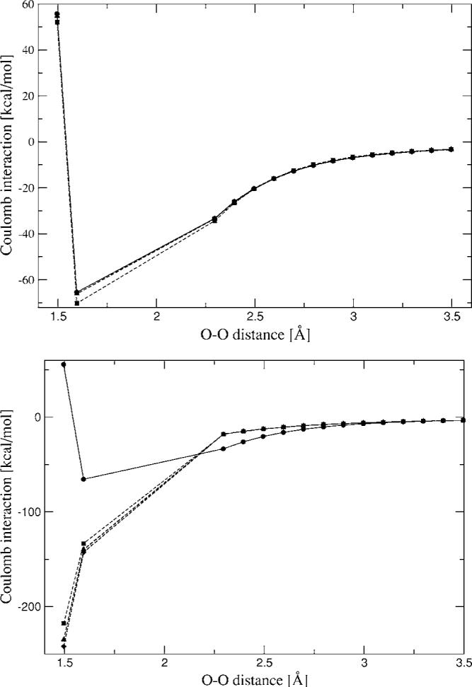
Water dimer (structure 1) Coulomb interaction energies from Hermite (top) and multipoles (bottom) for a range of distances. Closed circles—CSOV; closed squares—A1 average; open squares—A1 single; closed diamonds—P1 average; open diamonds—P1 single; closed triangles—g03 average; open triangles—g03 single.

FIG. 6.

Stacked benzene dimer Coulomb interaction energies from Hermite (top) and multipoles (bottom) for a range of distances. Closed circles—CSOV; closed squares—A1 average; open squares—A1 single; closed diamonds—P1 average; open diamonds—P1 single; closed triangles—g03 average; open triangles—g03 single.

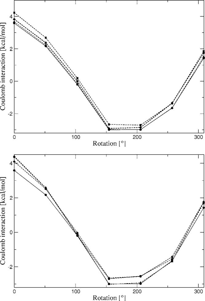
The intermolecular interactions for the rotation of the formamide dimer show reasonable agreement with the reference calculations. Hermite coefficients obtained from the fit of a single fragment as well as averaged coefficients were used for these surface scans. As can be seen, in most cases there is almost no difference between the single fit and averaged coefficients. Strangely, the only noticeable difference is for the benzene dimer at close range (Fig. 6), 3.4–3.7 Å, for the average A1 coefficients which do not reproduce the curve accurately at these distances, whereas the single fit A1 coefficients do. We currently have no explanation for this difference.

The multipolar interactions for the 1D surface scans show that these converge to the correct result at long range.

In the case of the formamide dimer rotation, we obtain good results for the Hermite interactions and relatively good results for the multipolar interactions except for the P1 derived multipoles, where the distributed multipoles for benzene show a larger deviation from the CSOV results at short and medium ranges compared with the multipoles obtained with the A1 and g03 ABSs.

The 1D surface scan for a water-benzene dimer was calculated in order to test the transferability of the Hermite coefficients (see Fig. 7). All coefficients were fitted to reproduce the intermolecular Coulomb interaction of a single homodimer, as was explained in Sec. II G. Thus, testing the Hermite coefficients on a heterodimer provides a good test for their transferability. The curve shows good agreement for the A1 and g03 ABSs along the calculated distances. In the case of the P1 Hermite coefficients a deviation of around 0.2 kcal/mol was observed at close range. This is most likely due to the fact that the carbon P1 ABS is not accurate enough for our purposes. In the case of the multipoles from P1 a large deviation is observed resulting from the poor representation of the benzene multipoles. Another interesting feature of the multipole curve for the heterodimer is that the multipoles obtained from the A1 coefficients give reasonable agreement throughout the entire distance range.

FIG. 7.

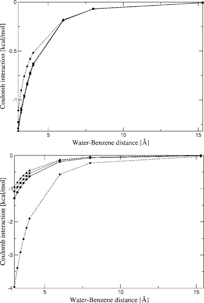
Water-benzene dimer Coulomb interaction energies from Hermite (top) and multipoles (bottom) for a range of distances. Closed circles—CSOV; closed squares—A1 average; closed diamonds—P1 average; closed triangles—g03 average.

These results show that accurate intermolecular Coulomb energies can be obtained using the DF methodology. In general the g03 ABS shows the best agreement for all test cases. The A1 ABS also shows reasonable agreement, especially for the 1D surface scans. The P1 ABS gives very accurate results for water dimer interactions but appears to break down for intermolecular Coulomb calculations with fragments containing C atoms. This could be due to the fact that we have modified the P1 ABS such that all the d orbitals in the original ABS were replaced by spd orbitals.¹⁸

B. Intermolecular exchange-repulsion interactions

As shown in Table II, good agreement is observed for the exchange-repulsion interaction calculations for the ten dimers with respect to the reference CSOV values in general (see Supplementary Information for individual dimers). However, note that better results are obtained if the Hermite coefficients are fitted to reproduce the exchange-repulsion interaction for the A1 basis, which is the smallest ABS. The reason is that even though the fitted density calculated with the parameters for the Coulomb fit is good, the errors (see Supplementary Materials for color scales) extend further from the molecule than for the exchange-repulsion parameters, as can be seen in Fig. 8. This is in agreement with the fact that only the valence density is needed for the determination of the exchange repulsion using the overlap model, as explained by Wheatley and Price.²⁵ The exact and fitted density cubes for the comparison in Fig. 8 were obtained with density matrices from GAUSSIAN 98 at the B3LYP/6−31G* level.⁷⁰ Better results were also observed in the case of the P1 ABS with aug-cc-PVTZ by optimizing the Hermite coefficients for exchange repulsion. However, in this case the difference is much less: 0.14 kcal/mol average error with Hermite coefficients optimized for exchange repulsion (see Table II) compared with 0.19 kcal/mol average error for Hermite coefficients optimized for Coulomb. On the other hand, for the rest of the cases, the same Hermite coefficients give the best Coulomb and exchange-repulsion interaction results.

TABLE II.

Average (maximum) absolute errors in exchange-repulsion interaction with respect to CSOV for the ten water dimers (in kcal/mol).

6−31G*			aug-cc-PVTZ
A1	P1	g03	A1	P1	g03
0.15(0.24)	0.18(0.55)	0.14(0.43)	0.41(0.72)	0.14(0.22)	0.21(0.79)

FIG. 8.

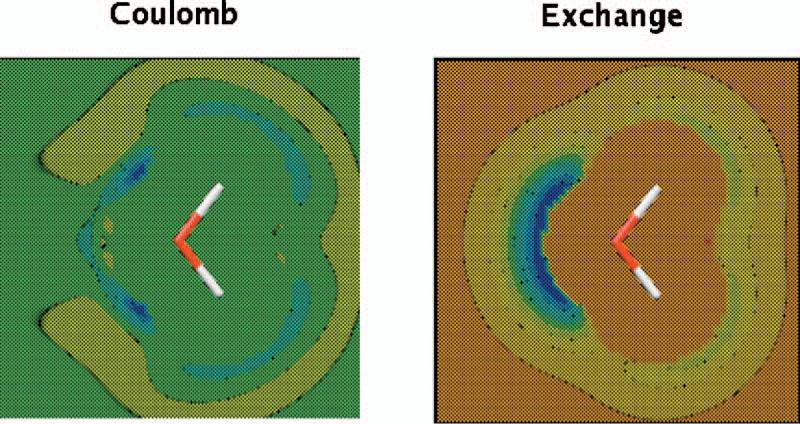
(Color) Water molecule density difference maps for density fitting using A1 ABS with respect to ab initio. All calculations and fittings were done at the B3LYP/6−31G* level with a fine grid (120×120×120 points). All density fitting results were obtained using midpoints with O ABS.

The errors for the exchange-repulsion interactions presented in Table II are not as good as the ones obtained for GEM-0.²² This is probably due to the fact that the training set for the linear regression in the calculation of the K parameter was significantly smaller in the present study than for the GEM-0 parametrization, only ten dimers in the present study compared to 190 random orientations. Nevertheless, note that the errors for the results obtained with the λ optimized for exchange repulsion are around 0.2–0.3 kcal/mol for the three ABSs when fitting 6−31G* density. The errors for the fit of the aug-cc-pVTZ are bigger; this is most likely due to the fact that the three ABSs used for this interaction are designed to work with double zeta basis sets as noted in Sec. III A.

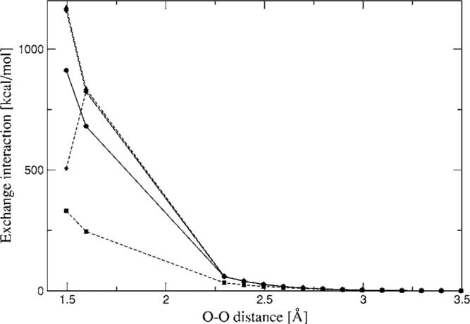
The 1D homodimer surface scans are presented in Figs. 9–11. Both distance dependent scans (water and benzene dimers) show reasonable agreement with CSOV along a wide range of distances, especially for benzene. In the case of water dimer 1 (Fig. 9), the simple overlap model with fitted densities begins to break down at short to very short range. However it is important to note that there is strong dependence on the ABS quality, for example, the errors at 2.5 Å are around 30% for A1, 4% for P1, and 2% for g03. At 2.7 Å (hydrogen bonding distance) these errors are reduced to 10% for A1 and remain around 2%–3% for P1 and g03. For longer distances the errors are reduced to less than 2% (0.2 kcal/mol and below) for all auxiliary basis sets. The 1D homodimer scan for rotation (Fig. 10) shows that all three ABSs follow the shape of the reference curve. In all cases the largest errors of the intermolecular exchange interactions with respect to CSOV are around 0.2 kcal/mol.

FIG. 9.

Water dimer (structure 1) exchange-repulsion interaction energies for a range of distances. Closed circles—CSOV; stars—ab initio density; closed squares—A1 single; closed diamonds—P1 single; closed triangles— g03 single.

FIG. 11.

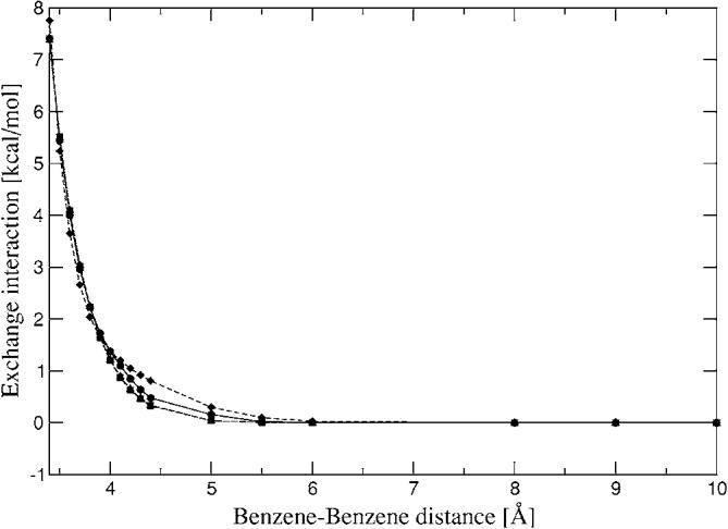
Stacked benzene dimer exchange-repulsion interaction energies for a range of distances. Closed circles—CSOV; closed squares—A1 single; closed diamonds—P1 single; closed triangles—g03 single.

FIG. 10.

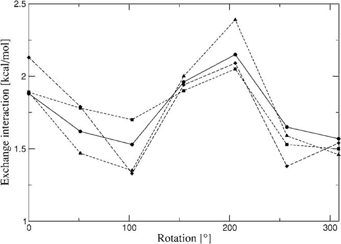
Formamide exchange-repulsion interaction energies rotating about one of the fragments. Closed circles—CSOV; closed squares—A1 single; closed diamonds—P1 single; closed triangles—g03 single.

Additionally, the intermolecular exchange repulsion for water dimer 1 has been calculated with the overlap model using the full ab initio density, as shown in Fig. 9. In this case the overlap model agrees very well with CSOV results in the range of 2.3–3.5 Å, with errors below 1%. At very short distances (1.6 Å and below) the errors increase substantially. Based on these results it can be seen that this simple model is very robust even at smaller intermolecular distances than those encountered in regular hydrogen bonding situations and the intermolecular exchange-repulsion interactions calculated with fitted densities will depend on the quality of the fitted densities and not on the accuracy of the overlap model.

As can be seen from Fig. 12, the exchange-repulsion interaction for the water-benzene heterodimer surface agrees with the reference curve. In all cases the average errors are below 0.15 kcal/mol. Note that in the case of the P1 ABS, very small negative values (>0.02 kcal/mol) are observed at 3.6 and 4.0 Å; this is due to the error on the benzene coefficients for this ABS. Also, in this case a small kink is observed in the CSOV curve, this is most likely due to the fact that the integration grid for the B3LYP calculation was not fine enough. This kink is also the reason why the R² obtained for the linear regressions to determine the K parameters are in the order of 0.95 instead of 0.99 as obtained for all the homodimer linear regressions (see Supplementary Materials). In spite of this we observe reasonable agreement with respect to the reference calculation.

FIG. 12.

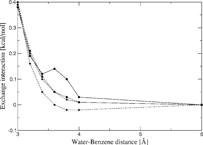
Water-benzene dimer exchange-repulsion interaction energies for a range of distances. Closed circles—CSOV; closed squares—A1 average; closed diamonds—P1 average; closed triangles—g03 average.

C. Reciprocal space calculations

The implementation of GEM with the reciprocal space methods has been tested by calculating the intermolecular Coulomb energy and force for a series of water boxes, (H₂O)_n, n=64, 128, 256, 512, and 1024, in PBC. In practice in the molecular dynamics (md) community, the measure of the accuracy for a force field has been the force since this is the quantity that will determine the md trajectories. Additionally, there have been recent proposals for force field parametrization using force matching.^71,72

Initially the accuracy of the forces calculated with GEM with three ABSs has been determined by comparing the calculated GEM forces with forces obtained with CSOV using the finite difference method. Table III shows the rms deviation for the ten water dimers between forces calculated with A1, P1, and g03 ABSs versus the CSOV forces from molecular density calculated with 6−31G* and aug-cc-pVTZ basis sets for both Coulomb and overlap interactions (see Supplementary Information for complete tables). In the case of the Coulomb interaction, as observed previously, the accuracy increases when better ABSs are employed for both basis sets. Furthermore, the rms between the CSOV forces obtained with the two different basis sets is 0.14, compared with the largest rms at the 6−31G* level obtained with A1 of 0.06 (see Table III). In the case of the aug-cc-pVTZ densities, A1 shows a slightly larger rms (0.15); however, as explained previously, all three ABSs are designed to work with double zeta basis. Both P1 and g03 show slightly larger rms with respect to CSOV with the larger basis set although it is still well below the CSOV one.

TABLE III.

Relative rms force deviation with respect to CSOV for the ten water dimers.

	6−31G*			aug-cc-pVTZ
	A1	P1	g03	A1	P1	g03
Coulomb	0.06	0.03	0.01	0.15	0.04	0.05
Exchange	0.22	0.08	0.07	0.12	0.04	0.07

For the overlap forces the CSOV rms deviation obtained between 6−31G* and aug-cc-pVTZ is considerably larger, 0.26. In this case the rms for all ABSs using both basis sets is below the CSOV rms. Note that, as was the case above, the results for overlap are not as good as for Coulomb interactions. Also note that in this case the use of reciprocal space methods for the overlap determination results only in a modest improvement in computational efficiency. For example, the overlap energy force for the 256 water box to 10⁻⁴ rms force tolerance with the P1 ABS calculating all integrals in direct space takes 1.88 s; on the other hand, when using reciprocal space methods the time is reduced to 1.31 s.

Figures 13 and 14 show the CPU time for a single energy-force Coulomb calculation for the water boxes in PBC using relative rms force tolerances of 10⁻³ and 10⁻⁴ respectively. These tolerances were chosen to be well below the intrinsic accuracy of the ABS fits of 1%–10%. All calculations were performed on a single CPU of a dual Xeon 3.3 GHz computer with 3 Gbytes of memory. In both cases the A1 and P1 ABSs show a quasilinear behavior for both the PME and FFP methods for all boxes, while g03 gives a quasilinear behavior for FFP and linear behavior for PME up to 512 waters and quadratic afterward. Note first that unlike previous PME implementations, in the present case the reciprocal space calculations dominate the compute time. Thus the irregularities in feasible FFT grid dimensions (restricted to products of powers of 2, 3, and 5) result in nonsmooth timings as a function of system size. Furthermore, currently the code does not allow for cutoffs bigger than 1/2 the box size which limits timing optimization in the 64 and 128 water boxes. The quadratic behavior is most probably due to an inefficient use of memory in our code due to the large Hermite-Hermite interaction list which is kept in memory, as well as the large number of FFTs required. We have decided not to report results obtained with the Ewald method since it is too slow [O(N²) scaling] compared to FFT and PME. Interestingly, from the results it is observed that the advantage of PME widens for more accurate results (10⁻⁴ rms) compared to FFP because in this case it is difficult to increase accuracy with the Gaussian splitting method and the increase of accuracy in FFP requires a better sampling of the tails of the Gaussians. Also, note that in the case of the Coulomb calculation, in order to achieve a relative rms of 10⁻⁴ the rms accuracy of the individual components (e-e and N-e) needs to be equivalent to 5×10⁻⁸ due to the fact that a subtraction between very large numbers has to be performed. For example, for dimer 1 the e-e, N-N, and N-e energies are approximately 18.285, 18.325, and −36.624 hartree compared with −8.32 kcal/mol for the total Coulomb interaction.

FIG. 13.

Timings for water boxes with rms force tolerance of 10⁻³. Closed circles—A1 PME; closed squares—P1 PME; closed diamonds—g03 PME; open circles—A1 FFP; open squares—P1 FFP; open diamonds—g03 FFP.

FIG. 14.

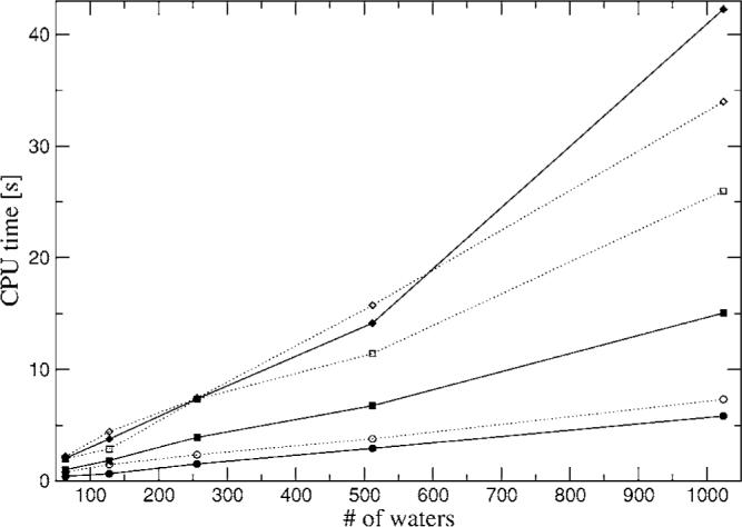
Timings for water boxes with rms force tolerance of 10⁻⁴. Closed circles—A1 PME; closed squares—P1 PME; closed diamonds—g03 PME; open circles—A1 FFP; open squares—P1 FFP; open diamonds—g03 FFP.

The reciprocal space methods are quite efficient. The calculation of the energy and force for the largest system tested at the highest accuracy, i.e., the 1024 water box with g03 ABS, which corresponds to 654 336 Hermite coefficients, takes only 34 s with FFP and 42 s with PME (see Fig. 14). Moreover, note that both reciprocal space methods are highly parallelizable, which would increase the computational efficiency. Additionally, we have not explored the possibility of using FFTW for PME which would allow the calculation of multiple FFTs at once, as well as a thorough optimization of all the possible parameters involved in the FFP implementation with Gaussian splitting. Another factor that could be used to decrease the FFP computing time is the addition of a third level coarse grid when the ABSs have very diffuse auxiliary basis. Finally, it is important to mention that results obtained with both PME and FFP can be mixed (data not shown); therefore this opens up interesting possibilities such as a QM/MM implementation using GEM,⁴⁵ where the GEM section proximal to the QM can be calculated with PME or FFP, while the rest of the MM subsystem can be represented via GEM multipoles and calculated in reciprocal space with PME (work in progress).

IV. CONCLUSIONS

The Gaussian electrostatic model has been extended for use of Hermite Gaussian fitting functions of arbitrary angular momentum. In addition to increased computational speed by the use of the generalized MD recursion, the use of Hermite Gaussians also gives rise to the determination of site multipoles obtained directly from the fitting procedure. Noise problems for the fit of the expansion coefficients have been addressed by using the Tikhonov regularization method as well as by means of the damped Coulomb kernel. The use of a local reference frame for each fitting site allows the rotation of the fitting coefficients in order to perform intermolecular interaction calculations. Frozen-core intermolecular contributions (Coulomb and exchange repulsion) have been calculated for a series of systems including both homo- and heterodimers. Three different fitting basis sets were tested for accuracy. Reasonable agreement is obtained in all cases for the intermolecular interactions with errors below 0.1 kcal/mol for electrostatic and around 0.15–0.2 kcal/mol for exchange repulsion. Additionally, a significant computational speedup is achieved by using reciprocal space methods. Three such methods were implemented, FFP, PME, and regular Ewald. Results for a series of water boxes in PBC using rms accuracies of 10⁻³ and 10⁻⁴ have been obtained and the CPU timings have been reported. For example, a 1024 water box using the g03 ABS (the largest system and ABS studied) takes 42 s for an energy-force calculation with PME and 34 s with FFP.

FIG. 5.

Formamide dimer Coulomb interaction energies from Hermite (top) and multipoles (bottom) rotating about one of the fragments. Closed circles—CSOV; closed squares—A1 average; open squares—A1 single; closed diamonds—P1 average; open diamonds—P1 single; closed triangles—g03 average; open triangles—g03 single.

References

- 1.Case DA, Cheatham TE, III, Darden TA, Gohlke H, Luo R, Merz KM, Jr., Onufirev A, Simmerling C, Wang B, Woods RJ. J. Comput. Chem. 2005;26:1668. doi: 10.1002/jcc.20290. [DOI] [PMC free article] [PubMed] [Google Scholar]
- 2.Jorgensen WL, Tirado-Rives J. J. Comput. Chem. 2005;26:1669. doi: 10.1002/jcc.20297. [DOI] [PubMed] [Google Scholar]
- 3.van der Spoel D, Lindahl E, Hess B, Groenhoff G, Mark AE, Berensen HJC. J. Comput. Chem. 2005;26:1701. doi: 10.1002/jcc.20291. [DOI] [PubMed] [Google Scholar]
- 4.Christen M, Hünenberger PH, Bakowies D, et al. J. Comput. Chem. 2005;26:1719. doi: 10.1002/jcc.20303. [DOI] [PubMed] [Google Scholar]
- 5.MacKerrell AD, Jr., Brooks B, Brooks CL, III, Roux NB, Won Y, Karplus M. Encyclopedia of Computational Chemistry. Wiley; NewYork, NY: 1998. [Google Scholar]
- 6.Leach AR. Molecular Modelling: Principles and Applications. 2nd ed. Prentice-Hall; Harlow, UK: 2001. [Google Scholar]
- 7.Stone AJ. The Theory of Intermolecular Forces. Oxford University Press; Oxford, UK: 2000. [Google Scholar]
- 8.Stone AJ. Chem. Phys. Lett. 1981;83:233. [Google Scholar]
- 9.Vigné-Maeder F, Claverie P. J. Chem. Phys. 1988;88:4934. [Google Scholar]
- 10.Náray-Szabó G, Ferenczy GG. Chem. Rev. Vol. 95. Washington, D.C.: 1995. p. 829. [Google Scholar]
- 11.Gresh N, Claverie P, Pullman A. Int. J. Quantum Chem. 1979;22:253. [Google Scholar]
- 12.Gresh N. J. Comput. Chem. 1995;16:856. [Google Scholar]
- 13.Ren P, Ponder JW. J. Phys. Chem. B. 2003;107:5933. [Google Scholar]
- 14.Freitag MA, Gordon MS, Jensen JH, Stevens WJ. J. Chem. Phys. 2000;112:7300. [Google Scholar]
- 15.Piquemal J-P, Gresh N, Giessner-Prettre C. J. Phys. Chem. A. 2003;107:10353. doi: 10.1021/jp035748t. [DOI] [PubMed] [Google Scholar]
- 16.Gresh N, Piquemal J-P, Krauss M. J. Comput. Chem. 2005;26:1113. doi: 10.1002/jcc.20244. [DOI] [PubMed] [Google Scholar]
- 17.Gavezzotti A. J. Phys. Chem. B. 2002;106:4145. [Google Scholar]
- 18.Cisneros GA, Piquemal J-P, Darden TA. J. Chem. Phys. 2005;123:044109. doi: 10.1063/1.1947192. [DOI] [PMC free article] [PubMed] [Google Scholar]
- 19.Boys SF, Shavit I. A Fundamental Calculation of the Energy Surface for the System of Three Hydrogens Atoms. NTIS; Springfield, VA: 1959. p. AD212985. [Google Scholar]
- 20.Dunlap BI, Connolly JWD, Sabin JR. J. Chem. Phys. 1979;71:4993. [Google Scholar]
- 21.Köster AM, Calaminici P, Gómez Z, Reveles U. Reviews of Modern Quantum Chemistry: A Celebration of the Contribution of Robert G. Parr. World Scientific; Singapore: 2002. [Google Scholar]
- 22.Piquemal J-P, Cisneros GA, Reinhardt P, Gresh N, Darden TA. J. Chem. Phys. 2006;124:104101. doi: 10.1063/1.2173256. [DOI] [PMC free article] [PubMed] [Google Scholar]
- 23.Bagus PS, Hermann K, Bauschlicher CW., Jr. J. Chem. Phys. 1984;80:4378. [Google Scholar]
- 24.Piquemal J-P, Marquez A, Parisel O, Giessner-Prettre C. J. Comput. Chem. 2005;26:1052. doi: 10.1002/jcc.20242. [DOI] [PubMed] [Google Scholar]
- 25.Wheatley RJ, Price SL. Mol. Phys. 1990;69:507. [Google Scholar]
- 26.Domene C, Fowler PW, Wilson M, Madden P, Wheatley RJ. Chem. Phys. Lett. 2001;333:403. [Google Scholar]
- 27.Tschumper GS, Leininger ML, Hoffman BC, Valeev EF, Schaffer HF, III, Quack M. J. Chem. Phys. 2002;116:690. [Google Scholar]
- 28.van Duijneveldt–van de Rijdt JGCM, Mooij WTM, Duijneveldt FB. Phys. Chem. Chem. Phys. 2003;5:1169. [Google Scholar]
- 29.Press WH, Teukolsky SA, Vetterling WT, Flannery BP. Numerical Recipes in Fortran77: The Art of Scientific Computing. 2nd ed. Cambridge University Press; New York, NY: 1992. [Google Scholar]
- 30.Jung Y, Sodt A, Gill PMW, Head-Gordon M. Proc. Natl. Acad. Sci. U.S.A. 2005;102:6692. doi: 10.1073/pnas.0408475102. [DOI] [PMC free article] [PubMed] [Google Scholar]
- 31.Helgaker T, Jørgensen PJ, Olsen J. Molecular Electronic-Structure Theory. Wiley; Chichester, England: 2000. [Google Scholar]
- 32.Köster AM. J. Chem. Phys. 2003;118:9943. [Google Scholar]
- 33.McMurchie LE, Davidson ER. J. Comput. Phys. 1978;26:218. [Google Scholar]
- 34.Tachikawa M, Shiga M. Phys. Rev. E. 2001;64:056707. doi: 10.1103/PhysRevE.64.056706. [DOI] [PubMed] [Google Scholar]
- 35.Trickey SB, Alfort JA, Boettger JC. Computational Materials Science. Elsevier B. V.; Amsterdam: 2004. [Google Scholar]
- 36.Sagui C, Pedersen LG, Darden TA. J. Chem. Phys. 2004;120:73. doi: 10.1063/1.1630791. [DOI] [PubMed] [Google Scholar]
- 37.Eichkorn K, Treutler O, Öhm H, Häser M, Ahlrichs R. Chem. Phys. Lett. 1995;240:283. [Google Scholar]
- 38.Köster AM. J. Chem. Phys. 1996;104:4114. [Google Scholar]
- 39.Podeszwa R, Bukowski R, Szalewicz K. J. Chem. Theory Comput. 2006;2:400. doi: 10.1021/ct050304h. [DOI] [PubMed] [Google Scholar]
- 40.Misquitta AJ, Stone AJ. J. Chem. Phys. 2006;124:024111. doi: 10.1063/1.2150828. [DOI] [PubMed] [Google Scholar]
- 41.Arfken G, Weber H. Mathematical Methods for Physicists. Academic; San Diego, CA: 1996. [Google Scholar]
- 42.Toukmaji A, Sagui C, Board J, Darden TA. J. Chem. Phys. 2000;113:10913. [Google Scholar]
- 43.Ángyán JG, Chipot C, Dehez F, Hätig C, Jansen G, Millot C. OPEP, a tool for the optimal partitioning of electric properties, Version 1.0-β, Equipe de Chimie and Biochimie Théoretiques, Unité Mixte de Recherche CNRS/UHP No. 7565. Université Henri Poincaré; France: 2005. [Google Scholar]
- 44.Challacombe M, Schwgler E, Almlöf J. Computational Chemistry: Review of Current Trends. World Scientific; Singapore: 1996. [Google Scholar]
- 45.Cisneros GA, Piquemal J-P, Darden TA. J. Phys. Chem. B. 2006;110:13682. doi: 10.1021/jp062768x. [DOI] [PMC free article] [PubMed] [Google Scholar]
- 46.Stone AJ. J. Chem. Theory Comput. 2005;1:1128. doi: 10.1021/ct050190+. [DOI] [PubMed] [Google Scholar]
- 47.Popelier PLA, Joubert L, Kosov DS. J. Phys. Chem. A. 2001;105:8524. [Google Scholar]
- 48.Volkov A, Coppens P. J. Comput. Chem. 2004;25:921. doi: 10.1002/jcc.20023. [DOI] [PubMed] [Google Scholar]
- 49.Clementi E. Computational Aspects of Large Chemical Systems. Springer; New York, NY: 1980. [Google Scholar]
- 50.Dupuis M, Marquez A, Davidson ER. HONDO95.3, quantum chemistry program exchange (QCPE) Indiana University; Bloomington, IN: 1995. [Google Scholar]
- 51.Fusti-Molnar L, Pulay P. J. Chem. Phys. 2002;117:7827. [Google Scholar]
- 52.Lippert D, Hutter J, Parrinello M. Theor. Chem. Acc. 1999;103:124. [Google Scholar]
- 53.Krack M, Parrinello M. Phys. Chem. Chem. Phys. 2000;2:2105. [Google Scholar]
- 54.Cohen-Tannoudji C, Diu B, Laloe F. Quantum Mechanics. Wiley Interscience; New York, NY: 1977. [Google Scholar]
- 55.Ahlrichs R. Phys. Chem. Chem. Phys. 2006;8:3072. doi: 10.1039/b605188j. [DOI] [PubMed] [Google Scholar]
- 56.Essmann U, Perera L, Berkowitz M, Darden TA, Lee H, Pedersen LG. J. Chem. Phys. 1995;103:8577. [Google Scholar]
- 57.York D, Yang W. J. Chem. Phys. 1994;101:3298. [Google Scholar]
- 58.Shan YB, Klepis JL, Eastwood MP, Dror RO, Shaw DE. J. Chem. Phys. 2005;122:054101. doi: 10.1063/1.1839571. [DOI] [PubMed] [Google Scholar]
- 59.Smith ER. J. Stat. Phys. 1994;77:449. [Google Scholar]
- 60.Sagui C, Darden TA. J. Chem. Phys. 2001;114:6578. [Google Scholar]
- 61.Amos RD, Alberts IL, Andrews JS, et al. CADPAC, the Cambridge analytic derivatives package, Issue 6. Cambridge University; Cambridge, UK: 1995. [Google Scholar]
- 62.Becke AD. J. Chem. Phys. 1993;98:5648. [Google Scholar]
- 63.Lee C, Yang W, Parr RG. Phys. Rev. B. 1988;37:785. doi: 10.1103/physrevb.37.785. [DOI] [PubMed] [Google Scholar]
- 64.Andzelm J, Wimmer E. J. Chem. Phys. 1992;96:1280. [Google Scholar]
- 65.Godbout N, Andzelm J. DGAUSS, Versions 2.0, 2.1, 2.3, and 4.0. Computational Chemistry List, Ltd.; Columbus, OH: 1998. http://www.ccl.net/cca/data/basis-sets/DGauss/index.shtml the file that contains the A1 and P1 auxiliary basis sets can be obtained from the CCL WWW site at. [Google Scholar]
- 66.Frisch MJ, Trucks GW, Schlegel HB, et al. GAUSSIAN 03. Gaussian, Inc.; Pittsburgh, PA: 2003. [Google Scholar]
- 67.Berholdt DE, Harrison RJ. J. Chem. Phys. 1998;109:1593. [Google Scholar]
- 68.Jorgensen W, Chandrasekhar J, Madura J, Impey R, Klein M. J. Chem. Phys. 1983;79:926. [Google Scholar]
- 69.Ponder J. TINKER, software tools for molecular design, Version 3.6. Washington University; St. Louis, MO: 1998. http://dasher.wustl.edu/tinker the most updated version for the TINKER program can be obtained from J. Ponder's WWW site at. [Google Scholar]
- 70.Frisch MJ, Trucks GW, Schlegel HB, et al. GAUSSIAN 98, Revision A.8. Gaussian, Inc.; Pittsburgh, PA: 1998. [Google Scholar]
- 71.Ercolessi R, Adams JB. Europhys. Lett. 1994;26:583. [Google Scholar]
- 72.Laio A, Bernard S, Chiarotti CL, Scandolo S, Tosatti E. Science. 2000;287:1027. doi: 10.1126/science.287.5455.1027. [DOI] [PubMed] [Google Scholar]
- 73.Also, it is important to note that we rely on the exponents of the diffuse functions to be smaller than α0 to ensure uniform convergence in the sums of Eq. (29). That is, if 1/αd>1/α0 these sums converge uniformly.
- 74.See EPAPS Document No. E-JCPSA6−125−309641 for the optimal fitting parameters for all molecules tested in this study; intermolecular Coulomb and exchange-repulsion results for individual water dimers; K parameters for exchange repulsion for all fragments; scales for density comparison cubes; Coulomb and overlap forces for CSOV and the three ABSs. This document can be reached via a direct link in the online article's HTML reference section or via the EPAPS homepage (http://www.aip.org/pubservs/epaps.html).