“New-version-fast-multipole-method” accelerated electrostatic interactions in biomolecular systems

Abstract

In this paper, we present an efficient and accurate numerical algorithm for calculating the electrostatic interactions in biomolecular systems. In our scheme, a boundary integral equation (BIE) approach is applied to discretize the linearized Poisson-Boltzmann (PB) equation. The resulting integral formulas are well conditioned for single molecule cases as well as for systems with more than one macromolecule, and are solved efficiently using Krylov subspace based iterative methods such as generalized minimal residual (GMRES) or bi-conjugate gradients stabilized (BiCGStab) methods. In each iteration, the convolution type matrix-vector multiplications are accelerated by a new version of the fast multipole method (FMM). The implemented algorithm is asymptotically optimal O(N) both in CPU time and memory usage with optimized prefactors. Our approach enhances the present computational ability to treat electrostatics of large scale systems in protein-protein interactions and nano particle assembly processes. Applications including calculating the electrostatics of the nicotinic acetylcholine receptor (nAChR) and interactions between protein Sso7d and DNA are presented.

1 Introduction

In this paper, we discuss a numerical algorithm for the calculation of electrostatic interactions in biomolecular systems in solution, in which the solvent has a substantial volume with numerous mobile ions making significant contributions. Such systems are commonly encountered in biophysics, electrochemistry, and electrophoresis, such as in the study of protein-protein interactions and nano particle assembly processes in drug design and structural biology.

Although the continuum Poisson-Boltzmann (PB) equation model for these systems was introduced almost a century ago by Debye and Hückel¹⁷ and later developed by Kirkwood,²⁶ its numerical solutions have only been extensively explored in the last two decades.^{13, 16, 19, 23, 24, 27, 40, 46, 48} Traditional schemes include the finite difference methods where difference approximations are used on structured grids describing the computational domain, and finite element methods in which arbitrarily shaped biomolecules are discretized using elements and associated basis functions. The resulting algebraic systems for both are commonly solved using multigrid or domain decomposition accelerations for optimal efficiency. However, as the grid number (and thus the storage, number of operations, and condition number of the system) increases proportionally to the volume size, finite difference and finite element methods become less efficient and accurate for systems of large spatial sizes commonly encountered in studying either macromolecules or interacting systems in the association and dissociation processes. Alternative methods include the boundary element (BEM) and boundary integral equation (BIE) methods. In these methods, only the surfaces (compared to the 3D volume) of the molecules are discretized and hence the number of unknowns is greatly reduced. In addition, the boundary elements (BEs) form a kind of surface “conforming” mesh (because they align with the surface), which therefore allows the application of the BEM to biomolecules characterized by irregular geometries, while maintaining a high level of calculation accuracy.

However, in practical biomodeling, the BEM is the least used relative to the other methods. In earlier versions of BEM, the integral equation formulations may not have been well-conditioned and the matrix was typically stored explicitly. The resulting dense linear system was often solved using direct matrix inversion such as Gauss elimination or LU decompsition, so that O(N²) storage and O(N³) operations were required, where N is the number of unknowns defined on the surface. This is extremely inefficient for any typical size system of interest. To improve the BEM efficiency, some later studies improved the condition of the integral formulation,^{2, 24, 29, 30} reduced the number of the boundary elements⁴⁴ or introduced novel BEM.³¹ It has been dmonstrated that when the system is well-conditioned or can be effectively preconditioned, the matrix equations can be solved efficiently using iterative Krylov subspace methods which are matrix-implicit, thus eliminating the bottleneck of storage. As the number of iterations in these methods is independent of the system size for well conditioned systems, the computational cost is then dominated by the matrix-vector multiplication calculations corresponding to the N-body electrostatic particle interactions of both the Coulombic (κ = 0) and screened Coulombic (κ ≠ 0) types, which require O(N²) operations using direct methods for each iteration. By introducing novel fast summation algorithms developed in the last twenty years, this cost has been reduced to O(N log N). These algorithms incude the hierarchical “tree code”,^{4, 6} fast Fourier transform (FFT) based algorithms such as the precorrected FFT (pFFT)^{3, 28, 35} and the particle-mesh Ewald (PME) methods,¹⁵ the hierarchical SVD method,²⁵ and FFT on multipoles.^{33, 34} Further improvements show that asymptotically optimal O(N) complexity can be achieved by using the wavelet techniques^{41, 43} or the fast multipole method (FMM).²⁰ FMM algorithms for the screened Coulombic interaction (Yukawa potential) have also been recently developed,^{9, 22} which allows their direct application to the solution of the PB equation. The tree code algorithm and the FMMs based on the old scheme²⁰ have been implemented in former BEM PB work.^{7, 8, 10, 18, 34, 49} However, as revealed by previous numerical experiments, although asymptotically optimal, the original FMM²⁰ turns out to be less efficient for problem sizes of current interest when compared with the tree code and FFT based O(N log N) techniques, due to the huge prefactor in O(N).¹⁸

To further accelerate the numerical solution of the PB equation, in this paper, we present an efficient algorithm using a well conditioned BIE formulation, for which the solution is accelerated by a new version of FMM first introduced by Greengard and Rokhlin²¹ for the Laplace equation. By proper coupling of single and double layer potentials as in ref. 38, a Fredholm second kind integral equation formulation for the PB equation can be derived. Similar formulations were first introduced by Juffer et al.²⁴ who aimed to avoid the singularity problem in deriving the complete BIE forms for the linearized PB equation. The well-conditioned property has been discussed by Liang et al.,²⁹ and also demonstrated in the work of Boschitsch et al.¹⁰ We extend the formulation for systems with an arbitrary number of domains. Compared with traditional BEM formulations, the condition number of our BIE system does not increase with the number of unknowns, hence the number of iterations in the Krylov subspace based methods is bounded. For the matrix vector multiplication in each iteration, we use the new version FMM developed for the screened Coulombic interaction (Yukawa potential).²² Compared with the original FMM, the plane wave expansion based diagonal translation operators dramatically reduce the prefactor in the O(N) new version FMM, especially in three dimensions where a break-even point of approximately 600 for 6 digits precision is numerically observed. Perhaps due to its complexity in theory and programming, we are unaware of any previous implementations of the new version FMM for the PB equation.

This paper is organized as follows. In Sec. 2, we discuss the methodological details of our algorithm, including the well-conditioned integral equation formulation and the new version of FMM. In Sec. 3, the resulting algorithm is applied to both a single protein and a two-molecule (protein-DNA) interaction cases to illustrate the performance of the algorithm. Finally in Sec. 4, conclusions and discussion are presented. We want to mention that some of the analyses were briefly reported previously in ref. 30. The purpose of this paper is to present more technical details along with two new applications.

2 Methods

In this section, we discuss the technical details of the algorithm. In particular, the boundary integral equation formulation and its discretization, the new version of FMM and how it is applied to the BEM, the Krylov subspace method, the mesh generation, and the system set up are discussed in order.

2.1 Boundary integral equation formulations

When Green’s second identity is applied, traditional boundary integral equations for the linearized PB equation for a single domain (molecule) take the form

$$\frac{1}{2}{\phi }_p^{int}={\oint }_S^{PV}[G_{pt}\frac{\partial {\phi }_i^{int}}{\partial n}-\frac{\partial G_{pt}}{\partial n}{\phi }_t^{int}]d{S}_t+\frac{1}{D_{int}}\sum _k{q}_k{G}_{pk},\hspace{0.17em}\hspace{0.17em}\hspace{0.17em}p\in S,$$ (1)

$$\frac{1}{2}{\phi }_p^{\text{ext}}={\oint }_S^{PV}[-u_{pt}\frac{\partial {\phi }_t^{\text{ext}}}{\partial n}-\frac{\partial u_{pt}}{\partial n}{\phi }_t^{\text{ext}}]d{S}_t,\hspace{0.17em}\hspace{0.17em}\hspace{0.17em}p\in S,$$ (2)

where ${\phi }_p^{int}$ is the interior potential at surface position p of the molecular domain Ω, S = ∂Ω is its boundary, i.e., solvent-accessible surface, ${\phi }_p^{\text{ext}}$ is the exterior potential at position p, D_int is the interior dielectric constant, t is an arbitrary point on the boundary, n is the outward normal vector at t, and PV represents the principal value integral to avoid the singular point when t → p in the integral equations. In the formulae, $G_{pt}=\frac{1}{4\pi \mid r_t-r_p\mid }$ and $u_{pt}=\frac{exp(-\kappa \mid r_t-r_p)}{4\pi \mid r_t-r_p\mid }$ are the fundamental solutions of the corresponding Poisson and Poisson-Boltzmann equations, respectively, r_k is the position of the kth source point charge q_k of the molecule, κ is the reciprocal of the Debye-Hückel screening length determined by the ionic strength of the solution. These equations can be easily extended to multi-domain systems in which Eq. (1) is enforced for each individual domain and the integration domain in Eq. (2) includes the collection of all boundaries.³²

To complete the system, the solutions in the interior (Eq. (1)) and exterior (Eq. (2)) are matched by the boundary conditions φ^int = φ^ext and $D_{int}\frac{\partial {\phi }^{int}}{\partial n}=D_{\text{ext}}\frac{\partial {\phi }^{\text{ext}}}{\partial n}$, where D_ext is the exterior (solvent) dielectric constant. Using these conditions, we can define f = φ^ext and $h=\frac{\partial {\phi }^{\text{ext}}}{\partial n}$ as the new unknowns and recover other quantities using boundary integrals of f and h. Unfortunately, theoretical analysis shows that the corresponding equation system for f and h is in general a Fredholm integral equation of first kind and hence ill-conditioned. i.e., when solved iteratively using Krylov subspace methods, the number of iterations increases with the number of unknowns, and the resulting algorithm becomes inefficient for large systems. Instead of this “direct formulation”, Rokhlin³⁸ introduced a technique where the single and double layer potentials are combined in order to derive an optimized second kind Fredholm integral equation. We want to mention that a well-conditioned form actually appeared in Juffer et al.’s work²⁴ when they tried to derive the complete BI form for linearized PBE using a limiting process to avoid the singularity problem. The same form has been used and discussed in later BEM PB work,^{10, 29} and similar techniques have also been applied and discussed in engineering computations.⁴²

The derivative BEM (dBEM) can be obtained by linearly combining the derivative forms of Eqs. (1)–(2):

$$(\frac{1}{2\epsilon }+\frac{1}{2})f_p={\oint }_S^{PV}[(G_{pt}-u_{pt})h_t-(\frac{1}{\epsilon }\frac{\partial G_{pt}}{\partial n}-\frac{\partial u_{pt}}{\partial n})f_t]d{S}_t+\frac{1}{D_{\text{ext}}}\sum _k{q}_k{G}_{pk},\hspace{0.17em}\hspace{0.17em}\hspace{0.17em}p\in S,$$ (3)

$$(\frac{1}{2}+\frac{1}{2\epsilon })h_p={\oint }_S^{PV}[(\frac{\partial G_{pt}}{\partial n_0}-\frac{1}{\epsilon }\frac{\partial u_{pt}}{\partial n_0})h_t-\frac{1}{\epsilon }(\frac{{\partial }^2{G}_{pt}}{\partial n_0\partial n}-\frac{{\partial }^2{u}_{pt}}{\partial n_0\partial n})f_t]d{S}_t+\frac{1}{D_{\text{ext}}}\sum _k{q}_k\frac{\partial G_{pk}}{\partial n_0},\hspace{0.17em}\hspace{0.17em}\hspace{0.17em}p\in S.$$ (4)

where n₀ is the unit normal vector at point p, ε= D_ext/D_int. This set of BIEs leads to a well-conditioned system of algebraic equations, which we will adopt.

For a system with an arbitrary number, e.g. J, of separate domains (molecules) surrounded by infinite homogeneous solvent, Eq. (1) holds and the integration can be performed only over one molecular surface where the evaluation point p is located, while the integrand in Eq. (2) is the combination of all the molecular surfaces. Following the same treatment, and supposing p ∈ Sⁱ, the derivative BIEs for multiple domains are extended as:

$$\begin{array}{l}(\frac{1}{2\epsilon }+\frac{1}{2})f_p={\oint }_{S^i}^{PV}[(G_{pt}-u_{pt})h_t-(\frac{1}{\epsilon }\frac{\partial G_{pt}}{\partial n}-\frac{\partial u_{pt}}{\partial n})f_t]d{S}_t\\ +\sum _{j\ne i}{\oint }_{S^j}[-u_{pt}{h}_t+\frac{\partial u_{pt}}{\partial n}{f}_t]d{S}_t+\frac{1}{D_{\text{ext}}}\sum _{k^i}{q}_{k^i}{G}_{p{k}^i},\hspace{0.17em}\hspace{0.17em}\hspace{0.17em}p\in S^i,i=1,\dots J,\end{array}$$ (5)

$$\begin{array}{l}(\frac{1}{2}+\frac{1}{2\epsilon })h_p={\oint }_{S^i}^{PV}[(\frac{\partial G_{pt}}{\partial n_0}-\frac{1}{\epsilon }\frac{\partial u_{pt}}{\partial n_0})h_t-\frac{1}{\epsilon }(\frac{{\partial }^2{G}_{pt}}{\partial n_0\partial n}-\frac{{\partial }^2{u}_{pt}}{\partial n_0\partial n})f_t]d{S}_t\\ +\sum _{j\ne i}{\oint }_{S^j}\frac{1}{\epsilon }[-\frac{\partial u_{pt}}{\partial n_0}{h}_t+\frac{{\partial }^2{u}_{pt}}{\partial n_0\partial n}{f}_t]d{S}_t+\frac{1}{D_{\text{ext}}\epsilon }\sum _{k^i}{q}_{k^i}\frac{\partial G_{p{k}^i}}{\partial n_0},\hspace{0.17em}\hspace{0.17em}\hspace{0.17em}p\in S^i,i=1,\dots J.\end{array}$$ (6)

However, it is noticed that in Eqs. (5) and (6) the integrand kernels for integration on surface Sⁱ (enclosed in the first pair of square brackets) are not the same as those on molecular surface S^j (enclosed in the second pair of square brackets). This is not convenient for application of the FMM. The FMM algorithm uses hierarchical levels of boxes to group all the evaluation points (meshes), so it would be beneficial to have similar integral formulae on all molecular surfaces for every evaluation point. If we apply Green’s second theorem to domain S^j, and still let p ∈ Sⁱ, i ≠ j, it is found that the following set of equations hold

$$0={\oint }_{S^j}[G_{pt}{h}_t-\frac{1}{\epsilon }\frac{\partial G_{pt}}{\partial n}{f}_t]d{S}_t+\frac{1}{D_{\text{ext}}}\sum _{k^j}{q}_{k^j}{G}_{p{k}^j},\hspace{0.17em}\hspace{0.17em}\hspace{0.17em}p\in S^i,i=1,\dots J,$$ (7)

$$0={\oint }_{S^j}[\frac{\partial G_{pt}}{\partial n_0}{h}_t-\frac{1}{\epsilon }\frac{{\partial }^2{G}_{pt}}{\partial n_0\partial n}{f}_t]d{S}_t+\frac{1}{D_{\text{ext}}}\sum _{k^j}{q}_{k^j}\frac{\partial G_{p{k}^j}}{\partial n_0},\hspace{0.17em}\hspace{0.17em}\hspace{0.17em}p\in S^i,i=1,\dots J.$$ (8)

Combining these equations for different boundary j, it is found that Eqs. (5)–(6) have another neat form

$$\begin{array}{l}(\frac{1}{2\epsilon }+\frac{1}{2})f_p=\sum _j^J{\int }_{S^j}^{PV}[(G_{pt}-u_{pt})h_t-(\frac{1}{\epsilon }\frac{\partial G_{pt}}{\partial n}-\frac{\partial u_{pt}}{\partial n})f_t]d{S}_t\\ +\frac{1}{D_{\text{ext}}}\sum _j\sum _{k^j}{q}_{k^j}{G}_{p{k}^j},\hspace{0.17em}\hspace{0.17em}\hspace{0.17em}p\in S^i,i=1,\dots J,\end{array}$$ (9)

$$\begin{array}{l}(\frac{1}{2}+\frac{1}{2\epsilon })h_p=\sum _j^J{\int }_{S^j}^{PV}[(\frac{\partial G_{pt}}{\partial n_0}-\frac{1}{\epsilon }\frac{\partial u_{pt}}{\partial n_0})h_t-\frac{1}{\epsilon }(\frac{{\partial }^2{G}_{pt}}{\partial n_0\partial n}-\frac{{\partial }^2{u}_{pt}}{\partial n_0\partial n})f_t]d{S}_t\\ +\frac{1}{D_{\text{ext}}}\sum _j^J\sum _{k^j}{q}_{k^j}\frac{\partial G_{p{k}^j}}{\partial n_0},\hspace{0.17em}\hspace{0.17em}\hspace{0.17em}p\in S^i,i=1,\dots J.\end{array}$$ (10)

Now, all the calculated points can treated uniformly by this set of equations, which is similar to the case of one molecule. This is a set of well-conditioned Fredholm second kind integral equation formulations for multi-biomolecule systems. As a matter of fact, it can be more straightforward to obtain the derivative BIEs for multi-domain cases from the single domain equations, because Eqs. (1)–(4) hold not only for a single closed boundary surface, but also for any combination of separated boundaries. Compared with Eqs. (5)–(6), Eqs. (9)–(10) add more operations in the integrals and summations. But these additional operations only account for a very small part of the whole computational cost for solving the PB equation, and the summations in Eqs. (9)–(10) are also efficiently accelerated by using the FMM. In addition, as mentioned above, the symmetrized integral formulations also make the coding convenient and easy-to-maintain. It is worth noting that for the case when the interior dielectric constants are different for different molecular domains, and are same in exterior domain, a set of formulae very similar to Eqs. (9)–(10) are still available, except for that the coefficient ε is to be replaced by ε_j because it varies for different molecular surface integrals. In this case, the FMM still applies because the Green’s functions are the same, but it needs to separate the terms associated with ε_j and rescale f and h to absorb ε_j on different molecular surfaces, then use the FMM. The case with different dielectric constants was studied in a recent BEM paper.⁴⁷

2.2 Discretization of the BIEs

Similar to our former work,³² the discretized form of the BIEs (9)–(10) can be written as:

$$(\frac{1}{2\epsilon }+\frac{1}{2})f_p=\sum _t^T(A_{pt}{h}_t-B_{pt}{f}_t)+\frac{1}{D_{\text{ext}}}\sum _k{q}_k{G}_{pk},$$ (11)

$$(\frac{1}{2}+\frac{1}{2\epsilon })h_p=\sum _t^T(C_{pt}{h}_t-D_{pt}{f}_t)+\frac{1}{D_{\text{ext}}}\sum _k{q}_k\frac{\partial G_{pk}}{\partial n_0},$$ (12)

where T is total number of discretized patches of the combined boundaries, which is half of the total unknowns ( f or h) of the system, and here the Σ_k encompasses all the source charges in the considered system. The coefficient matrices are defined as follows:

$$\begin{array}{ll}{A}_{pt}={\int }_{\mathrm{\Delta }{S}_t}(G_{pt}-u_{pt})dS,\hfill & B_{pt}={\int }_{\mathrm{\Delta }{S}_t}(\frac{1}{\epsilon }\frac{\partial G_{pt}}{\partial n}-\frac{\partial u_{pt}}{\partial n})dS,\hfill \\ C_{pt}={\int }_{\mathrm{\Delta }{S}_t}(\frac{\partial G_{pt}}{\partial n_0}-\frac{1}{\epsilon }\frac{\partial u_{pt}}{\partial n_0})dS,\hfill & D_{pt}={\int }_{\mathrm{\Delta }{S}_t}\frac{1}{\epsilon }(\frac{{\partial }^2{G}_{pt}}{\partial n_0\partial n}-\frac{{\partial }^2{u}_{pt}}{\partial n_0\partial n})dS.\hfill \end{array}$$ (13)

where the integrations are performed on the small patch ΔS_t. To obtain above form, it is assumed that the solution f and h are constants in every small patch ΔS_t. For nearby patches p and t, Eq. (13) is performed by direct integration. For far field, the kernels for each patch integral are taken as constants (depending on the relative positions of p and t). The linear system can be written in a matrix form:

$$\left(\begin{array}{c}\begin{array}{c}(\frac{1}{2\epsilon }+\frac{1}{2})I+B-A\\ (\frac{1}{2}+\frac{1}{2\epsilon })I+D-C\end{array}\end{array}\right)\left(\begin{array}{c}f\\ h\end{array}\right)=\left(\begin{array}{c}\frac{1}{D_{\text{ext}}}{\sum }_k{q}_k{G}_{pk}\\ \frac{1}{D_{\text{ext}}}{\sum }_k{q}_k\frac{\partial G_{pk}}{\partial n_0}\end{array}\right)$$ (14)

where I is the identity matrix. The linear system is well-conditioned and can be solved efficiently using Krylov subspace methods. As the number of iterations is bounded, the most time consuming part becomes the convolution type matrix vector multiplication in each iteration. In next section, we discuss how this can be accelerated by the new version FMM.

2.3 New version fast multipole method

The original idea of FMM is to subdivide the summation system of N particles into hierarchical groups of particles, and the potentials produced by far-field particles for a given particle are approximated by using the multipole expansions (Figure 1a). The fundamental observation in the multipole expansion based methods is that the numerical rank of the far field interactions is relatively low and hence can be approximated by P terms (depending on the prescribed accuracy) of the so-called “multipole expansion”,

FIG. 1.

Series expansion approximations of the function $\frac{1}{r}$. a) For any point R(R, θ, φ)located outside of a sphere S_a of radius a, the potential generated by N charges located inside of S_a with spherical coordinates ρ(ρ_i, α_i, β_i), respectively, can be described using multipole expansions; b) in the opposite case, for any point R(R, θ, φ) located inside of S_a, the potential generated by N charges located outside of S_a with spherical coordinates ρ(ρ_i, α_i, β_i), respectively, can be described using local expansions.

$$\mathrm{\Phi }(R,\theta ,\phi )=\sum _{i=1}^N{q}_i·\frac{1}{\mid \overrightarrow{R}-{\overrightarrow{\rho }}_i\mid }\approx \sum _{n=0}^P\sum _{m=-n}^{m=n}{M}_n^m\frac{Y_n^m(\theta ,\phi )}{R^{n+1}}$$ (15)

where the multipole coefficients,

$$M_n^m=8\sum _{i=1}^N{q}_i·Y_n^{-m}({\alpha }_i,{\beta }_i)$$ (16)

where the spherical harmonic function of order n and degree m is defined according to the formula,¹

$$Y_n^m(\theta ,\phi )=\sqrt{\frac{(2n+1)(n-\mid m\mid )!}{4\pi (n+\mid m\mid )!}}·P_n^{\mid m\mid }(cos\theta )e^{im\phi }$$ (17)

For the Debye-Hückel (screened Coulombic) interaction, a similar expansion can be written as follows,

$$\mathrm{\Phi }(R,\theta ,\phi )=\sum _{i=1}^N{q}_i·\frac{e^{-\kappa \mid \overrightarrow{R}-{\overrightarrow{\rho }}_i\mid }}{\mid \overrightarrow{R}-{\overrightarrow{\rho }}_i\mid }\approx \sum _{n=0}^P\sum _{m=-n}^{m=n}{M}_n^m·k_n(\kappa R)·Y_n^m(\theta ,\phi )$$ (18)

where the multipole coefficients,

$$M_n^m=8\kappa \sum _{i=1}^N{q}_i·i_n(\kappa {\rho }_i)·Y_n^{-m}({\alpha }_i,{\beta }_i)$$ (19)

where i_n(r) and k_n(r) are modified spherical Bessel and modified spherical Hankel functions respectively. The modified spherical Bessel and modified spherical Hankel functions are defined in terms of the conventional Bessel function via,¹

$$I_v(r)=i^{-v}{J}_v(ir),$$ (20)

$$K_v(r)=\frac{\pi }{2sinv\pi }[I_{-v}(r)-I_v(r)],$$ (21)

$$i_n(r)=\sqrt{\frac{\pi }{2r}}{I}_{n+1/2}(r),$$ (22)

$$k_n(r)=\sqrt{\frac{\pi }{2r}}{K}_{n+1/2}(r).$$ (23)

For arbitrary distributions of particles, a hierarchical oct-tree (in 3D) is generated so each particle is associated with different boxes at different levels, and a divide-and-conquer strategy is applied to account for the far field interactions at each level in the tree structure. In the “tree code” developed by Appel,⁴ and Barnes and Hut,⁶ as each particle interacts with 189 boxes in its “interaction list” through P terms of multipole expansions at each level and there are O(log N) levels, the total amount of operations is approximately 189P²N log N. The tree code was later improved by Greengard and Rokhlin in 1987.²⁰ In their original FMM, local expansions (under a different coordinate system) were introduced to accumulate information from the multipole expansions in the interaction list (Figure 1b).

$$\mathrm{\Phi }(R,\theta ,\phi )=\sum _{i=1}^N{q}_i·\frac{1}{\mid \overrightarrow{R}-{\overrightarrow{\rho }}_i\mid }\approx \sum _{n=0}^P\sum _{m=-n}^{m=n}{L}_n^m·R^n{Y}_n^m(\theta ,\phi )$$ (24)

where $L_n^m$ are local expansion coefficients.

$$L_n^m=8\sum _{i=1}^N{q}_i·\frac{Y_n^{-m}({\alpha }_i,{\beta }_i)}{{\rho }_i^{n+1}}$$ (25)

For the screened Coulombic interaction, a similar expansion can be written as follows,

$$\mathrm{\Phi }(R,\theta ,\phi )=\sum _{i=1}^N{q}_i·\frac{e^{-\kappa \mid \overrightarrow{R}-{\overrightarrow{\rho }}_i\mid }}{\mid \overrightarrow{R}-{\overrightarrow{\rho }}_i\mid }\approx \sum _{n=0}^P\sum _{m=-n}^{m=n}{L}_n^m·i_n(\kappa R)·Y_n^m(\theta ,\phi )$$ (26)

where

$$L_n^m=8\kappa \sum _{i=1}^N{q}_i{k}_n(\kappa {\rho }_i)·Y_n^{-m}({\alpha }_i,{\beta }_i),$$ (27)

As the particles only interact with boxes and other particles at the finest level, and information at higher levels is transferred using a combination of multipole and local expansions as explained in Figure 2, the original FMM is asymptotically optimal O(N). However, because the multipole to local translation requires prohibitive 189P⁴ operations for each box, the huge prefactor makes the original FMM less competitive with the tree code and other FFT based methods. In 1997, a new version of FMM was introduced by Greengard and Rokhlin²¹ for the Laplace equation. Compared with the original FMM, a plane wave expansion based diagonal translation operator is introduced and the original 189P⁴ operations were reduced to 40 P² + 2P³.

FIG. 2.

Schematic showing the hierarchical divided boxes for recording the neighbor boxes and interaction list in the new version FMM. The neighbor boxes (up to 27 including itself in three dimensions) of the target box b are darkly shaded, while its interaction list (up to 189 boxes in three dimensions) is indicated in yellow. The remaining far-field boxes are indicated in light blue. Also shown are the source points ρ_i and evaluation point R (field). In BEM implementation, the source particles are located at the centers of the surface triangular elements.

The incorporation of fast FMM into BEM-based PB models has been successfully pursued by several groups.^{7, 8, 10, 49} However, all past implementations have used an older scheme of the FMM algorithm. As we mentioned above, the cost associated with those types of algorithms is approximately 189P²N log N (the tree code) or 189P³N (in the original FMM scheme). Although it scales better than the direct computation, considerable speed up can only be achieved for systems of over 20, 000 particles due to the large value of the prefactor. Recent work by Greengard and Rokhlin, which introduces a plane wave expansion during the repeated multipole to local transitions, significantly reduces the cost and breaks even with direct calculation for a reasonable value of N (~ 1000). The new version of FMM has subsequently been extended to screened Coulomb interactions (corresponding to the linearized PB kernel) in three dimensions.²² Although mathematically more complicated, the new version of FMM makes it practical to be combined with the boundary element based solution of the linear PB equation. In our algorithm, we adapt the new version of FMM for the screened Coulomb interactions. Preliminary numerical experiments show that the overall break even point of the new version FMM becomes 600 with 6-digit accuracy and about 400 for 3-digit.

Before proceeding to describe how the new version of FMM is used in the context of the BEM solution of the linearlized PB equation, we first introduce how the gradient of the local expansion coefficients can be calculated in FMM. If we define $Q_{n,m}^{\kappa }=i_n(\kappa r)·Y_n^m(\theta ,\phi )$ (in the limiting case when κ = 0, then $Q_{n,m}^0=r^n·Y_n^m(\theta ,\phi )$), then a very useful recursive relationship for the gradient of $Q_{n,m}^{\kappa }$ can be expressed as linear combinations of $Q_{n,m}^{\kappa }$ of different order and degree.

$$\nabla Q_{n,m}^{\kappa }=\frac{\kappa }{2n+1}[B](\left(\begin{array}{c}(n+m-1)(n+m)Q_{n-1,m-1}^{\kappa }\\ (n+m)Q_{n-1,m}^{\kappa }\\ Q_{n-1,m+1}^{\kappa }\end{array}\right)·\frac{1}{s}-\left(\begin{array}{c}(n-m+1)(n-m+2)Q_{n+1,m-1}^{\kappa }\\ -(n-m+1)Q_{n+1,m}^{\kappa }\\ Q_{n+1,m+1}^{\kappa }\end{array}\right)·s),$$ (28)

where s is the scaling factor to avoid under-over flow (s = 1, if κr > 1 and s = κr, if κr ≤ 1). Note that the above relationship is applicable for all 0 < m < n − 1, for m = 0,

$$\nabla Q_{n,0}^{\kappa }=\frac{\kappa }{2n+1}[B](\left(\begin{array}{c}{Q}_{n-1,-1}^{\kappa }\\ n{Q}_{n-1,0}^{\kappa }\\ Q_{n-1,1}^{\kappa }\end{array}\right)·\frac{1}{s}-\left(\begin{array}{c}{Q}_{n+1,-1}^{\kappa }\\ -(n+1)Q_{n+1,0}^{\kappa }\\ Q_{n+1,1}^{\kappa }\end{array}\right)·s),$$ (29)

for m = n − 1,

$$\nabla Q_{n,m}^{\kappa }=\frac{\kappa }{2n+1}[B](\left(\begin{array}{c}(n+m-1)(n+m)Q_{n-1,m-1}^{\kappa }\\ (n+m)Q_{n-1,m}^{\kappa }\\ 0\end{array}\right)·\frac{1}{s}-\left(\begin{array}{c}6Q_{n+1,m-1}^{\kappa }\\ -2Q_{n+1,m}^{\kappa }\\ Q_{n+1,m+1}^{\kappa }\end{array}\right)·s),$$ (30)

for m = n,

$$\nabla Q_{n,m}^{\kappa }=\frac{\kappa }{2n+1}[B](\left(\begin{array}{c}(n+m-1)(n+m)Q_{n-1,m-1}^{\kappa }\\ 0\\ 0\end{array}\right)·\frac{1}{s}-\left(\begin{array}{c}2Q_{n+1,m-1}^{\kappa }\\ -Q_{n+1,m}^{\kappa }\\ Q_{n+1,m+1}^{\kappa }\end{array}\right)·s),$$ (31)

where,

$$[B]=-\frac{1}{2}\left(\begin{array}{ccc}1& 0& -1\\ i& 0& i\\ 0& -2& 0\end{array}\right)$$ (32)

Higher order derivatives can be easily obtained by recursive application of Eq. (28). For example, the second derivatives can be obtained by inserting the first order derivatives into the right side of Eq. (28). The recursive relationship for $Q_{n,m}^{\kappa }$ is a very useful property for applying FMM to the BEM solution of PB equation, which will become apparent in the following section.

2.4 FMM in the context of BEM

The solution of the f_i and h_i can be obtained by inverting the 2N × 2N matrix in Eq. (14). As mentioned above, direct methods such as Gaussian elimination and LU decomposition are too expensive in terms of both CPU time and memory. To this end, an iterative procedure will be used in the present algorithm. Another important feature of these iterative methods is that no explicit matrix needs to be stored or calculated; only the calculation of matrix-vector multiplication is required. The multiplication of a matrix (A, B, C, and D) and a vector ( f and h) is analogous to calculating electrostatic potentials for 2N locations induced by 2N point charges. In the present FMM implementation, for each evaluation point p, the evaluation of the left-hand side of matrix Eq. (14) can be divided into two parts: 1. contributions from all of the far-field elements of element p (located outside the finest level box encompassing the evaluation point p) will be calculated using local expansions; 2, contributions from all remaining near neighbor elements (inside the same childless box that contains evaluation point p) must be evaluated directly (Figure 2).

It is convenient to convert the normal derivatives of functions G and u at ρ into the spatial gradients of G and u at R (Figure 3) using the following equations,

FIG. 3.

Schematic showing the location of the evaluation point R(r⃗_p, n⃗₀) (R_p) and a BE location ρ_t.

$$\begin{array}{cc}\frac{\partial G}{\partial n}=-{\nabla }_{R}G(R,\rho )·n,& \frac{{\partial }^{2}G}{\partial n_0\partial n}=-n_0·{\nabla }_R^{2}G(R,\rho )·n,\\ \frac{\partial u}{\partial n}=-{\nabla }_{R}u(R,\rho )·n,& \frac{{\partial }^{2}u}{\partial n_0\partial n}=-n_0·{\nabla }_R^{2}u(R,\rho )·n,\end{array}$$ (33)

where n = (n_x, n_y, n_z) is the unit normal vector at point ρ, n₀ = (n_0x, n_0y, n_0z) is the unit normal vector at point R. Substituting Eq. (33) into Eqs. (13) yields,

$$A_{pt}=(G_{pt}-u_{pt})\mathrm{\Delta }{S}_t,$$ (34)

$$B_{pt}=(-\frac{1}{\epsilon }{\nabla }_R{G}_{pt}·n+{\nabla }_R{u}_{pt}·n)\mathrm{\Delta }{S}_t,$$ (35)

$$C_{pt}=({\nabla }_R{G}_{pt}·n_0-\frac{1}{\epsilon }{\nabla }_R{u}_{pt}·n_0)\mathrm{\Delta }{S}_t,$$ (36)

$$D_{pt}=\frac{1}{\epsilon }(-n_0·{\nabla }_R^2{G}_{pt}·n+n_0·{\nabla }_R^2{u}_{pt}·n)\mathrm{\Delta }{S}_t.$$ (37)

Given an initial set of f_t and h_t at any element locations, then for any evaluation point p, the far-field contribution to the left-hand side of Eq. (14) can be written as local expansions that sum contributions from a collection of far-field elements (denoted as t ∈ {L}),

$$\begin{array}{l}{\mathrm{\Phi }}_{1p}\simeq \sum _{n=0}^P\sum _{m=-n}^{m=n}(-\frac{1}{\epsilon }\{{\nabla }_R{Q}_{n,m}^0(R)\}\{E_{n,m}^0\}-\{Q_{n,m}^0(R)\}\{H_{n,m}^0\}\\ +\{{\nabla }_R{Q}_{n,m}^{\kappa }(R)\}\{E_{n,m}^{\kappa }\}+\{Q_{n,m}^{\kappa }(R)\}\{H_{n,m}^{\kappa }\}),\end{array}$$ (38)

$$\begin{array}{l}{\mathrm{\Phi }}_{2p}\simeq \sum _{n=0}^P\sum _{m=-n}^{m=n}(-\{n_{0x},n_{0y},n_{0z}\}\{{\nabla }_R{Q}_{n,m}^0(R)\}\{F_{n,m}^0\}-\frac{1}{\epsilon }\{n_{0x},n_{0y},n_{0z}\}\{{\nabla }_R^2{Q}_{n,m}^0(R)\}\{E_{n,m}^0\}\\ +\frac{1}{\epsilon }\{n_{0x},n_{0y},n_{0z}\}\{{\nabla }_R{Q}_{n,m}^{\kappa }(R)\}\{F_{n,m}^{\kappa }\}-\frac{1}{\epsilon }\{n_{0x},n_{0y},n_{0z}\}\{{\nabla }_R^2{Q}_{n,m}^{\kappa }(R)\}\{E_{n,m}^{\kappa }\}).\end{array}$$ (39)

The local expansion coefficients $\{E_{n,m}^0,H_{n,m}^0,F_{n,m}^0,E_{n,m}^{\kappa },H_{n,m}^{\kappa },F_{n,m}^{\kappa }\}$ for all of the elements t ∈ {L}, are

$$\begin{array}{ll}\{E_{n,m}^0\}=\frac{1}{4\pi }\sum _{t\in \left\{L\right\}}\left(\begin{array}{c}{n}_x{f}_t\\ n_y{f}_t\\ n_z{f}_t\end{array}\right)L_{n,m}^0(\rho )d{S}_t\hfill & \{E_{n,m}^{\kappa }\}=\frac{1}{4\pi }\sum _{t\in \left\{L\right\}}\left(\begin{array}{c}{n}_x{f}_t\\ n_y{f}_t\\ n_z{f}_t\end{array}\right)L_{n,m}^{\kappa }(\rho )d{S}_t\hfill \\ \{H_{n,m}^0\}=\frac{1}{4\pi }\sum _{t\in \left\{L\right\}}{h}_t{L}_{n,m}^0(\rho )d{S}_t\hfill & \{H_{n,m}^{\kappa }\}=\frac{1}{4\pi }\sum _{t\in \left\{L\right\}}{h}_t{L}_{n,m}^{\kappa }(\rho )d{S}_t\hfill \\ \{F_{n,m}^0\}=\frac{1}{4\pi }\sum _{t\in \left\{L\right\}}{f}_t{L}_{n,m}^0(\rho )d{S}_t\hfill & \{F_{n,m}^{\kappa }\}=\frac{1}{4\pi }\sum _{t\in \left\{L\right\}}{f}_t{L}_{n,m}^{\kappa }(\rho )d{S}_t,\hfill \end{array}$$ (40)

where n_x f_t ΔS_t, n_y f_t ΔS_t, n_z f_t ΔS_t, h_t ΔS_t can be considered as groups of effective charges respectively. In Eqs. (38)–(39), the operation between two curly braces could be scalar-scalar product, or vector-vector dot product, or matrix-vector/vector-matrix multiplication, depending on the property of the quantities in the curly braces. It is worth noting that, for both $\frac{{\partial }^{2}G}{\partial n_0\partial n}$ and $\frac{{\partial }^{2}u}{\partial n_0\partial n}$, the first derivative is with respect to R (evaluation points) and the second is with respect to ρ (source points), so there is only a little computational overhead (< 10%) compared to the original non-derivative formulation.

At this point, we are ready to summarize the FMM algorithm in the context of BEM solution of the PB equation, which proceeds as follows (Figure 2):

1. Develop an octree structure encompassing all of the boundary elements by recursively dividing each box into eight child boxes until any child box contains no more than s BEs;

2. Compute multipole expansion coefficients at the tree’s finest level; for each parent box, form a multipole expansion by merging multipole expansions from its eight children; (Note: 8 sets of multipole coefficients will be needed considering 4 sets of effective charges n_x f_t ΔS_t, n_y f_t ΔS_t, n_z f_t ΔS_t, h_t ΔS_t for both κ = 0 and κ ≠ 0 cases.)

3. Start at the tree’s coarsest level, compute local expansion coefficients by converting the multipole expansions at any well-separated boxes (interaction list) into a local expansion around the target center and by directly adding contributions due to local near source points (neighbor boxes);

4. For each parent box, translate the local expansion to each of its children;

5. Go to step 3 until the finest level is reached; (Note: again 8 sets of local co-efficients will be needed considering 4 sets of effective charges n_x f_t ΔS_t, n_y f_t ΔS_t, n_z f_t ΔS_t, h_t ΔS_t for both κ = 0 and κ ≠ 0 cases.)

6. For each childless box, evaluate the potential at each target location from the local expansions, and compute the remaining near neighbor interactions directly.

2.5 Krylov subspace methods and mesh generation

In our algorithm, a parallel iterative methods package for systems of linear equations PIM23¹⁴ is used. Several iterative schemes are available in the package including the GMRES method, BiCGStab method, and transpose-free quasi-minimal residual (TFQMR) algorithm. Preliminary numerical experiments show that the GMRES method converges faster than other methods, which agrees with existing analyses. Because the memory required by the GMRES method increases linearly with the iteration number k, and the number of multiplications scales like $\frac{1}{2}{k}^{2}N$, for large k, the GMRES procedure becomes very expensive and requires excessive memory storage. For these reasons, instead of a full orthogonalization procedure, GMRES can be restarted every k₀ steps where k₀ < N is some fixed integer parameter. The restarted version is often denoted as GMRES(k₀). For other alternative methods as BiCGStab method and TFQMR algorithm, the storage required is independent of iteration number k, and the number of multiplications grows only linearly as a function of k. Currently a detailed comparison of different Krylov subspace methods is being performed and results will be reported in later papers.

There are normally three types of “surface” used to define the molecular boundary dividing the low dielectric (interior) and high dielectric (exterior) regions: the van der Waals surface is the surface area of the volume formed by placing van der Waals spheres at the center of each atom in a molecule, The solvent-accessible surface³⁶ is formed by rolling a solvent, or a probe, sphere over the van der Waals surface. The trajectory of the center of the solvent sphere defines the solvent-accessible surface. Whereas, the solvent-excluded surface is defined as the trajectory of the boundary of the solvent sphere in contact with the van der Waals surface. The solvent-excluded surface is also referred to as the molecular surface. In our BEM, to discretize the boundary integral equations, a triangular mesh of molecular surface is generated using the software MSMS,³⁹ and elements of zero and extremely small area are removed by a mesh checking procedure in our algorithm. The node density and probe radius are input parameters of MSMS to control the fineness of the outpur mesh; the typical values are 1.0/Ų and 1.5 Å, respectively. Mesh generation is a fast step and takes only a few seconds for medium-sized molecules. A typical mesh of a molecule with 8362 atoms is shown in Figure 4, which contains 32975 vertices and 65982 triangles and is generated within 3 seconds of cpu time.

FIG. 4.

A typical surface triangulated mesh of a protein (Acetylcholinsterase).

2.6 System set up

For all calculations, the AMBER¹² atomic charges and radii were assigned for protein atoms. A probe radius of 1.5 Å was used to define the dielectric interface. The relative dielectric constants were taken as 2.0 for solute and 80.0 for solvent. In the protein-DNA interaction calculation, the ion concentration was set to 50 mM, which is equivalent to a Debye-Huckel screening length of 13.8 Å. The meshes were generated at a density of 1.0 Å⁻². A single mesh was generated if two molecular surfaces were separated by less than 3 Å, while for the further separations the system was treated as two separate domains with two sets of meshes.

3 Results

3.1 Computational performance

As a first numerical experiment, we compared the speed and memory usage of the FMM to the direct calculation in one GMRES iteration step. The position and parameters of BEs were randomly generated but uniformly distributed on the surface of a sphere of radius 40 Å. As expected, the error of the FMM calculation is bounded when the number of multipole expansion terms P is set. Similar to what is observed in the original FMM implementation,²² our algorithm breaks even with the direct calculation at about N = 400 for three-digit precision (P = 9), and N = 600 for six-digit precision (P = 16). As shown in Figure 5a, in contrast to the quadratic increase in direct calculation, the actual CPU time required by our fast algorithm grows approximately linearly with the number of BEs. On the other hand, Figure 5b displays some non-linearity for the growth of memory usage, whereas in theory it should also follow a linear growth. This is because we have used a nonadaptive FMM. In the non-adaptive FMM, as the number of levels increases, there is a cubic increase of number of boxes (storing the local expansion coefficients for each box is the main source of memory usage), leading to a slightly non-linear growth of memory usage.

FIG. 5.

The CPU time (a) and memory usage (b) of our fast BEM-PB algorithm as compared to those from the direct calculation in one GMRES iteration step.

In our calculation, the majority of computer memory is allocated to store the neighboring list and the corresponding near-field coefficients, the size of which mainly relies on the total number of BEs and the level for box subdivision. Depending on a tradeoff between memory and speed, at each iterative step these coefficients can either be saved as in a memory-intensive mode or be discarded as in a memory-saving mode. In a non-adaptive FMM case, the number of neighboring boxes of a box (therefore any BE located within this box) is 27 (including itself). If we further assume that the maximum number of elements per box at the finest level is s, then it is easy to see that the number of near-field elements for each BE can normally be up-bounded by a fixed number 27s. Hence, the size of neighboring list is also up-bounded by 27sN; this and the fact that there are at most 2N/s boxes in the tree structure lead to O(N) overall memory usage.

When using the FMM, it is important to keep a load balance between the number of BEs in the local list (calculated directly) and the number of BEs in the far-field (calculated using local expansions). If the number of local BEs is too large, then the advantage of using multipole expansions is not fully taken. Conversely, if the number of local BEs is too small, then more boxes will be needed, which usually means more operations of expansions. We assessed the performance of the FMM on a 10, 000 BE system (again in a single GMRES iteration step) using various levels and terms (P); results are presented in Table 1. The total timing T_total is broken into the T_fmm for far-field calculation and T_local for local direct calculation. For both three- and six-digit accuracy, the optimal level is 4. Having more levels (more boxes, fewer local BEs) and fewer levels (fewer boxes, more local BEs) both slow down the overall speed because of the unbalanced T_fmm and T_total. Generally, the optimal level of box subdivision depends on number of terms P, so that the maximum number of BEs in the lowest level box s is comparable to $P^{\frac{3}{2}}$.

Table 1.

Timing results for the FMM on a 10, 000-node-system (in one GMRES iteration step) using various levels and terms (P).

P	levels	Tfmm(s)	Tlocal(s)	Ttotal(s)
9	3	0.7	10.6	11.3
9	4	1.2	2.4	3.6
9	5	5.7	0.4	6.1
16	3	2.3	10.6	12.9
16	4	4.9	2.4	7.3
16	5	26.9	0.4	27.3

To assess the performance of the FMM BEM algorithm in solving the PB equation, we next calculate the Born solvation energy of a point charge +50 e located at the center of a spherical cavity with a radius of 50 Å. The surface is discretized at various resolution levels by recursively subdividing an icosahedron. Table 2 summarizes the timing results (on a Dell dual 2.0 GHz P4 desktop with 2 GB memory) and some related control parameters using a FMM accelerated BEM (denoted by FMM BEM) and a direct BEM without invoking any fast algorithms (denoted by direct BEM). Due to memory constraints, the PC can not handle higher levels of subdivision on the sphere (more than 300k BEs). As for the efficiency, we noticed that regardless of the surface resolution, all the GMRES iteration steps are below 5, which numerically confirms that the derivative BEM formulations are well-conditioned. The CPU time for the new version of FMM linearly increases with the number of BEs, while it quadratically increases for the direct integration method. Note that whenever switching to a higher level of box division, there will be a small jump of CPU time due to the increased boxes, which leads to some deviation from performance linearity for the FMM. For a system with 81,920 surface elements, the O(N) new version FMM is approximately 40 times faster than the direct method.

Table 2.

BEM performance on a spherical cavity case with different surface mesh sizes^a

Number of Elements	Tdirect BEM (s)	TFMM BEM (s)	level	Iteration steps	Esolvation (error %)	Error (%) in
						f	h
320	0.13	0.18	2	5	−4227.5 (4.5)	6.6	5.6
1280	1.56	0.82	3	5	−4134.5 (2.2)	2.8	2.5
5120	19.67	3.39	3	5	−4088.6 (1.1)	1.4	1.1
20480	247.20	15.86	4	5	−4066.5 (0.5)	0.7	0.6
81920	3122.10	87.96	5	5	−4050.6 (0.3)	0.2	0.4

^aOf radius 50 Å with a point charge +50e located at the center. The exact Born solvation energy E_solvation of the cavity is −4046.0 (energy is in kcal/mol).

The numerical error of our BEM algorithm is on the first order of the grid size of the mesh. In the spherical case in Table 2, when the mesh is refined to a higher level, the number of BEs is quadrupled, and the size of each element is reduced by half. The relative errors of the calculated energy, f, and h compared with the analytical results also show that the computational accuracies are nearly linearly improved upon the refinement of mesh scale. More discussion on the accuracies of BEMs can be found in ref. 31.

To further illustrate the performance of our fast BIE technique on protein electrostatic calculations, we computed the electrostatic solvation energies of fasciculinII, a 68 residue protein, and compared the algorithm performance with the multigrid finite difference algorithm, as implemented in the widely used software APBS⁵ (see Table 3). We want to mention that the two program codes employ very different algorithms and data structures, hence an exact comparison between them would be difficult. Also, APBS is designed primarily for massively parallel computing; it has an integrated mesh generation routine, while the current BEM only runs on a single CPU, and needs a pre-generated mesh as an input. Two sets of meshes at different resolutions were generated for BEM and APBS calculations respectively. Similar convergence trends are observed for both energy calculations. At low mesh resolution (with small number of nodes and faces), the BEM seems to require more memory than APBS does. The reason is that we use the same level of 4 of box subdivision for all the BEM calculations, which consumes a large portion of the total memory, and may not be optimal for small systems. When system size increases, the memory usage shows a slower increase, as does the CPU time cost. It should also be noted that APBS solves the PB equation twice to obtain the solvation energy, while BEM only solves it once. However, if the potentials and forces at the “volume” grid points away from the surface are needed, they are readily available in APBS solutions, while in BEM it is necessary to calculate again by integrating the PB equation solutions on the boundary.

Table 3.

Comparison between BEM^* and APBS⁺. F denotes the number of faces, V the vertices; a and b denote the memory-intensive and memory-saving calculation modes, respectively

Methods	Mesh	Memory (MB)		CPU (s)		Esolvation (kcal/mol)	Iteration steps
		a	b	a	b
	8894 F, 4449 V	224	54	22	35	−556.1	14
	12044 F, 6024 V	289	59	26	53	−540.3	13
BEM	15046 F, 7525 V	350	63	32	75	−534.6	13
	18046 F, 9025 V	411	67	36	98	−525.5	13
	21430 F, 10717 V	481	72	44	129	−522.0	13
	65 × 65 × 65		78	39		−552.1	–
	97 × 65 × 97		150	64		−542.3	–
APBS	127 × 97 × 127		341	131		−531.0	–
	161 × 129 × 161		742	258		−525.0	–
	225 × 161 × 225		1784	599		−522.8	–

^*Using the same level=4 for all FMM calculations in BEM.

⁺APBS using focusing procedure, and solving the PB equation two times in each solvation energy calculation. When a much finer mesh (321 × 321 × 321, which can not be handled in a 2 GB memory PC) is used to run APBS again, a solvation energy 521.1 kcal/mol is obtained. This could be taken as a referece solvation energy.

3.2 Electrostatics of the nicotinic acetylcholine receptor (nAChR)

nAChR is one of ligand-gated ion channels that mediate fast synaptic transmission between cells. The roles of electrostatic interactions in governing the agonist binding, ion conduction and anesthetic action in nAChR have been implicated in many previous studies. As a test of our PB solver, we calculated the electrostatic potentials of the human α7 nAChR. The receptor structure including both the extra-cellular and intra-cellular domains was built up by homology modeling based on the cryo-electron microscopy structure of Torpedo nAChR (PDB code: 2BG9).⁴⁵ The modeled structure contains 1880 residues, has a total length of about 160 Å and a diameter of about 40 Å parallel to the membrane surface. The BEM calculation was performed with 194428 triangular elements and 97119 vertices.

In Figure 6, the molecular surface of nAChR is colored according to electrostatic potentials such that the most negative region is in red while the most positive region is in blue. The interior of the channel vestibule formed by the pentameric assembly of the ligand-binding domains shows very negative potentials. This would be expected to increase the local concentration of permeant cations (i.e. Na+ and K+ ions), and is consistent with earlier suggestions.¹¹ Moreover, deeper inside the channel, more negative potentials are observed, which reach the minimum roughly in the middle of pore. The existence of an electrostatic potential gradient across the channel pore may facilitate passage of ions through the channel. The surface potentials can be divided into two regions: the membrane-spanning domain that is dominated by positive potentials, and the extra/intra-cellular domains that are dominated by negative potentials. The strong negative potentials on the extra-cellular surface are expected to impose electrostatic steering attraction to positive ligands (e.g. acetylcholine) and cations.

FIG. 6.

The surface potential map of nAChR from different views. The increasing potential from negative to positive value is represented by changing the color from red to blue.

We also performed the calculation in the zero ionic strength condition. The results turn out to be very different where the surface potentials are almost all negative (data not shown). The difference indicates that the ionic strength has a great impact on the electrostatic character of nAChR.

3.3 Electrostatic interactions between Sso7d and DNA

We studied the electrostatic interactions between two molecules: Sso7d and DNA based on a crystal structure (PDB code: 1AZQ).³⁷ Sso7d is a small chromosomal protein from the hyperthermophilic archaeabacteria Sulfolobus solfataricus. The protein has high thermal, acid and chemical stability. It binds DNA without marked sequence preference. In the crystal structure, Sso7d has 66 residues in complex with a short double-stranded DNA with 8 base pairs. Sso7d binds in the minor groove of DNA and causes sharp kink in DNA. The protein-DNA complexes are normally highly charged. Sso7d is positively charged (+6), whereas the complex is negatively-charged (−8) overall due to the additional 14 negative charges carried by the DNA phosphate groups. To investigate the role of electrosatics in the Sso7d-DNA association process, the interactions between Sso7d and DNA at different separation distances are calculated. These structures are generated by displacing DNA away from the binding site along the center-to-center direction in the Sso7d-DNA complex.

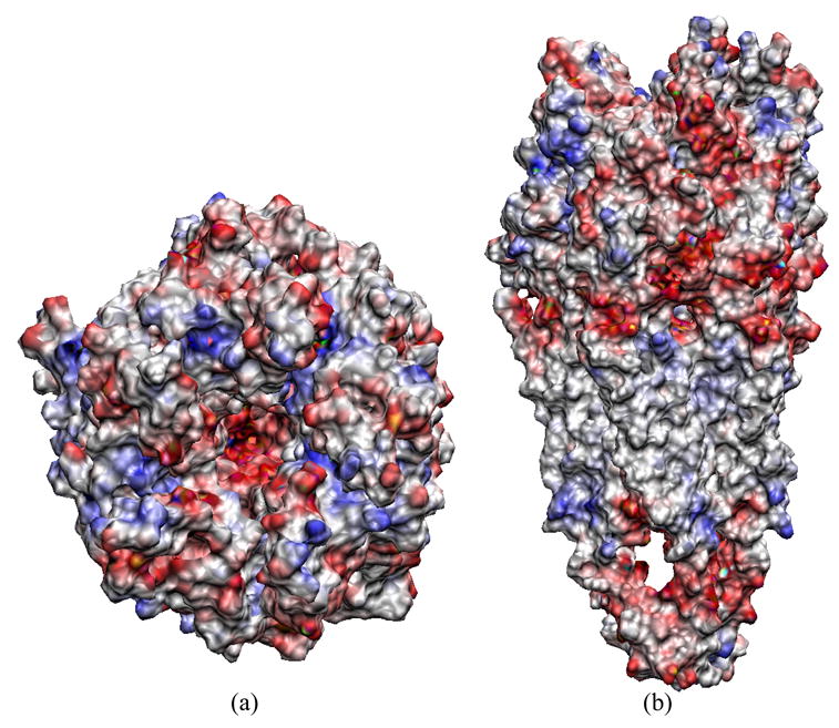
The BEM calculation is performed on a two-domain system if two molecules move away and two separate meshes are generated or on a single domain system if two molecules are close enough to ’merge’ and only a single mesh generated. For intermolecular electrostatics, the present BEM method provides the full PB interaction energy that takes into account both the desolvation and mutual polarization contributions from the two molecules. Figure 7a shows the electrostatic potentials mapped on the molecular surfaces of Sso7d and DNA at a separation of 10 Å. The potential surfaces exhibit good electrostatic complementarity at the binding interface. Electrostatic attraction governs the intermolecular interaction at distances larger than ~ 5Å (Figure 7b, black line). Nevertheless, the electrostatic interaction becomes repulsive at close distances. A closer inspection of the complex structure suggests that a significant component of the binding free energy is due to the non-electrostatic interactions, made in large part by the interfacial hydrophobic residues.³⁷ The origin of the large unfavorable electrostatic interaction at close separations can be attributed to the electrostatic desolvation, an effect due to the unfavorable exclusion of the high dielectric solvent around one protein when the other one approaches. As a comparison, we also calculate the screened Coulomb interactions by summing up all the atomic pair contributions between Sso7d and DNA (see Figure 7b, red line). In this treatment, it is found that the interactions are all attractive across the whole separations. The values are close to the full BEM calculations at long distances, but the desolvation effects are obviously missed at close distances.

FIG. 7.

Electrostatics of Sso7d-DNA. (a) The surface potential map of Sso7d and DNA at separation of 10 Å. (b) The electrostatic interaction energies as functions of separation along the center-to-center unbinding direction. U_BEM is the full electrostatic interaction energy determined by our BEM, and U_Coulomb is the sum of all the atomic pair screened Coulomb interactions between Sso7d and DNA. The curves connect the calculation points (denoted by the diamond and star symbols) consecutively by fitting with cubic splines.

The electrostatic interaction characteristics displayed in Figure 7 are very similar to the acetylcholinesterase and fasciculinII complex system as has been demonstrated previously,³⁰ which also shows long-range attraction (>~ 5Å) and close-range repulsion. Another common observation of these two systems is that the electrostatic interactions start abruptly increasing from around 5Å. This is the distance where the water molecules between the two molecules are squeezed out, and the two molecules begin to collapse into a compact complex structure. At the same time, the generated molecular surface meshes of the two molecules also begin to merge into a single mesh. This implies that the interfacial non-polar interaction, hydrophobic packing, and possibly local conformational rearrangement upon binding take effects from around 5Å of association and become dominant binding forces in the final stage of complex formation.

4 Conclusions and Discussion

In this paper, an algorithm with an optimal computational complexity is presented by introducing the new version of FMM. This is combined with the well-conditioned BIE formula to solve the linearized PB electrostatics for systems of arbitrary numbers of biomolecules. This algorithm enhances our computational capability to treat large and complex biological systems. The method could possiblly be further developed for applications to dynamical simulations (Monte Carlo, Brownian dynamics, and all-atom molecular dynamics, etc) of proteins with full PB electrostatics. However, although the speed has been greatly improved, the dynamical computation for biosystems using the current algorithm still exceed the presently available computer capability. For a typical Brownian dynamics simulation with tens of millions of steps, the one-step PB solution needs to be completed within no more than a few tenths of a second to meet the total wall-clock time constraint. Based on this estimation, the present BEM solver is still about one order slower. Several techniques can be pursued to further increase the efficiency of the present algorithm. Using an adaptive FMM scheme can greatly decrease the memory usage because most “volume” boxes away from the boundary need not be stored and counted. Curvilinear boundary element methods can reduce the number of boundary elements by a few to several folds while achieving the similar calculation accuracy. Improvement on mesh generation can also help in dynamical simulation when changing boundaries occur due to conformational flexibility, because the surface meshes need to be regenerated on the fly. Finally, another way to increase the computational speed is to implement an efficient parallelization of the code. Very good scalability of parallelization is anticipated, due to the nature of both the BEM and FMM algorithms.

References

- 1.Abramowitz M, Stegun IA. Handbook of Mathematical Functions. Dover Publications; New York: 1965. [Google Scholar]
- 2.Altman M, Bardhan J, White J, Tidor B. An accurate surface formulation for biomolecule electrostatics in non-ionic solutions. Conf Proc IEEE Eng Med Biol Soc. 2005;7(NIL):7591–5. doi: 10.1109/IEMBS.2005.1616269. [DOI] [PubMed] [Google Scholar]
- 3.Altman MD, Bardhan JP, Tidor B, White JK. FFTSVD: a fast multiscale boundary-element method solver suitable for Bio-MEMS and biomolecule simulation. IEEE Trans Comput-Aided Des Integr Circuits Syst. 2006;25(2):274–284. [Google Scholar]
- 4.Appel AW. An efficient program for many-body simulations. SIAM J Sci Stat Comput. 1985;6:85–103. [Google Scholar]
- 5.Baker NA, Sept D, Joseph S, Holst MJ, McCammon JA. Electrostatics of nanosystems: application to microtubules and the ribosome. Proc Natl Acad Sci U S A. 2001;98(18):10037–10041. doi: 10.1073/pnas.181342398. [DOI] [PMC free article] [PubMed] [Google Scholar]
- 6.Barnes J, Hut P. A hierarchical o(n log n) force-calculation algorithm. Nature. 1986;324(4):446 – 449. [Google Scholar]
- 7.Bharadwaj R, Windemuth A, Sridharan S, Honig B, Nicholls A. The fast multipole boundary-element method for molecular electrostatics - an optimal approach for large systems. J Comput Chem. 1995;16(7):898–913. [Google Scholar]
- 8.Bordner AJ, Huber GA. Boundary element solution of the linear Poisson-Boltzmann equation and a multipole method for the rapid calculation of forces on macromolecules in solution. J Comput Chem. 2003;24(3):353–367. doi: 10.1002/jcc.10195. [DOI] [PubMed] [Google Scholar]
- 9.Boschitsch AH, Fenley MO, Olson WK. A fast adaptive multipole algorithm for calculating screened Coulomb (Yukawa) interactions. J Comput Phys. 1999;151(1):212–241. [Google Scholar]
- 10.Boschitsch AH, Fenley MO, Zhou HX. Fast boundary element method for the linear Poisson-Boltzmann equation. J Phys Chem B. 2002;106(10):2741–2754. [Google Scholar]
- 11.Capener CE, Kim HJ, Arinaminpathy Y, Sansom MSP. Ion channels: structural bioinformatics and modelling. Hum Mol Genet. 2002;11(20):2425–2433. doi: 10.1093/hmg/11.20.2425. [DOI] [PubMed] [Google Scholar]
- 12.Cornell WD, Cieplak P, Bayly CI, Gould IR, Merz KM, Ferguson DM, Spellmeyer DC, Fox T, Caldwell JW, Kollman PA. A 2nd generation force-field for the simulation of proteins, nucleic-acids, and organic-molecules. J Am Chem Soc. 1995;117(19):5179–5197. [Google Scholar]
- 13.Cortis CM, Friesner RA. An automatic three-dimensional finite element mesh generation system for the Poisson-Boltzmann equation. J Comput Chem. 1997;18(13):1570–1590. [Google Scholar]
- 14.Dacunha RD, Hopkins T. The parallel iterative methods (PIM) package for the solution of systems of linear equations on parallel computers. Appl Numer Math. 1995;19(1–2):33–50. [Google Scholar]
- 15.Darden T, York D, Pedersen L. Particle mesh ewald: An nlog(n) method for Ewald sums in large systems. J Chem Phys. 1993;98(12):10089–10092. [Google Scholar]
- 16.Davis ME, McCammon JA. Electrostatics in biomolecular structure and dynamics. Chem Rev. 1990;90(3):509–521. [Google Scholar]
- 17.Debye P, Huckel E. Zur theorie der elektrolyte. Phys Zeitschr. 1923;24:185–206. [Google Scholar]
- 18.Figueirido F, Levy RM, Zhou RH, Berne BJ. Large scale simulation of macromolecules in solution: combining the periodic fast multipole method with multiple time step integrators. J Chem Phys. 1997;106(23):9835–9849. [Google Scholar]
- 19.Gilson MK, Rashin A, Fine R, Honig B. On the calculation of electrostatic interactions in proteins. J Mol Biol. 1985;184(3):503–516. doi: 10.1016/0022-2836(85)90297-9. [DOI] [PubMed] [Google Scholar]
- 20.Greengard L, Rokhlin V. A fast algorithm for particle simulations. J Comput Phys. 1987;73(2):325–348. [Google Scholar]
- 21.Greengard L, Rokhlin V. A new version of the fast multipole method for the laplace equation in three dimensions. Acta Numerica. 1997;6:229–269. [Google Scholar]
- 22.Greengard LF, Huang JF. A new version of the fast multipole method for screened coulomb interactions in three dimensions. J Comput Phys. 2002;180(2):642–658. [Google Scholar]
- 23.Holst M, Baker N, Wang F. Adaptive multilevel finite element solution of the Poisson-Boltzmann equation i. algorithms and examples. J Comput Chem. 2000;21(15):1319–1342. [Google Scholar]
- 24.Juffer AH, Botta EFF, Vankeulen BAM, Vanderploeg A, Berendsen HJC. The electric-potential of a macromolecule in a solvent - a fundamental approach. J Comput Phys. 1991;97(1):144–171. [Google Scholar]
- 25.Kapur S, Long DE. IES3: Efficient electrostatic and electromagnetic simulation. IEEE Comput Sci Eng. 1998;5(4):60–67. [Google Scholar]
- 26.Kirkwood JG. On the theory of strong electrolyte solutions. J Chem Phys. 1934;2:767–781. [Google Scholar]
- 27.Klapper I, Hagstrom R, Fine R, Sharp K, Honig B. Focusing of electric fields in the active site of Cu-Zn superoxide dismutase: effects of ionic strength and amino-acid modification. Proteins. 1986;1(1):47–59. doi: 10.1002/prot.340010109. [DOI] [PubMed] [Google Scholar]
- 28.Kuo SS, Altman MD, Bardhan JP, Tidor B, White JK. Fast methods for simulation of biomolecule electrostatics. ICCAD ’02: Proceedings of the 2002 IEEE/ACM international conference on Computer-aided design, ACM Press; New York, NY, USA. 2002. [Google Scholar]
- 29.Liang J, Subramaniam S. Computation of molecular electrostatics with boundary element methods. Biophys J. 1997;73(4):1830–1841. doi: 10.1016/S0006-3495(97)78213-4. [DOI] [PMC free article] [PubMed] [Google Scholar]
- 30.Lu BZ, Cheng XL, Huang JF, McCammon JA. Order N algorithm for computation of electrostatic interactions in biomolecular systems. Proc Natl Acad Sci U S A. 2006;103(51):19314–19319. doi: 10.1073/pnas.0605166103. [DOI] [PMC free article] [PubMed] [Google Scholar]
- 31.Lu BZ, McCammon JA. Improved boundary element methods for Poisson-Boltzmann electrostatic potential and force calculations. J Chem Theory Comput. 2007;3(3):1134–1142. doi: 10.1021/ct700001x. [DOI] [PubMed] [Google Scholar]
- 32.Lu BZ, Zhang DQ, McCammon JA. Computation of electrostatic forces between solvated molecules determined by the poisson-boltzmann equation using a boundary element method. J Chem Phys. 2005;122(21):214102. doi: 10.1063/1.1924448. [DOI] [PubMed] [Google Scholar]
- 33.Ong ET, Lee KH, Lim KM. A fast algorithm for three-dimensional electrostatics analysis: fast fourier transform on multipoles (FFTM) Int J Numer Methods Eng. 2004;61(5):633–656. [Google Scholar]
- 34.Ong ET, Lim KM, Lee KH, Lee HP. A fast algorithm for three-dimensional potential fields calculation: fast Fourier transform on multipoles. J Comput Phys. 2003;192(1):244–261. [Google Scholar]
- 35.Phillips JR, White JK. A precorrected-FFT method for electrostatic analysis of complicated 3-D structures. IEEE Trans Comput-Aided Des Integr Circuits Syst. 1997;16(10):1059–1072. [Google Scholar]
- 36.Richards FM. Areas, volumes, packing, and protein-structure. Annu Rev Biophys Bioeng. 1977;6:151–176. doi: 10.1146/annurev.bb.06.060177.001055. [DOI] [PubMed] [Google Scholar]
- 37.Robinson H, Gao YG, Mccrary BS, Edmondson SP, Shriver JW, Wang AHJ. The hyperthermophile chromosomal protein Sac7d sharply kinks DNA. Nature. 1998;392(6672):202–205. doi: 10.1038/32455. [DOI] [PubMed] [Google Scholar]
- 38.Rokhlin V. Solution of acoustic scattering problems by means of second kind integral equations. Wave Motion. 1983;5(3):257–272. [Google Scholar]
- 39.Sanner MF, Olson AJ, Spehner JC. Reduced surface: an efficient way to compute molecular surfaces. Biopolymers. 1996;38(3):305–320. doi: 10.1002/(SICI)1097-0282(199603)38:3%3C305::AID-BIP4%3E3.0.CO;2-Y. [DOI] [PubMed] [Google Scholar]
- 40.Sharp KA, Honig B. Electrostatic interactions in macromolecules - theory and applications. Annu Rev Biophys Biophys Chem. 1990;19:301–332. doi: 10.1146/annurev.bb.19.060190.001505. [DOI] [PubMed] [Google Scholar]
- 41.Shi W, Liu J, Kakani N, Yu T. A fast hierarchical algorithm for 3-D capacitance extraction. DAC ’98: Proceedings of the 35th annual conference on Design automation, ACM Press; New York, NY, USA. 1998. [Google Scholar]
- 42.Tanaka M, Sladek V, Sladek J. Regularization techniques applied to boundary element method. AMSE Appl Mech Rev. 1994;47:457–499. [Google Scholar]
- 43.Tausch J, White J. A multiscale method for fast capacitance extraction. DAC ’99: Proceedings of the 36th ACM/IEEE conference on Design automation, ACM Press; New York, NY, USA. 1999. [Google Scholar]
- 44.Totrov M, Abagyan R. Rapid boundary element solvation electrostatics calculations in folding simulations: successful folding of a 23-residue peptide. Biopolymers. 2001;60(2):124–133. doi: 10.1002/1097-0282(2001)60:2<124::AID-BIP1008>3.0.CO;2-S. [DOI] [PubMed] [Google Scholar]
- 45.Unwin N. Refined structure of the nicotinic acetylcholine receptor at 4 angstrom resolution. J Mol Biol. 2005;346(4):967–989. doi: 10.1016/j.jmb.2004.12.031. [DOI] [PubMed] [Google Scholar]
- 46.Warwicker J, Watson HC. Calculation of the electric-potential in the active-site cleft due to alpha-helix dipoles. J Mol Biol. 1982;157(4):671–679. doi: 10.1016/0022-2836(82)90505-8. [DOI] [PubMed] [Google Scholar]
- 47.Xin W, Juffer AH. A boundary element formulation of protein electrostatics with explicit ions. J Comput Phys. 2007;223:416–435. [Google Scholar]
- 48.Zauhar RJ, Morgan RS. A new method for computing the macromolecular electric-potential. J Mol Biol. 1985;186(4):815–820. doi: 10.1016/0022-2836(85)90399-7. [DOI] [PubMed] [Google Scholar]
- 49.Zauhar RJ, Varnek A. A fast and space-efficient boundary element method for computing electrostatic and hydration effects in large molecules. J Comput Chem. 1996;17(7):864–877. [Google Scholar]