Computing a family of skeletons of volumetric models for shape description

Abstract

Skeletons are important shape descriptors in object representation and recognition. Typically, skeletons of volumetric models are computed using iterative thinning. However, traditional thinning methods often generate skeletons with complex structures that are unsuitable for shape description, and appropriate pruning methods are lacking. In this paper, we present a new method for computing skeletons of volumetric models by alternating thinning and a novel skeleton pruning routine. Our method creates a family of skeletons parameterized by two user-specified numbers that determine respectively the size of curve and surface features on the skeleton. As demonstrated on both real-world models and protein images in bio-medical research, our method generates skeletons with simple and meaningful structures that are particularly suitable for describing cylindrical and plate-like shapes.

1 Introduction

Representing and understanding shapes play central roles in many of today’s graphics and vision applications. These applications often benefit from some form of shape descriptors, one of which is known as skeletons. A skeleton is a compact, medial structure that lies within a solid object [8]. A skeleton of a 2D object consists of 1D (e.g., curve) elements, whereas the skeleton of a 3D object may consist of both 1D and 2D (e.g., surface) elements. A skeleton that captures essential topology and shape information of the object in a simple form is extremely useful in solving various problems such as character recognition, 3D model matching and retrieval, and medical image analysis.

Here we consider computing skeletons of a 3D object consisting of lattice points in a binary volume. While there has been numerous work on 2D skeletonization (see an excellent survey in [15]), methods for computing 3D skeletons are relatively scarce. Skeletonizing volumetric objects often utilizes a thinning process that iteratively removes deletable object points until a thin, skeletal structure is left. To preserve the object’s topology during thinning, deletable points must be simple [16,24,5] in that their removal does not invoke topology change. In addition, to prevent shrinking of curves or surfaces that may carry the object’s shape information, various types of curve-end points or surface-end points [16,30,13,7,6,18] can be identified and preserved during thinning. Thinning methods can also be classified as sequential [25], meaning deletable points are identified and removed one after another, or parallel (see review in [22]), meaning all deletable points are collected first and removed in a batch.

Unfortunately, the skeletons computed by thinning methods often exhibit a complex structure. For example, Figure 1 (b) shows the result of the parallel thinning method of Bertrand [6] on the chair model in (a). Note in particular that the spurious surface branches do not provide meaningful information about the original object, and the chair legs can be represented in a simpler and more descriptive manner by curves instead of surfaces. Although numerous pruning methods exist for 2D skeletons [3,26], for skeletons of 3D point-set and polygonal models [21,2,1,11,12,29,27], or for removing only curve branches from skeletons of volumetric models [19,28], pruning both redundant curve and surface features from skeletons resulted from thinning remains an open problem.

Fig. 1.

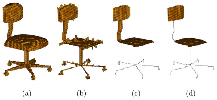
A volumetric chair object (a), the skeleton computed using the parallel thinning method of Bertrand [6] (b), and two skeletons computed using our method with parameters d₁ = 20, d₂ = 4 (c) and d₁ = 20, d₂ = 7 (see explanations in Section 3.2).

We present a new method for computing simple, topology-preserving and shape-depicting skeletons of a volumetric model. The core of this method is a simple and efficient pruning algorithm capable of removing redundant curve features as well as surface features from a skeleton computed by thinning. Given a volumetric object, pruning and thinning are alternated to produce the final skeleton. Governed by two user-specified pruning parameters, our method allows flexible control over the size of skeleton curves and surfaces, and varying the parameters produces a family of skeletons. Figure 1 (c,d) give two example skeletons computed using our method with different pruning parameters.

An interesting application that we shall explore is the use of our computed skeletons in describing cylindrical and plate-like shapes. Models composed of these two shapes are not only common around us, such as chairs and tables, but also within us, such as the bone matrix [23,9] and the protein structure (which we will see in Section 4). Previous approaches for identifying these two types of shapes involve complicated classification of points on an unpruned skeleton resulted from thinning [23,9], which can be highly sensitive to the complexity of the skeleton. Using appropriate pruning parameters, our method yields descriptive skeletons whose curves and surfaces correspond well to the cylindrical and plate-like parts of the object, as seen in Figure 1 (c,d), thus allowing easy identification of these shape components.

In Section 2, we review related concepts in digital topology, and introduce a new geometric characterization of discrete curves and surfaces that lay the theoretical foundation of our method. The details of the thinning and pruning algorithms are described in Section 3, and experimental results are shown in Section 4. In addition, we present in Section 4 a bio-medical application and demonstrate how the computed skeletons can be useful for identifying structural components of a protein model from low-resolution images.

2 Digital topology and discrete geometry

2.1 Simple points

We consider a volumetric model as a uniform 3D lattice consisting of object points V and background points V̄. For topology analysis, we classify the 3 × 3 × 3 neighborhood of each lattice point x into three (overlapping) sets, N₆(x), N₁₈(x) and N₂₆(x), each consisting of points (other than x) that share a common grid edge, face or cell with x. The three sets are illustrated in Figure 2 (a). In addition, we denote N_k(x, V) = N_k (x) ∩ V.

Fig. 2.

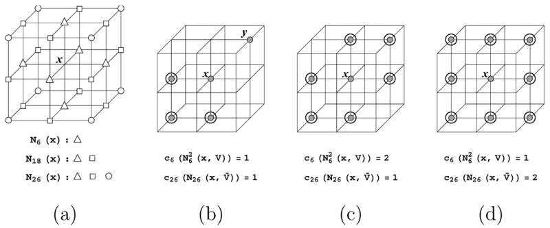
The 3 × 3 × 3 neighborhood of a lattice point x with the sets N₆(x), N₁₈(x), N₂₆(x) labelled (a), and three example configurations of object points in this neighborhood (b,c,d), where N₂₆(x, V) are filled dots (N₂₆(x, V̄) are unmarked lattice points) and $N_6^2(x,V)$ are highlighted.

The topology of the object V is determined by the connectivity of points in V. We regard two points x, y as k-connected if y ∈ N_k (x) for k = 6, 18, 26. In this paper we assume that the object points are 6-connected and the background points are 26-connected, so that the topology of the set V agrees with that of the iso-surface of the whole volume generated by mainstream contouring techniques, such as the Marching Cubes method and its variants [17,20]. In order to maintain topology of V during skeletonization, we follow the result of Bertrand [5] to determine if a point x ∈ V is simple with respect to V, that is, if V \ {x} preserves the topology of V:

Proposition 1 (Bertrand)

Let s(V) denote the set of simple points of V, then x ∈ s(V) if and only if $c_6(N_6^2(x,V)=1$ and c₂₆(N₂₆(x, V̄)) = 1. Here c_k(X) computes the number of k-connected components in point set X, and

$$N_6^2(x,V)=N_6(x,V)\cup \underset{y\in N_6(x,V)}{\cup }M(x,y,V),$$

where M (x, y, V) = N₁₈(x, V) ∩ N₆(y, V).

In words, $N_6^2(x,V)$ is the set of points in N₁₈(x, V) that are either 6-connected to x or to a 6-connected object neighbor of x. In Figure 2 (b,c,d), we show three example configurations of object points in the neighborhood of x, where the set $N_6^2(x,V)$ is highlighted. Observe in Figure 2 (b) that object point y ∈ N₁₈(x, V) does not belong to $N_6^2(x,V)$. By Proposition 1, x is a simple point in configuration (b) but not in configuration (c) or (d).

2.2 Discrete curves and surfaces

A curve in an object V is a connected collection of object edges, each composed of two 6-connected object points, and a surface in V is a connected collection of object faces, each composed of four 18-connected object points. In Figure 3, edges are shown as dark lines and faces as orange polygons.

Fig. 3.

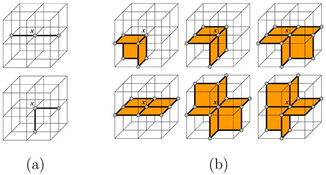
Examples of locally 1-manifold subsets of N₆(x, V) (a) and locally 2-manifold subsets of N₁₈(x, V) (b).

Knowledge of curves and surfaces is critical as they are the components of a skeleton that carry shape information of the object. To prevent loss of such information during thinning, it is important to avoid shrinking of the curves and surfaces. While various definitions of curve-end and surface-end points have been proposed in previous work [16,30,13,7,6,18], few are designed for 6-connected objects (except in [6]).

In our new definition, a set S ⊆ N₆(x, V) is called locally 1-manifold if S ∪ {x} forms two edges containing x, and S ∈ N₁₈(x, V) is called locally 2-manifold if S ∪ {x} forms a ring of faces containing x that are topologically equivalent to a disk. Figure 3 enumerates all rotationally distinct cases of local manifolds. A point x ∈ V is therefore a curve-end (or surface-end) point if N₆(x, V) (or N₁₈(x, V)) does not contain any locally 1-manifold (or 2-manifold) subset. Intuitively, there exists no curve that passes through a curve-end point, and no surface that completely surrounds a surface-end point. Both curve-end and surface-end points can be efficiently identified as follows:

Proposition 2

Let ∂_m(V) denote the set of curve-end (m = 1) or surface-end (m = 2) points of an object V, for any x ∈ V we have

1. x ∈ ∂₁(V) if and only if #N₆(x, V) < 2.

2. x ∈ ∂₂(V) if and only if

$$\sum _{y\in N_6(x,V)}\#M(x,y,V)-\#N_6^2(x,V)-c_6(N_6^2(x,V))=0$$ (1)

Here # computes set cardinality and $N_6^2(x,V)$, M(x, y, V) are defined in Proposition 1.

Proof

1. By definition, x is not a curve-end point if N₆(x, V) contains more than two points, which form at least two edges with x.

2. First we observe that the quantity Σ_{y ∈ N6(x, V)} #M(x, y, V) equals to the number of edges formed by points in the set $N_6^2(x,V)$. Consider the graph formed by the points and edges in $N_6^2(x,V)$, the left-hand side of Equation 1 in fact computes the number of closed rings of edges in the graph. Furthermore, each such ring is a locally 2-manifold subset of N₁₈(x, V). Hence x ∈ ∂₂(V) if and only if $N_6^2(x,V)$ does not contain any rings. □

In addition to curve-end and surface-end points, we are also interested in the local neighborhood of each interior point on a curve or surface. An object point y is called a curve-neighbor (or surface-neighbor) of x if y lies in a locally 1-manifold (or 2-manifold) subset of N₆(x, V) (or N₁₈(x, V)). Like end points, we present an explicit characterization of neighbor points:

Proposition 3

Let ω_m(x, V) denote the set of curve-neighbor (m = 1) or surface-neighbor (m = 2) points of x ∈ V, for any y ∈ V we have

1. y ∈ ω₁(x, V) if and only if y ∈ N₆(x, V) and #N₆(x, V) ≥ 2.

2. y ∈ ω₂(x, V) if and only if y ∈ N₁₈(x, V) and r(x, V) > r(x, V \ {y}), where r(x, V) is defined as the left-hand side of Equation 1.

Proof

1. By definition, y is a curve-neighbor of x only if y lies in a locally 1-manifold subset of N₆(x, V), which requires both the existence of such a subset, i.e. #N₆(x, V) ≥ 2, and that y ∈ N₆(x, V).

2. From the proof of Proposition 2, we know that r(x, V) counts the number of possible locally 2-manifold subsets of N₁₈(x, V). y lies in a locally manifold subset of N₁₈(x, V) if and only if removing y from V reduces the number of manifold subsets.

3 The algorithms

Our algorithm computes the skeleton of a volumetric model by alternating two operations: thinning and skeleton pruning. For thinning, we adopt the standard iterative paradigm while incorporating our new end-points definition for shape preservation. For pruning, we introduce a simple and effective morphological procedure on discrete curves and surfaces. The algorithms of thinning and pruning are discussed separately, and the complete method is presented next.

3.1 Iterative thinning

Thinning begins with a volumetric object V with boundary points ∂(V). Assuming 6-connectivity of the object (as explained in Section 2.1), the boundary is defined as

$$\partial (V)=\{x\mid x\in V\hspace{0.17em}\text{and}\hspace{0.17em}{N}_6(x,\overline{V})\ne \varnothing \}$$

Thinning removes each boundary point from V except for critical points, whose removal will alter the topology of V or result in loss of shape information. Following the discussion in the previous section, a critical point x can be either a non-simple point, a curve-end point or a surface-end point. We can write this definition of a critical point as a boolean expression:

$${\mathit{IsCritical}}_m(x,V)=x\notin s(V)\hspace{0.17em}\text{or\hspace{0.17em}}x\hspace{0.17em}\in \hspace{0.17em}{\partial }_m(V)$$

Here, the subscript m = 0, 1, 2 determines whether discrete surfaces (m = 2) or curves (m = 1) in addition to the topology of V are to be preserved during thinning, or only topology information will be preserved (m = 0, where we let ∂₀(V) = ∅).

Note that based on the above definition, a curve-end or surface-end point that forms a small surface bump can be identified as critical points, such as those shown in Figure 4 (a,c) (end-points are drawn as triangles). These bumps are often resulted from discretizing a smooth surface. To distinguish discretization artifacts from shape features, in practice, we add an additional restriction such that a curve-end (or surface-end) point is critical only if it is contained in an edge (or face) that contains only boundary points. As a result, only curve-end and surface-end points in Figure 4 (b,d) are considered critical.

Fig. 4.

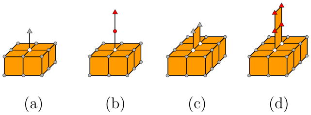
Defining critical points: A curve-end or surface-end point (shown as triangles) is critical (colored red) only if it is shared by an edge or face that does not contain any non-boundary points (colored white).

The pseudo-code of thinning is shown in Figure 5. Thinning is performed iteratively. At each iteration, all boundary points are placed in a queue Q and are visited and removed sequentially. The program Thin_m takes an extra parameter S, which is a subset of V that will be “protected” during thinning, i.e., no point of S will be removed from V. The use of S will become clear when the complete method is presented in Section 3.3.

Fig. 5.

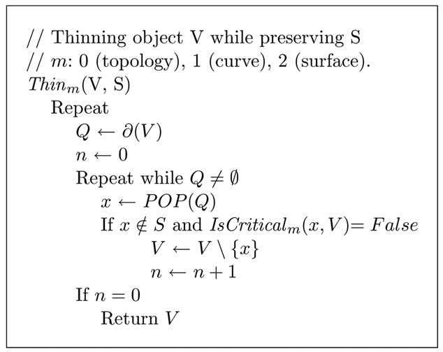
Pseudo code for iterative thinning.

Note that the sequence in which boundary points are ordered (and visited) in the queue Q at each iteration of Thin_m affects the complexity of the resulting skeleton. In particular, an arbitrary ordering could result in a large number of boundary points being classified as critical points, and hence produce an excessive amount of noisy features on the skeleton. In the example of Figure 6, applying Thin₁ and Thin₂ on a regular array of object points in (a) yields unnecessarily complex skeletons in (b,c) when elements in Q are visited in a random order. In our implementation, we found that ordering (and visiting) boundary points x in Q in the ascending order of #N₆(x, V) significantly reduces such complexity, as shown in Figure 6 (d,e). Intuitively, such ordering ensures points that are at the “corner” of the object are removed earlier than those in the “middle” of the object boundary.

Fig. 6.

Thinning an object (a) by Thin₁ (b,d) and Thin₂ (c,e) where boundary points x in the queue Q are visited in a random order (b,c) or in the ascending order of #N₆(x, V) (d,e).

For convenience, we refer to program Thin_m as surface thinning (m = 2), curve thinning (m = 1), or topology thinning (m = 0). Figure 7 shows the result of thinning on three primitive shapes: a sphere, a cylinder and a plate. Observe in particular that surface thinning generates large surfaces for plate-like shapes, while curve thinning results in long curves for cylindrical shapes.

Fig. 7.

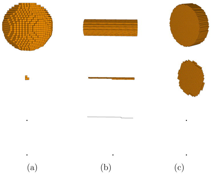
Volumetric objects (top row) and their skeletons after surface thinning (second row), curve thinning (third row) and topology thinning (bottom row). The black dot represents a single skeleton point.

3.2 Skeleton pruning

Pruning is the process of removing redundant curve or surface features from a skeleton object. Examples of redundant features that we wish to remove include short curve branches, small surface branches, jagged surface borders and narrow surface bands. Our algorithm extends two morphological operators, namely erosion and dilation, which are often coupled (known as opening) in digital imaging to remove small and narrow image artifacts and to smoothen jagged object borders. The operators are adapted here to remove excessive features on discrete curves and surfaces.

Like thinning, pruning can be applied to any collection of object points. Given an object V and a super-set V′⊃V, our definition of erosion and dilation is based on end-points and neighbor-points introduced in Section 2.2:

$$\begin{array}{l}\mathit{Erod}{e}_m(V)=V\backslash {\partial }_m(V)\\ \mathit{Dilat}{e}_m(V,V^{\prime })=V\cup {\cup }_{x\in {\partial }_m(V)}{\omega }_m(x,V^{\prime })\end{array}$$

where m = 1 or 2, ∂₁(V), ∂₂(V) are curve-end and surface-end points, and ω₁(x, V), ω₂(x, V) are curve-neighbor and surface-neighbor points. In words, erosion retracts V along its curve (m = 1) or surface (m = 2) border, while dilation expands V towards a larger set V′ by growing manifold neighborhoods from the curve (m = 1) or surface (m = 2) border of V. Note that unlike thinning, erosion and dilation are topology-altering. Figure 8 shows an example of applying two rounds of surface erosion (b,c) followed by two rounds of surface dilation (d,e). The object after i rounds of erosion (i = 0, 1) is used as the super-set V′ for the (2 − i)th round of dilation.

Fig. 8.

An input object (a), the result of applying two rounds of surface erosion (b,c), followed by two rounds of surface dilation (d,e). Eroded or dilated points at each round are highlighted.

In the example shown in Figure 8 for m = 2, we observe that the combination of Erode₂ and Dilate₂ has the effect of removing small, narrow surface features and smoothing borders. We couple the two operators to form pruning, which is recursively defined as

$${\mathit{Prune}}_m(V,d_m)=\mathit{Dilat}{e}_m({\mathit{Prune}}_m(\mathit{Erod}{e}_m(V),d_m-1),V).$$

where d_m ≥ 0 is the pruning parameter, and Prune_m(V, 0) = V.

The pseudo-code of pruning is provided in Figure 9. Pruning is performed recursively. At each recursion level, the eroded object V \ ∂ (V) is first passed to the next level. Given the pruned object S returned from the recursive call, the boundary points of S are then placed in a queue Q and processed sequentially for dilation. For each point x ∈ Q, dilation searches within the N₆(x, V) for curve-neighbor points (or the N₁₈(x, V) for surface-neighbor points) and adds them to S. Note that, instead of storing multiple copies of V during recursion, an integer value d[x] can be computed and stored at each point x ∈ V keeping track of recursion levels. Initially, all d[x] are initialized as ∞. During recursion, d[x] is first set to the level of recursion where x is eroded, and later reset to ∞ when it is dilated.

Fig. 9.

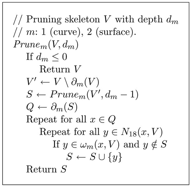
Pseudo code for skeleton pruning.

Like thinning, we refer to Prune₁(V, d₁) as curve pruning and Prune₂(V, d₂) as surface pruning. Examples of pruning can be found as part of Figure 10 on the right, where surface pruning (top) and curve pruning (bottom) are applied with various parameters. Observe that larger values of d₁ remove longer curve branches, while larger values of d₂ remove wider surface bands and produce smoother surface borders. An important feature of our pruning method is that it does not shrink major curves or surfaces as a result of removing noises.

Fig. 10.

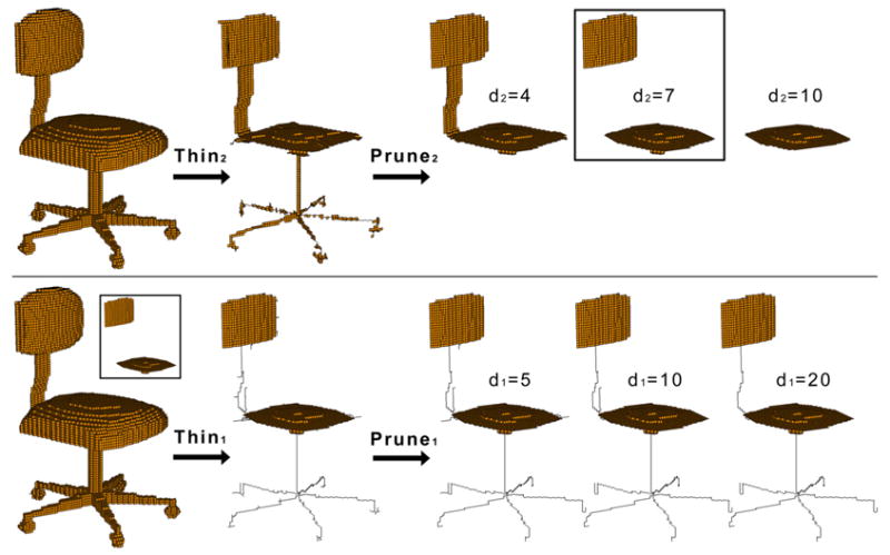
Stage 1 (top) and 2 (bottom) in generating a skeleton. In the second stage, d₂ = 7 is used as input while several values of d₁ are tested. Note that in the second stage, curve thinning preserves the surfaces (shown in the insert) computed by the first stage.

3.3 The complete method

We have presented two independent algorithms so far: a thinning operation that preserves the topology of the object yet may result in redundant features on the skeleton, and a pruning operation that removes excessive curve or surface features from a skeletal object yet may alter its topology. To create a skeleton that is both topology-preserving and composed of meaningful features, we alternate thinning and pruning. Given an initial object V and pruning parameters d₁, d₂, we compute the final skeleton S in three stages:

Stage 1

Extract major surface features by surface thinning followed by surface pruning (Figure 10 top):

$$S\leftarrow {\mathit{Prune}}_2(\mathit{Thi}{n}_2(V,\varnothing ),d_2).$$.

Stage 2

Extract major curve features by curve thinning followed by curve pruning (Figure 10 bottom):

$$S\leftarrow {\mathit{Prune}}_1(\mathit{Thi}{n}_1(V,S),d_1).$$.

Stage 3

Ensure topology preservation through topology thinning:

$$S\leftarrow \mathit{Thi}{n}_0(V,S).$$

Observe that our method follows the alternating sequence of (surface) thinning, (surface) pruning, (curve) thinning, (curve) pruning, and (topology) thinning. Note that thinning in each stage is applied to the original object V. Except for stage 1, thinning in both stages 2 and 3 also preserve major surfaces and curves computed in the previous stage (through the use of the argument S in program Thin_m(V, S)). The final stage is necessary to ensure a topology-preserving skeleton, as pruning may alter the topology of the object V.

The combination of thinning and pruning allows a whole spectrum of skeletons being generated by changing the two parameters d₁, d₂. For example, we can reproduce the result of directly applying surface thinning (Thin₂(V, ∅)), curve thinning (Thin₁(V, ∅)) and topology thinning (Thin₀(V, ∅)) using parameters {d₁, d₂} = {0, 0}, {∞, 0} and {∞, ∞}. More importantly, as observed in Figure 10, reasonable choices of d₁, d₂ would yield skeletons whose curves and surfaces correspond well to cylindrical and plate-like shapes of the original object. In addition, varying the parameters allow the user to adjust the differentiation between these two shape types (Figure 1 is such an example).

4 Results

We demonstrate our skeletonization method on several artificial and scanned models, as shown in Figure 11 and 12. Each model is originally represented in polygonal formats and converted into volumetric forms using the PolyMender software [14]. Observe that our skeleton accurately captures the three structural components of the goblet, which is composed of 2 plates and 1 cylinder.

Fig. 11.

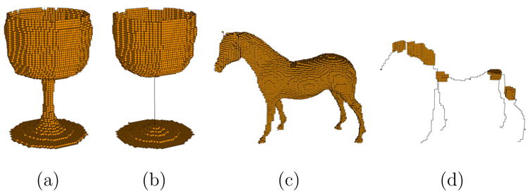
A goblet (a) and a horse (c) with their skeletons (b,d). Pruning parameters d₁ = 20 and d₂ = 3 are used in both examples.

Fig. 12.

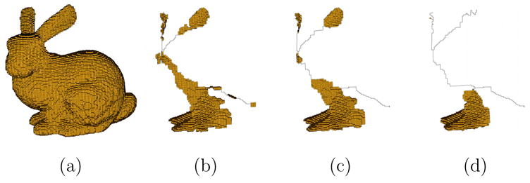
A bunny model (a) and its skeletons with parameters {d₁, d₂} at {50, 2} (b), {50, 4} (c) and {50, 10} (d).

Although the horse and the bunny do not consist of obvious cylinders and plates, the skeletons still provide a descriptive view of its overall shape as well as the difference among local shapes. Note from Figure 12 that varying the pruning parameter gives multiple choices of skeletons that may be useful in different applications.

We have also applied our method in the bio-medical setting for identifying β-sheet elements from low-resolution protein images. Figure 13 (a) shows protein density models reconstructed from cryo-electron microscopy (cryo-EM). Unlike X-ray crystallography, cryo-EM is capable of imaging large molecular assemblies in nearly native states [10]. However, the drawback of cryo-EM is that the reconstructed model has a much lower resolution (typically 6 to 10 Å) than that of X-ray (less than 3 Å), and resolving atomic details is not possible. Nevertheless, secondary structures of the protein, such as α-helices, β-sheets and loops, are discernable at this resolution and can be recognized as cylinders (loops and α-helices) and curved plates (β-sheets).

Fig. 13.

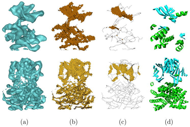
The iso-surface models of proteins IRK and 1BVP (a), the skeletons computed by [6] (b), the skeletons computed using our method with d₁ = d₂ = 3 (c), and the actual structures of these proteins determined by X-ray crystallography (d), where blue stripes denote β-sheets and green spirals denote α-helices. Observe that the skeleton surfaces computed by our algorithm correspond well to the actual β-sheets in the protein structure.

We applied our method to cryo-EM models, and the resulted skeletons (shown in Figure 13 (c)) differentiate cylindrical and plate-like shapes as skeleton curves and surfaces. In contrast, applying Bertrand’s parallel technique [6] yields far more surface components on the skeleton than our method, as shown in Figure 13 (b), making it impossible to differentiate plate-like and cylindrical shapes. The differentiation provided by our method allows β-sheets to be identified as skeleton surfaces in an automatic manner. We validate our result by comparing our skeleton with the actual protein structure revealed by X-ray experiments, shown in Figure 13 (d), where β-sheets are drawn as parallel blue arrows (each arrow representing a strand in the sheet). Note that the majority of the β-sheets have been correctly identified as skeleton surfaces. However, a small number of β-sheets (mostly consisting of only 2 strands) do not exhibit a plate-like shape in the cryo-EM models and hence were not identified by the skeleton. Nonetheless, combining the skeleton structure with cryo-EM density information, we have been able to identify both α-helices and β-sheets from cryo-EM models in a reliable manner [4].

In contrast to previous skeletonization algorithms that typically involve one pass of thinning, our method involves three passes of thinning and two passes of pruning. As a result, our method runs slower than most thinning methods, as shown in Table 1, yet still at a reasonable speed. All experiments were run on a PC with Pentium 4 CPU at 1.7GHz and 512MB memory. The timings are broken down into each thinning and pruning pass and are compared with the parallel thinning method of Bertrand [6].

Table 1.

Performance of skeletonization for the examples in this paper. The timings are recorded in seconds, and are broken down into thinning and pruning operations in each stage, see Section 3.3.

Model	Grid Size	Object Points	Stage 1 Thin	Stage 1 Prune	Stage 2 Thin	Stage 2 Prune	Stage 3 Thin	Total Time	Bertrand [6]
Goblet	64	15911	0.79	0.08	0.24	0.02	0.15	1.28	0.15
Chair	128	34920	1.28	0.28	1.04	0.19	0.65	3.44	1.21
Horse	128	54172	1.69	0.28	1.62	0.18	1	4.77	1.92
Bunny	128	214898	7.12	0.29	5.47	0.19	3.42	16.49	4.94
Protein 1IRK	128	10887	0.47	0.25	0.43	0.17	0.3	1.62	0.31
Protein 1BVP	128	24741	1.4	0.28	0.93	0.17	0.56	3.34	0.45

5 Conclusion and discussion

In this paper, we describe a method for computing a family of topology and shape preserving skeletons of a volumetric model. The method is compose of two algorithms: iterative thinning and skeleton pruning. Our method allows flexible control over the size of curves or surfaces on the resulting skeletons, which can be used for describing shapes of objects composed of cylindrical and plate-like regions.

One of the limitations of our method is that it requires two user-specified parameters for pruning skeleton curves and surfaces. One way to determine these parameters manually is by first generating a surface skeleton and letting the user identify the largest surface feature she wishes to remove from the skeleton, followed by computing a curve skeleton and identifying the longest curve branch that the user wishes to remove. In the future we would like to provide user with more convenient and direct means to specify these two pruning parameters. For example, one can imagine a user interface where the user may select representative tubes or plates on the model and the computer would determine the appropriate parameters automatically.

As other future directions of research, we are investigating more shape applications, such as segmentation, matching and recognition, using the skeleton generated by our method. In particular, we will explore the use of the skeletons of proteins in fast and accurate fold recognition and comparison, which is an important task demanded by researchers in structural biology.

References

- 1.Amenta N, Choi S, Kolluri RK. SMA ’01: Proceedings of the sixth ACM symposium on Solid modeling and applications. New York, NY, USA: ACM Press; 2001. The power crust; pp. 249–266. [Google Scholar]
- 2.Attali D, Montanvert A. Computing and simplifying 2d and 3d continuous skeletons. Comput Vis Image Underst. 1997;67(3):261–273. [Google Scholar]
- 3.Attali D, Sanniti di Baja G, Thiel E. Pruning discrete and semicontinuous skeletons. Lecture Notes in Computer Science, Image Analysis and Processing. 1995;974:488–493. [Google Scholar]
- 4.Baker ML, Ju T, Chiu W. Identification of secondary structure elements in intermediate resolution density maps. Structure. 2006 doi: 10.1016/j.str.2006.11.008. to appear. [DOI] [PMC free article] [PubMed] [Google Scholar]
- 5.Bertrand G. Simple points, topological numbers and geodesic neighborhoods in cubic grids. Pattern Recogn Lett. 1994;15(10):1003–1011. [Google Scholar]
- 6.Bertrand G. A parallel thinning algorithm for medial surfaces. Pattern Recogn Lett. 1995;16(9):979–986. [Google Scholar]
- 7.Bertrand G, Aktouf Z. Proceedings, SPIE Conference on Vision Geometry III. Vol. 2356. 1994. A 3d thinning algorithms using subfields; pp. 113–124. [Google Scholar]
- 8.Blum H. A transformation for extracting new descriptors of shape. In: Wathen-Dunn W, editor. Models for the Perception of Speech and Visual Forms. MIT Press; Amsterdam: 1967. pp. 362–380. [Google Scholar]
- 9.Bonnassie A, Peyrin F, Attali D. Shape description of three-dimensional images based on medial axis. ICIP. 2001;(3):931–934. doi: 10.1109/TSMCB.2003.814298. [DOI] [PubMed] [Google Scholar]
- 10.Chiu W, Baker M, Jiang W, Zhou Z. Deriving the folds of macromolecular complexes through electron cryomicroscopy and bioinformatics approaches. Curr Opin Struct Biol. 2002;2:263–269. doi: 10.1016/s0959-440x(02)00319-6. [DOI] [PubMed] [Google Scholar]
- 11.Dey TK, Zhao W. SMA ’02: Proceedings of the seventh ACM symposium on Solid modeling and applications. New York, NY, USA: ACM Press; 2002. Approximate medial axis as a voronoi subcomplex; pp. 356–366. [Google Scholar]
- 12.Foskey M, Lin MC, Manocha D. SM ’03: Proceedings of the eighth ACM symposium on Solid modeling and applications. New York, NY, USA: ACM Press; 2003. Efficient computation of a simplified medial axis; pp. 96–107. [Google Scholar]
- 13.Gong W, Bertrand G. A simple parallel 3d thinning algorithm. ICPR90. 1990:188–190. [Google Scholar]
- 14.Ju T. Robust repair of polygonal models. ACM Trans Graph. 2004;23(3):888–895. [Google Scholar]
- 15.Lam L, Lee S-W, Suen CY. Thinning methodologies-a comprehensive survey. IEEE Trans Pattern Anal Mach Intell. 1992;14(9):869–885. [Google Scholar]
- 16.Lee T-C, Kashyap RL, Chu C-N. Building skeleton models via 3-d medial surface/axis thinning algorithms. CVGIP: Graph Models Image Process. 1994;56(6):462–478. [Google Scholar]
- 17.Lorensen WE, Cline HE. Marching cubes: A high resolution 3d surface construction algorithm. SIGGRAPH ’87: Proceedings of the 14th annual conference on Computer graphics and interactive techniques; New York, NY, USA, ACM Press. 1987. pp. 163–169. [Google Scholar]
- 18.Ma CM. A 3d fully parallel thinning algorithm for generating medial faces. Pattern Recogn Lett. 1995;16(1):83–87. [Google Scholar]
- 19.Mekada Y, Toriwaki J. ICPR ’02: Proceedings of the 16 th International Conference on Pattern Recognition (ICPR’02) Volume 3. Washington, DC, USA: IEEE Computer Society; 2002. Anchor point thinning using a skeleton based on the euclidean distance transformation; pp. 923–926. [Google Scholar]
- 20.Natarajan BK. On generating topologically consistent isosurfaces from uniform samples. The Visual Computer. 1994;11(1):52–62. [Google Scholar]
- 21.Ogniewicz RL, Kübler O. Hierarchic Voronoi skeletons. Pattern Recognition. 1995;28(3):343–359. [Google Scholar]
- 22.Palágyi K, Kuba A. A parallel 3d 12-subiteration thinning algorithm. Graph Models Image Process. 1999;61(4):199–221. [Google Scholar]
- 23.Saha P, Gomberg B, Wehrli F. Three-dimensional digital topological characterization of cancellous bone architecture. IJIST. 2000;11(1):81–90. [Google Scholar]
- 24.Saha PK, Chaudhuri BB. Detection of 3-d simple points for topology preserving transformations with application to thinning. IEEE Trans Pattern Anal Mach Intell. 1994;16(10):1028–1032. [Google Scholar]
- 25.Saito T, Toriwaki J. A sequential thinning algorithm for three-dimensional digital pictures using the euclidean distance transformation. Proceedings of the 9th Scandinavian Conference on Image Analysis. 1995:507–516. [Google Scholar]
- 26.Shaked D, Bruckstein A. Pruning medial axes. Comput Vis Image Underst. 1998;69(2):156–169. [Google Scholar]
- 27.Sud A, Foskey M, Manocha D. SPM ’05: Proceedings of the 2005 ACM symposium on Solid and physical modeling. New York, NY, USA: ACM Press; 2005. Homotopy-preserving medial axis simplification; pp. 39–50. [Google Scholar]
- 28.Svensson S, Sanniti di Baja G. Simplifying curve skeletons in volume images. Comput Vis Image Underst. 2003;90(3):242–257. [Google Scholar]
- 29.Tam R, Heidrich W. Shape simplification based on the medial axis transform. IEEE Visualization. 2003:481–488. [Google Scholar]
- 30.Tsao YF, Fu KS. A parallel thinning algorithm for 3-d pictures. Comput Graphics Image Process. 1981;17:315–331. [Google Scholar]