

Abstract
Functional networks in the human brain have been investigated using electrophysiological methods (EEG/MEG, LFP, and MUA) and steady-state paradigms that apply periodic luminance or contrast modulation to drive cortical networks. We have used this approach with fMRI to characterize a cortical network driven by a checkerboard reversing at a fixed frequency. We found that the fMRI signals in voxels located in occipital cortex were increased by checkerboard reversal at frequencies ranging from 3 to 14 Hz. In contrast, the response of a cluster of voxels centered on basal medial frontal cortex depended strongly on the reversal frequency, consistently exhibiting a peak in the response for specific reversal frequencies between 3 and 5 Hz in each subject. The fMRI signals at the frontal voxels were positively correlated indicating a homogeneous cluster. Some of the occipital voxels were positively correlated to the frontal voxels apparently forming a large-scale functional network. Other occipital voxels were negatively correlated to the frontal voxels, suggesting a functionally distinct network. The results provide preliminary fMRI evidence that during visual stimulation, input frequency can be varied to engage different functional networks.
Keywords: Functional Connectivity, Functional Network, Frontal Cortex, Visual Cortex, SSVEP
Introduction
Functional brain networks that process sensory inputs can be investigated using steady-state paradigms that impose synchrony on populations of cortical neurons with a periodic stimulus. When human subjects are presented with sinusoidal contrast or luminance modulation of fixed frequency, which is usually superimposed on cognitive task-related images, steady state evoked potentials or magnetic fields can be easily detected by Fourier analysis of EEG or MEG signals (Regan, 1989; Narici et al., 1998; Tononi et al., 1998; Srinivasan et al., 1999; Srinivasan 2004; Silberstein, 1995; Silberstein et al., 2001; Chen et al., 2003). Steady-state responses are measured in the narrow (usually < 0.1 Hz) frequency band centered on the stimulus frequency. Since typical EEG/MEG artifacts, such as muscle potentials, have mostly broadband spectra, the the steady-state response has high signal to noise ratio in the narrow band surrounding the stimulation frequency and harmonics. This approach has had immense practical value in segregating stimulus related brain activity from both artifacts and spontaneous brain activity in cognitive and clinical studies.
Early human studies using EEG electrodes positioned over occipital cortex (Regan, 1977; Tyler et al., 1978; Regan, 1989), and local field potentials recorded within monkey visual cortex (Nakayama and Mackeben, 1982) demonstrated that steady-state responses recorded over visual cortex depend on the temporal frequency of visual input. The dependence of the magnitude of the steady-state response on the input frequency is characterized by local maxima in the response amplitude at the stimulation frequency in at least three different “resonance” bands. At occipital electrodes, these bands are roughly 7–10 Hz, 15–20 Hz, and 40–50 Hz, which Regan (1989) labeled as the low, middle, and high frequency region of the spectrum. Even at a single electrode site, individual subjects can show multiple response maxima within these bands. Studies of multi-unit activity (MUA) in the cat visual cortex with periodic stimulation have also shown a similar banded structure with peaks in the magnitude of the response at multiple stimulus frequencies in the 4–8 Hz, 16–30 Hz, and 30–50 Hz ranges (Rager and Singer, 1998). Steady-state responses in these different frequency bands show quite different sensitivities to physical stimulus parameters (color, spatial frequency, modulation depth, etc.) suggesting that flicker can entrain functionally distinct although spatially overlapping cortical networks at the cm scale of EEG (Regan, 1989). Because only a few electrodes over the occipital lobe were used in these studies, only minimal information was obtained about the spatial properties of SSVEPs in these different frequency bands.
The dynamics of steady-state responses to flickering stimuli have been studied with large (> 128) numbers of EEG electrodes and MEG sensors covering the whole scalp during binocular rivalry (Srinivasan et al., 1999; Srinivasan 2004; Srinivasan and Petrovic, 2006) selective attention (Chen et al., 2003; Ding et al., 2006), working memory (Silberstein et al., 2001) and other mental tasks (Silberstein et al., 2003; 2004). In these studies, steady state responses to a flickering visual stimulus have been recorded at many scalp locations beyond occipital channels. Channels over parietal, temporal, frontal, and prefrontal regions also exhibit SSVEP responses with amplitude, spatial distribution, and phase coherence depending on both the type of stimulus and the cognitive task.
The magnitude, phase, and spatial distribution of the SSVEP are extremely sensitive functions of the driving frequency, e.g., sensitive to 1 Hz changes in the theta (4–7 Hz) and alpha (8–12 Hz) bands (Nunez, 1995; Srinivasan, 2004; Ding et al., 2006; Srinivasan et al., 2006; Nunez and Srinivasan, 2006). Occipital SSVEPs can be recorded at most flicker frequencies. In contrast, SSVEPs are recorded over parietal, temporal, and frontal lobes over narrow frequency ranges (Narici et al., 1998; Srinivasan et al., 1999; Srinivasan, 2004; Ding et al., 2006; Srinivasan et al., 2006). The strong relationship between flicker frequency and the spatial distribution of the SSVEP far from primary visual areas is inconsistent with models of the SSVEP consisting only of sources in the occipital lobe (Muller et al., 1997). Analysis of the spatial spectrum of the SSVEP has demonstrated that multiple sources distributed throughout the cortex respond to the flicker (Srinivasan et al., 2006). As flicker frequency is varied, different patterns of cortical source location, magnitude, and/or phase appear to be synchronized within a narrow frequency band surrounding each flicker frequency. These distinct patterns appear to be functional networks with different preferred (“resonance”) frequencies. In cognitive studies, functional networks with preferred frequencies separated by less than 1 Hz exhibit different spatial properties, phase dynamics, and sensitivity to attention and consciousness (Srinivasan, 2004; Ding et al., 2006).
Our motivation for the present fMRI study comes from this wealth of EEG and MEG data that suggests that the generators of steady-state responses are distributed functional networks that are sensitive to physical properties of the stimulus, particularly temporal frequency, and can be modulated by a variety of cognitive tasks. With either EEG or MEG recordings the locations involved in the network are not clearly specified. In this study, we investigated the dependence of the magnitude of fMRI responses on the temporal frequency of visual input to determine whether fMRI exhibits relationships between temporal frequency and spatial patterns of cortical responses. Of particular interest was whether we could detect responses outside of visual cortex, for instance in frontal or temporal lobes, only at specific input frequencies in the manner of EEG and MEG studies.
Steady-state stimulation paradigms have been used in a number of studies using PET and fMRI to demonstrate that the BOLD response in occipital cortex is maximum for input frequencies around 8 Hz (Fox and Raichle, 1984; Kwong et al., 1992; Mentis et al., 1997; Thomas and Menon, 1998; Singh et al., 2003). This finding is qualitatively similar to results obtained with SSVEP recordings in humans using EEG (Regan, 1989; Srinivasan, 2004; Srinivasan et al., 2006) or MEG (Narici et al., 1998; Srinivasan et al., 1999), and in the cat (Rager and Singer, 1998). However, by design, these animal studies have investigated primary visual cortex and fMRI studies in humans (Singh et al., 2003) have been limited to the occipital lobe. In a recent study it was shown that individual subjects show different peak response frequencies in the 9–15 Hz range (Hagenbeek et al., 2002). In EEG and MEG studies individual subjects also exhibit the highest SSVEP power at different stimulus frequencies typically in the range of 7–14 Hz (Regan, 1989, Srinivasan et al., 1999; Srinivasan, 2004).
In this study we have looked closely at the dependence of the magnitude of the fMRI signal on the reversal frequency of a checkerboard stimulus over the entire brain of individual subjects. Our objective was to identify which areas of the brain are reliably driven by the visual stimulus, and to indirectly assess characteristic frequencies of these neural networks as reflected in increased fMRI signals. We anticipate that our results will motivate future fMRI studies using steady-state paradigms to assess visually driven functional networks in the human cortex in cognitive tasks.
Methods
Experimental Design
Six human subjects (4 female, mean age = 35.2 years) participated in the experiments which conformed to the Declaration of Helsinki (1964) by the World Medical Association concerning human experimentation and to the local ethics committee of Lausanne University. All of the subjects gave informed consent.
In protocol A, 6 subjects participate in a single acquisition consisting of stimulus frequencies ranging from 3 to 14 Hz presented in a pseudorandom order. Four subjects were presented 12 frequencies while two subjects were presented only 11 frequencies, excluding the highest frequency, 14 Hz. Subjects were instructed to fixate on a dark gray fixation cross at the center of the screen that was present throughout each acquisition. The stimulus was a high-contrast (> 80%) sinusoidally reversing checkerboard that filled 13 degrees of visual angle presented for 45 secs followed by 15 secs of a grey screen with identical mean luminance. The stimuli were generated using Matlab (The MathWorks, Natick, MA) and the Psychophysics Toolbox (Brainard, 1997). During each acquisition, 11–12 different frequencies were presented in a pseudorandom order, with the same sequence of trials presented twice for a total duration of 22–24 mins. A different pseudorandom order was used on each subject. These six subjects were designated A1–A6.
In protocol B, on a separate day, two subjects who participated in protocol A (A1 and A2) performed two separate acquisitions each consisting of overlapping ranges of low (3–8 Hz) and high (4.5–21 Hz) frequencies respectively. One frequency (5 Hz) was repeated in both acquisitions. The identical reversing checkerboard stimuli were presented at one frequency for 40 secs followed by 12 secs of a gray screen with equal mean luminance. This trial sequence was repeated in the same pseudorandom order so that each stimulus frequency was presented three times in a single acquisition of duration 26 mins. The acquisition at low stimulus frequencies preceded the acquisition at high stimulus frequencies. These two subjects were identified as B1 and B2.
fMRI acquisition, preprocessing, and postprocessing
Functional MRI images were acquired on a 1.5 T Siemens Magnetom Vision system with an EPI gradient echo T2* weighted sequence (FA 90°, TE 66ms, pixel size 3.75 x 3.75 mm, acquisition time 1.7 s, 16 slices of 5 mm with a gap of 1mm) with a TR=3 secs for protocol A and a TR=4 secs for protocol B. A sagittal T1-weighted 3D gradient-echo sequence (MPRAGE), 128 slices, (1x1x1.25 mm voxel size) was acquired as the structural basis for brain segmentation and surface reconstruction. The fMRI volumes were realigned using SPM2 (Wellcome Department of Cognitive Neurology, UK) and smoothed using a Gaussian filter of size 7.65 mm FWHM.
Overview of statistical analysis
In both protocols, the data consisted of volumes acquired during stimulus presentation and volumes acquired at rest. Figure 1 shows the response of a single example voxel for each protocol. For convenience, we have plotted one sequence of stimulation (S) followed by rest (R); this sequence repeats for each stimulation frequency presented in an acquisition. The different symbols used to plot the responses label the use of the volumes for statistical analysis. In both square on the last R) was used to fit a linear trend to the MR signal across the entire sequence of stimulation frequencies. This trend was then removed from all the data. The results are presented as % signal change with respect to the average value of the last resting volume from all stimulation frequencies in the acquisition.
Figure 1. Scanning and analysis protocols.
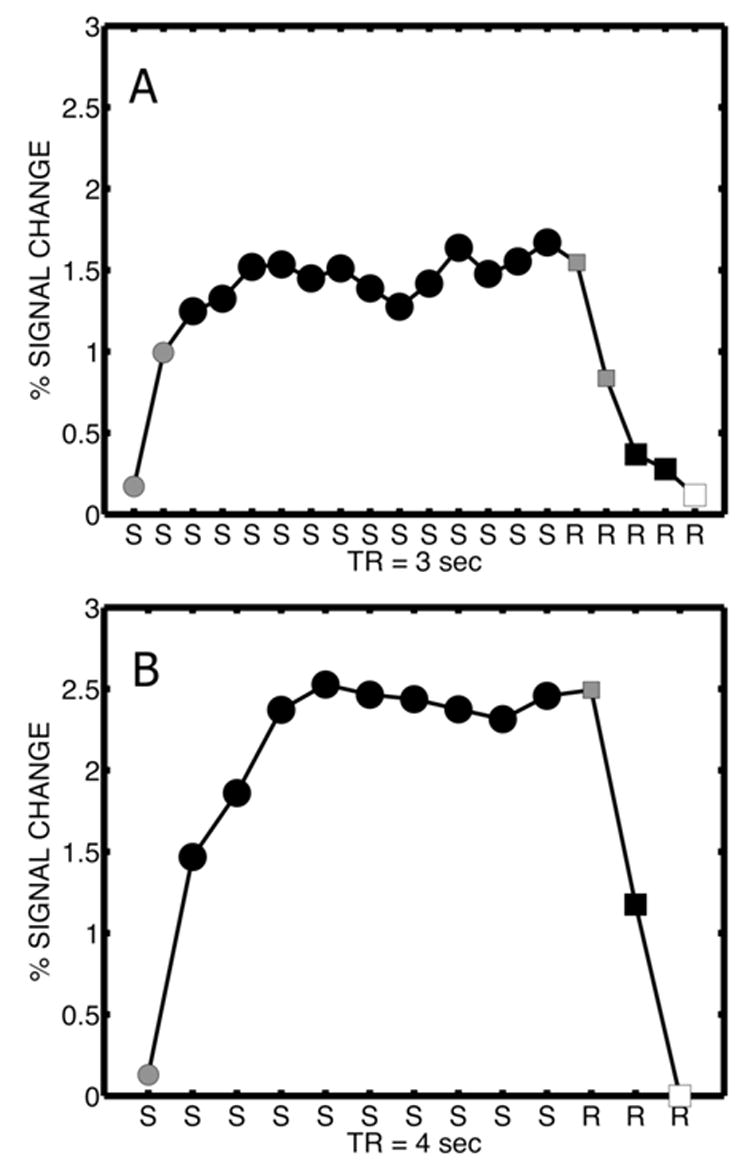
Response of an example occipital voxel is shown for protocol A (six subjects) and protocol B (two subjects). The two protocols involved different scanning rates and different numbers of stimulation frequencies as described in the text. The upper figure shows protocol A and the lower figure protocol B. Scans labeled S were stimulation scans and scans labeled R were resting scans. The voxel responses shown are shown for one block of stimulation and rest scans averaged
over all blocks (at different stimulation frequencies) and expressed for convenience as % signal change. The different symbols for the response label the use of scan for statistical analysis. The last resting scan, indicated by a white square, was used to detrend the signal, and to estimate % signal change. The solid black squares indicate scans used as “resting” control scans and solid circles indicate scans used as “stimulation” scans. Scans in grey symbols, at the transitions between stimulation and rest were discarded in the statistical analysis.
The statistical analysis was focused on the steady-state response. For both protocols, the first volume of each block of stimulation and the first resting volume immediately following the end of stimulation were discarded in order to exclude transient changes in the BOLD between conditions (indicated by gray circles). In protocol A, due to the use of faster scanning (TR=3 secs) the second scan of each block of stimulation and the second resting scan were also discarded as they likely also contained transients in the BOLD response. In protocol A (6 subjects), there were 26 volumes available for statistical analysis at each of 11 or 12 temporal frequencies (each frequency presented twice during the acquisition). In protocol B (2 subjects), there were 27 volumes at each of 19 temporal frequencies (each frequency presented thrice during the acquisition). One frequency (5 Hz) was repeated in the two separate acquisitions used in protocol B; they were treated as separate experimental conditions to check for consistency between the acquisitions.
Statistical analysis using tests described below was performed on individual subject data using MATLAB (Mathworks, Natick, MA) and the results were coregistered with the anatomical image for visualization using SPM2.
Identification of activated clusters
The first step in the data analysis was to identify clusters of voxels that were significantly modulated by the stimulus at one or more frequencies as compared to rest. One (Protocol B) or two (Protocol A) volumes from each block, indicated by a black square in Figure 1, were used as resting state for statistical analysis. The resting volumes used for the contrasts are drawn from volumes following all the stimulation frequencies to avoid stimulus-frequency specific effects. There were 33 or 36 resting volumes contrasted to 26 volumes for each stimulation frequency in protocol A; there were 30 resting volumes contrasted to 27 volumes for each stimulation frequency in protocol B.
The stimulation volumes at each reversal frequency were tested against the resting volumes using a Wilcoxon rank sum statistic (U), which is a test on the median value and can be approximated by a z score on the standard normal distribution for large sample sizes (Daniel, 1978). Each voxel was tested independently for each frequency and the highest value of |z| was the measure of activation. Clusters of at least 60 contiguous voxels where |z| > 1.96 (p < 0.05, two-tailed) were identified for further analysis. This procedure identified clusters of voxels that significantly deviated from the resting volumes during stimulation at one or more frequencies. No correction for multiple comparisons was used in this analysis, as the purpose was mainly exploratory to identify clusters for further analysis.
Statistical analysis of frequency dependence
A nonparametric one-way ANOVA (Kruskal-Wallis) was used to test for significant differences in the median value between stimulation at different frequencies for each voxel in an activated cluster. Each voxel was tested independently, and the resulting χ2 scores were compared to the threshold with degrees of freedom d equal to the number of frequencies minus 1. Significantly modulated voxels within each cluster were identified at the Bonferroni corrected significance level p < 0.05; the correction was calculated for each subject as the total number of voxels tested.
Correlation Analysis
We calculated the correlation coefficient (r) between every pair of voxels both within and across all clusters of voxels to quantify the similarity of responses. Correlation coefficients were calculated using only the stimulation volumes. Thus for protocol A, there were 26 volumes for each frequency and 11 or 12 frequencies; a total of 286 or 312 volumes were used to calculate the correlation coefficient. For protocol B, there were 27 volumes at each of 20 frequencies; a total of 540 volumes were used to calculate the correlation coefficient. The significance of each correlation coefficient was established at the p < 0.001 level using a t-test to test if the correlation coefficient is significantly different from zero (Bland 2000).
Display of fMRI results
For the purpose of averaging, anatomical localization, and display of the results, the subjects statistical maps were normalized to the MNI template and then de-normalized according to a single subject morphology (subject A1/B1) applying the respective inverse deformations using SPM2. The selected subject’s high resolution anatomical acquisition was treated with semiautomated tools for reconstruction of the brain’s cortical inflated surface (FreeSurfer, Fischl et al., 1999) and used as base for overlay of fMRI maps.
Results
Significant fMRI activation by the reversing checkerboard
Each subject showed strong activation of visual cortical areas in the occipital lobe as expected. In addition, each subject showed additional activations distributed in the basal medial frontal cortex. Figure 2 shows a map of the averaged |z|-scores across 6 subjects obtained when contrasting stimulation volumes to resting volumes indicating the two main clusters of significantly activated voxels (relative to resting blocks). The subjects exhibited larger fMRI responses during visual stimulation (as compared to rest) in a large number of voxels in the occipital cortex and a smaller number of voxels in the medial frontal lobes. A high degree of overlap of cluster location was also observed in the two subjects who repeated the experiment with the two protocols.
Figure 2.
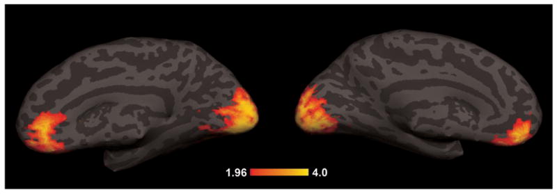
Subject-averaged functional activation map. The average of single subject statistical maps of the BOLD response is superimposed on an individual on a single subject (A1/B1) brain, first normalizing them to a common template then applying an inverse transformation to fit the selected subject anatomy. The hot scale represents z values with a threshold at p < 0.05 indicating a significant difference between stimulation volumes at any one frequency and the resting volumes using a Wilcoxon rank-sum test. In addition to the significance threshold, only clusters of at least 60 contiguous voxels with significant response were considered. Across all 6 subjects, the reversing checkerboard stimuli extensively activated both striate and extrastriate visual cortex and a part of the basal medial frontal cortex (BA 11, BA 10) according to Talairach coordinates.
Table 1 provides a summary of the results for all the subjects including the number of voxels in occipital and frontal clusters identified in each subject. In 5 of the 6 subjects the frontal voxels increased their response during stimulation (as compared to rest). In one subject (A3) the cluster in visual cortex increased response during stimulation similar to the other subject but the clustered voxels in frontal cortex, with similar location to the other subjects, significantly decreased their response relative to resting conditions. We included these voxels in the comparisons of responses between frequencies, since medial frontal cortex often shows high activity in the resting state (Gusnard et al., 2001) and our main interest was in the dependence of the responses on input frequency. None of the other subjects showed any clusters that significantly reduced their response to the stimulus.
Table 1.
Summary of results for occipital and frontal clusters.
| Subject | Occipital | Freq Mod (%) | Frontal | Freq Mod (%) |
|---|---|---|---|---|
| A1 | 393 | 51 (15) | 527 | 436 (83) |
| A2 | 262 | 22 (8) | 85 | 76 (89) |
| A3 | 569 | 11 (2) | 114* | 87 (75) |
| A4 | 367 | 49 (13) | 78 | 64 (82) |
| A5 | 441 | 32 (7) | 155 | 142 (92) |
| A6 | 424 | 108 (25) | 109 | 105 (96) |
| B1 | 416 | 67 (16) | 581 | 543 (93) |
| B2 | 277 | 34 (12) | 183 | 172 (94) |
Table 1. Summary of statistical results. The table presents the results of the cluster identification and frequency response function analysis described in the Methods section. The results are presented separately for Experiment A and B. For each subject two clusters of 60 or more voxels that significantly deviated (p < 0.05, two-tailed) from resting conditions were identified, one in occipital cortex, and one in frontal cortex. The number of voxels in each cluster and the number and % of these voxels in each cluster that show significant differences between frequencies are indicated.
Figure 3 shows a slice through the frontal lobes in each of our subjects with the z-score map overlaid on the anatomical image obtained after normalizing each subject’s data to a MNI template. We transformed the main coordinates of the clusters to the standard Talairach space (Talairach and Tournoux, 1988) and defined locations according to it. The frontal clusters are located within the Broadmann Areas BA 11 and BA 10, and, according to Talairach labeling, in the gyrus rectus and the medial orbito-frontal gyrus. One subject produced an unusually strong response centered on medial frontal but also extending to other areas in the prefrontal cortex in both protocols (A1/B1), always involving a larger number of voxels than in occipital cortex. Each of the other 5 subjects (A1/B1 and A3–A6) showed the largest cluster with the highest levels of response in the occipital cortex, and additional responses in frontal areas, always including a cluster in basal medial frontal cortex.
Figure 3.
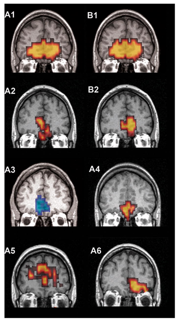
Individual subject activation maps in the frontal cortex. The significant mean BOLD response across frequencies compared to rest for each subject in a coronal slice. The individual brains and maps are normalized according to the MNI template and the selected slice is located at y = 46 mm. Hot and cold scales represent positive and negative z values, respectively. Only subject A3 shows a significant negative cluster. Both subjects 1 and 2 show the repeatability of results across protocols (A and B) while the subject A5 shows a more dorsal activation possibly due to a susceptibility artifact.
Dependence of the fMRI signal on reversal frequency
The voxels in each of the clusters in each subject were analyzed using a nonparametric one-way ANOVA (Kruskal-Wallis) to determine if the fMRI signal significantly varied between stimulus frequencies. Table 1 summarizes the % of significantly (Bonferroni-corrected p < 0.05) frequency-modulated voxels found in each of the clusters. Note that with this highly conservative criterion in each subject most of the activated voxels in the frontal cortex were also significantly frequency modulated. By contrast, few of the activated voxels in occipital cortex were significantly frequency modulated. Although the voxels in occipital cortex increased fMRI signal during stimulation versus rest, this response does not depend as strongly on stimulus frequency, in comparison to the frontal cortex response.
Figure 4 shows the median response of each voxel at each stimulation frequency, expressed as % signal change, for the two subjects A1/B1 and A2/B2 that repeated the experiment with the two protocols. The dependence of the response on stimulus frequency is presented as separate averages for the frontal (upper) and occipital voxels (lower) with the variability across voxels indicated by the error bars. The results for protocol B are presented on the left and protocol A are presented on the right. In both subjects, the responses of the frontal voxels are clearly frequency dependent, with the average over the frontal voxels (indicated by the filled square) reaching a maximum at a stimulation frequency equal to 4.5 Hz. This peak response was replicated in both protocols. By contrast, the average response of the occipital voxels appears to be relatively independent of frequency, as summarized by the statistical results in Table 1.
Figure 4.
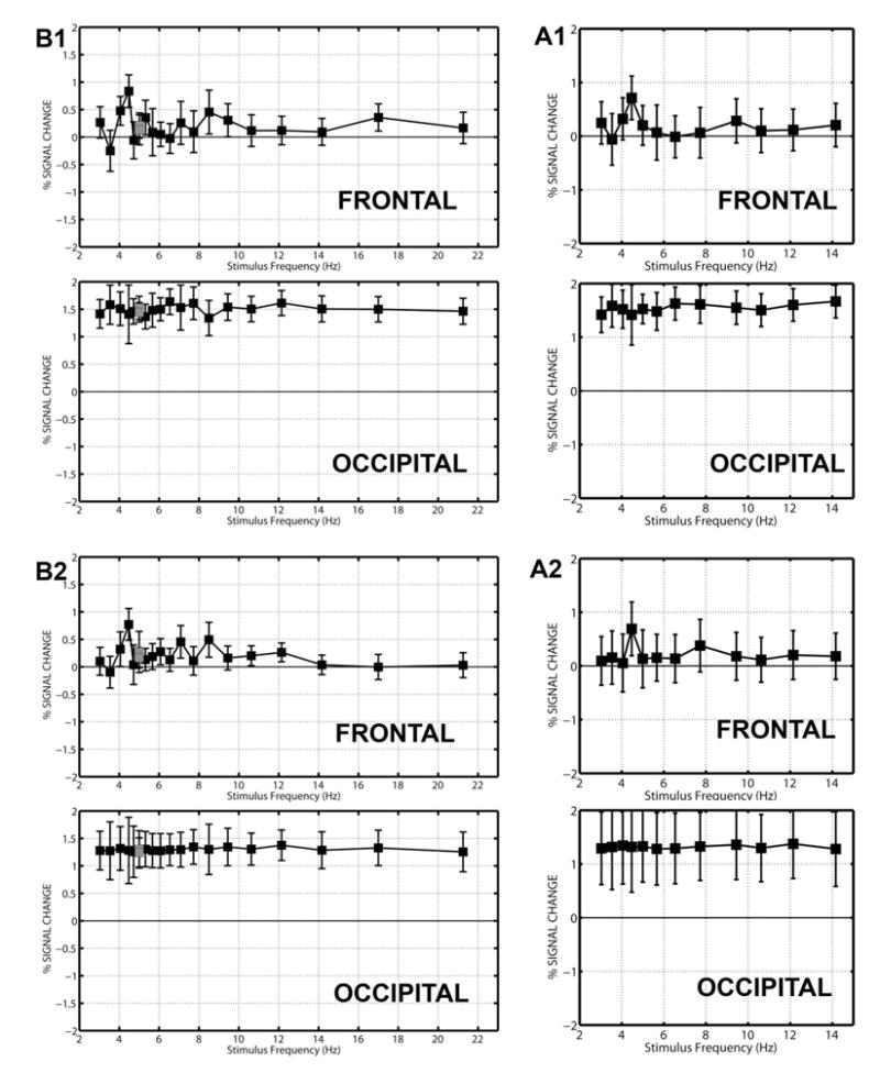
Average frequency response of frontal and occipital voxels in two subjects. These two subjects repeated the experiment with protocol A (A1 and A2) and B (B1 and B2). The response of each voxel was expressed as % signal change with reference to resting scans. At each frequency, the average response of the frontal (upper) and occipital (lower) voxels is indicated by the black square, and the error bars give the 95% confidence interval for the variability across voxels in the cluster. The number of frontal and occipital voxels for each subject in each protocol is given in Table 1.
Figure 5 shows the median response for each stimulation frequency for the other 4 subjects who participated in protocol A. In each subject the frontal voxels show an average response that depends on stimulus frequency, while the occipital voxels, on average, show a response that is relatively independent of stimulus frequency. The average response in three subjects (A3, A5, and A6) was highest at 5 Hz and increases in all the frontal voxels in comparison to other stimulation frequencies, as indicated by the error bars. In addition, subject A3 shows a strong decrease in response relative to rest at all frequencies. The other subject (A4) shows a peak at 3.5 Hz and a similar response at 4 Hz. Two subjects (A5 and A6) show secondary peaks at 4 Hz and 3 Hz respectively.
Figure 5.
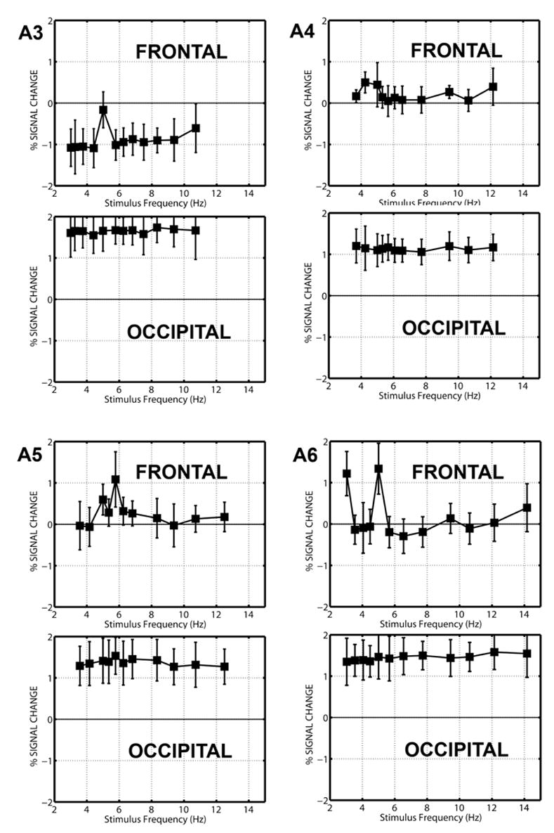
Average frequency response of frontal and occipital voxels in four subjects. The response of each voxel was expressed as % signal change with reference to resting scans. At each frequency, the average response of the frontal (upper) and occipital (lower) voxels is indicated by the black square, and the error bars give the 95% confidence interval for the variability across voxels in the cluster. The number of frontal and occipital voxels for each subject is given in Table 1.
Correlation analysis of an occipital-frontal network
Figure 6 shows the signal at three voxels, two occipital and one frontal from each volume in the low-frequency acquisition used in Protocol B, selected to best exemplify the pattern of correlation observed in this study. For each voxel, we first computed % signal change with reference to resting volumes and then removed the average response across all stimulation frequencies. For each frequency, the 27 values were sorted in ascending order of the responses at the medial frontal cluster and are indicated for each frequency by the black bars. The red and blue circles indicate the response for the two voxels in visual cortex on the corresponding volume.
Figure 6.
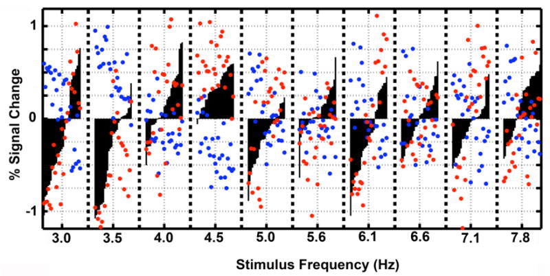
Frequency-dependent modulation of 3 individual voxels during one acquisition in one subject (B2). The response at three voxels, one in the medial frontal cortex (black bars), and two in visual cortex with different responses to input frequency (red circles and blue circles). For each voxel, the median response with respect to all stimulation frequencies has been subtracted from each point. The stimulation frequencies were presented in a pseudorandom order, and repeated 3 times, yielding 27 volumes per frequency. The 27 values for the medial frontal voxel (black bars) are presented for each frequency reordered in ascending order of the responses. The corresponding red and blue circles follow the same ordering and are the responses of two different voxels in the visual cluster.
Independent of the stimulation frequency, the response of one occipital voxel (red circles) generally increases when the response of the medial frontal voxel increases (black bars), while the response of the other occipital voxel (blue circles) decreases and vise versa. This is evident at the peak frequency of the medial frontal cluster (4.5 Hz), where frontal voxel and the occipital voxel shown in red show elevated responses on most volumes while the occipital voxel shown in blue decreases its response on most volumes. Even at other frequencies, e.g., 6.1 Hz, one occipital voxel (red circles) and the medial frontal voxels (black bars) show both higher or lower response in a consistent manner across the volumes at this frequency, with the opposite direction of response consistently exhibited by the other occipital voxel (blue circles). Using the data points shown in the figure, the correlation coefficient computed across all frequencies (270 volumes) between one visual voxel (red) and medial frontal voxel shown is positive (0.67) and between the other visual voxel (blue) and medial frontal voxel is negative (−0.68). Between the two voxels in visual cortex, the correlation coefficient is negative (−0.65).
Correlation coefficients were computed from all the stimulation volumes for each subject. Figure 7 shows a histogram of the correlation coefficients obtained from all pairs of voxels in the frontal and occipital cluster. The histogram was constructed for each subject and then averaged across subjects. The frontal voxels (F-F) are mostly positively correlated, while the occipital voxels (O-O) are both positively and negative correlated. The distribution of correlation coefficients between frontal and occipital voxels (F-O) is similarly bimodal. Figure 8 shows the correlation coefficients between all possible pairs of voxels in the frontal and occipital clusters. For two subjects the data from protocol B are shown, due to the larger number of volumes available; the results were very similar for protocol A. Each plot is divided into 4 unequal quadrants by black lines, and labeled along the axes. Along the diagonal the two quadrants correspond to frontal-frontal and occipital-occipital voxel pairs, while the two symmetric off-diagonal quadrants are correlation coefficients between one frontal and one occipital voxel.
Figure 7.
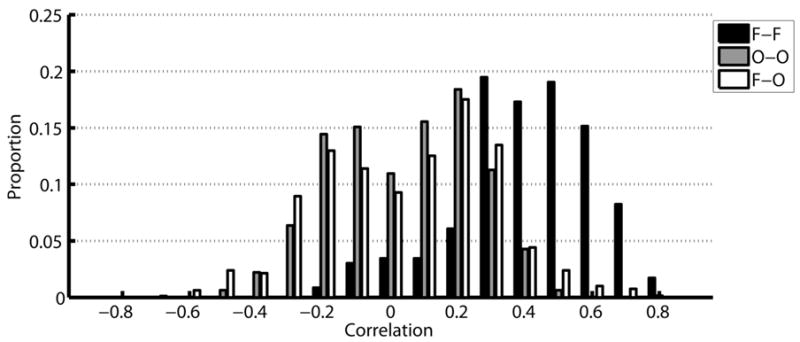
Subject-averaged histogram of the correlation between frontal and occipital clusters. For each subject, a histogram was calculated separately for correlation among voxels in the frontal cluster (F-F), among voxels in the occipital cluster (O-O) and between frontal and occipital voxels (F-O). The histograms were then averaged across subjects.
Figure 8.
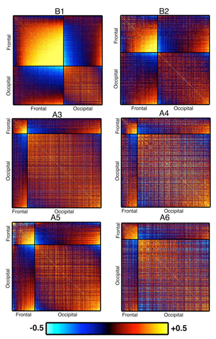
Correlation coefficients between voxels in each subject presented as a matrix. For 2 subjects (B1 and B2), the data from protocol B is shown, while for the other 4 subjects the data from protocol A are shown. The voxels are grouped into frontal and occipital voxels, which are labeled along the axis and separated by a black line. Thus each matrix plot is separated into 4 quadrants; the two quadrants along the diagonal correspond to correlations among the frontal and occipital voxels. The other two quadrants show identical correlation coefficients for pairs of voxels one from frontal cortex and the other from occipital cortex. The number of frontal and occipital voxels for each subject is given in Table 1. The hot scale indicates positive correlation coefficients and the cold scale negative correlation coefficients. A significance threshold (p < 0.001) was used to mask each correlation matrix.
In every subject, the voxels in the frontal cluster are almost entirely positively correlated to each other, with only a few voxel pairs exhibiting negative correlation, and were above 0.5 for many voxel pairs. Correlation coefficients among the occipital voxels were much lower, and were closely divided between positive and negative correlations. Some of these occipital voxels were positively correlated to the frontal voxels while others were negatively correlated to the frontal voxels. Strong positive and negative correlations between frontal and occipital voxels were found in each subject, suggesting the presence of two distinct functional networks among the occipital voxels.
To visualize the locations of these clusters, correlation coefficients were calculated between the signal at each frontal and occipital voxel, and the average signal of the frontal voxels. Figure 9 shows inflated maps for three subjects showing the spatial distribution of clusters in the occipital lobe that are positively and negatively correlated with the frontal activation. Subject B1 showed the highest frontal response, B2 showed more localized occipital responses while subject A3 best approximated the mean of all 6 subjects. While the location of the frontal cluster is very similar across subjects, the correlation of occipital voxels with the frontal voxels varied across subjects. In each subject, both primary and not primary visual areas appear to have both positively and negatively correlated clusters of voxels.
Figure 9.
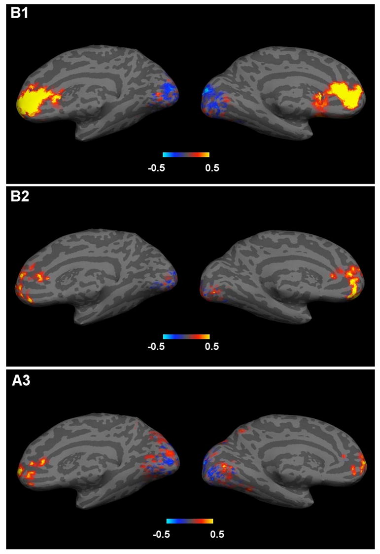
Maps of correlation coefficients between the average of the frontal clusters and all other voxels in the medial frontal and occipital clusters. The response of three representative subjects (B1, B2, A3), showing both common trend and variability, is presented on an inflated brain. Correlation maps were superposed on a single subject (A1/B1) brain, first normalizing them to a common template then applying an inverse transformation to fit the selected subject anatomy. The hot scale indicates positive correlation coefficients and the cold scale negative correlation coefficients.
Discussion
Steady-state paradigms in functional MRI
Steady-state methods have considerable potential for identifying functional networks in the human brain. They provide an excellent means to study fundamental neocortical dynamic processes since cortical inputs are (mostly) controlled. Although the details of the cortical dynamics elicited by visual stimulation are only partly known, we have no reason to believe that small changes in the temporal frequency at which the subject is stimulated, would change the inputs to the cortex. Thus, differences in measured brain activity due to changes in stimulation frequency can be mainly attributed to changes in the response of cortical populations. Theoretical models of cortical dynamics suggest that evidence of preferred input frequencies in different cortical areas reflects both properties of local circuits in each area and emergent properties of functional networks that involve cell assemblies in different cortical areas (Nunez, 2000; Habeck and Srinivasan, 2000; Nunez and Srinivasan, 2006).
In the present experiment the sinusoidal input is a reversing checkerboard and the measured output from the brain is the fMRI signal. In each of our subjects, we have found that a large number of voxels in occipital cortex and voxels in frontal cortex, including at least one cluster of voxels in medial frontal cortex exhibit significant activation by the visual input. The finding of fMRI activation in the medial frontal lobes by a visual input is consistent with anatomical data on the white-matter fiber systems oriented in the anterior-posterior direction of each hemisphere, some of which project from the occipital lobes to the basal medial frontal lobe (Kreig, 1963; Kreig, 1973). In the medial frontal lobe, most, and often all, of the activated voxels show highly significant modulation of the response by the temporal frequency of the visual input. A peak frequency in the range of 3.5–5 Hz was found in medial frontal cortex in all the subjects. The location of the frontal cluster and the peak frequency was replicated in the two subjects who participated in the two protocols on different days. Thus, fMRI signals can be used to detect frequency-specific cortical responses.
Comparisons with SSVEP recordings using EEG and MEG
This frequency-specificity of the frontal response is qualitatively consistent with previous EEG and MEG studies that show that the steady-state responses to flicker at sensors or electrodes over frontal and prefrontal areas exhibit strongest responses at flicker frequencies in the range of 8–12 Hz (Narici et al., 1998; Nunez, 1995; Srinivasan et al., 1999; Srinivasan, 2004). When using a reversing contrast stimulus, as in the present fMRI experiment, the largest response in the EEG or MEG occurs at the second harmonic (double the stimulus frequency); responses are only found at the even harmonics, but no response is observed at the fundamental or odd harmonics (Regan, 1989). The highest SSVEP magnitude was found with stimulus frequencies ranging from 4–5 Hz which elicits a second harmonic response at 8–10 Hz. In the present fMRI study, we measured the effect of the reversing checkerboard on fMRI signals at different stimulus frequencies in comparison to rest. Because fMRI is measured on a slower time scale the harmonic structure of the neural response is not observable. Thus, fMRI responses to flicker reflect not only the steady-state responses at the harmonic frequencies but potentially also including asynchronous responses to the stimulus that are not observed with EEG/MEG (Nunez and Silberstein, 2000).
Over a broad range of stimulus frequencies (3–21 Hz), we found that most voxels in occipital cortex responded to the stimulus; but in all our subjects most voxel responses did not vary significantly with stimulus frequency. These findings are quite different from EEG/MEG studies that have found robust evidence of resonance frequencies at electrodes over occipital cortex (Regan, 1989; Srinivasan, 2004). Over a comparable range of frequencies, EEG responses to flicker or checkerboard reversal vary by more than one order of magnitude at occipital electrodes (Herrmann, 2001; Regan, 1989; Srinivasan, 2004; Ding et al., 2006; Srinivasan et al., 2006). This difference may be the results of the difference in spatial and temporal resolution between EEG/MEG and fMRI. EEG/MEG signals are space averages over relatively large area of the cortical surface (> 20 cm2) with high temporal resolution (Nunez, 1981; Srinivasan et al., 1996; Srinivasan et al., 1998; Nunez and Srinivasan, 2006). Thus EEG and MEG are sensitive to the phase difference between neural populations oscillating at the stimulus frequency distributed over the cortical surface, and relatively strong sources that are closely positioned may in fact cancel at the EEG electrode (or MEG sensor) if they are 180 degrees out of phase. Even if the phases of all sources are identical within a cortical region, cancellation can take place only due to geometrical factors, for instance due to sources positioned in opposite walls of a sulcus (Nunez, 1981; Nunez and Srinivasan, 2006). By contrast, the fMRI response has low temporal resolution and is insensitive to the phases of the activity in neural populations. It is well known from EEG studies that the phase of the steady-state response depends strongly on the input frequency, partly reflecting the delay between retina and primary visual cortex, and delays in transmission between areas of the visual system (Schmolesky et al., 1998). In any linear system constant delays produce increasing phase as temporal frequency increases (Bendat and Piersol, 2000), while in nonlinear systems more complex relationships between delays and the phase of the response can be anticipated. In either case, periodic input at any frequency, responses of populations in the visual system can reasonably be expected to be distributed in phase, in a manner than depends on the stimulus frequency (Nunez, 1995). We can conjecture that the striking differences between EEG/MEG and fMRI in occipital cortex are due to the phase patterns among populations in visual cortex elicited by different stimulus frequencies influencing only the EEG/MEG signals.
Frequency-dependent Occipital-Frontal networks
The results of the present fMRI experiment support the hypothesis that functional connectivity of the human brain is frequency-dependent. A large body of electrophysiological studies also support this general hypothesis (von Stein and Sarnthein, 2000; Engel et al., 2001; Knyazeva et al., 2006), although the relative importance of specific frequencies to specific cognitive processes remains controversial (Habeck and Srinivasan, 2000). The use of steady-state methods in fMRI studies has the potential to provide a mapping of functional connectivity that incorporates, in an indirect manner, dynamical properties of the functional connection.
In this study we found a cluster of voxels in medial frontal cortex that responds at a preferred frequency in the 3.5–5 Hz range and that some voxels in occipital cortex are positively correlated to the medial frontal voxels at all frequencies. This correlation between responses at very distant voxels, suggests the presence of a functional network involving part of the occipital cortex and medial frontal lobe, but probably also involving other areas of the brain (but below the threshold for MR activation). While we have not directly investigated the functions of this network in this simple visual stimulation fMRI experiment, our EEG and MEG studies have shown that the responses to flicker recorded at midline frontal EEG or MEG channels increase when attention is directed to the flicker (Ding et al., 2006) and exhibit increased phase-locking when the flicker is consciously perceived during binocular rivalry (Srinivasan and Petrovic, 2006).
We observe negative correlation between occipital voxels consistent with the notion that voxels in occipital cortex can be modulated in opposite directions by stimulus features such as flicker frequency. This finding is similar to reports of suppression of the BOLD signal by stimulus presentation. It has been demonstrated in visual cortex that a visual stimulus can elicit both positive and negative BOLD responses, suggesting that both increases and decreases of neural activity can be genuinely elicited by a visual stimulus (Saad et al., 2001; Shmuel et al., 2002). However, in this study, we have not observed a robust negative response, only a negative correlation between the responses.
Methodological considerations
The designs of steady-state experiments are potentially useful for future investigation of EEG-fMRI relationships, and co-registration of EEG sources with fMRI. In EEG or MEG studies using steady-state paradigms the typical duration of stimulation is chosen as at least 10 secs, corresponding to a frequency resolution of 0.1 Hz or less to obtain very high signal-to-noise ratios (Srinivasan, 2004). Thus, the temporal scales of the steady-state EEG/MEG and fMRI responses can be easily matched. The steady-state resonance exhibits spatial properties that strongly depend on the driving frequency, suggestive of resonant modes in physical systems (Nunez, 1995; Nunez, 2000; Nunez and Srinivasan, 2006; Srinivasan et al., 2006). This property is particularly useful for investigating EEG-fMRI relationships since we can change in both the EEG or MEG amplitude and distribution and fMRI responses with a small change in the driving frequency (i.e., with nearly identical spatial patterns of input to the cortex) to examine if the differences between frequencies are similar in EEG and fMRI.
Conclusions
The results of our study demonstrate robust frequency dependence of the fMRI in medial frontal lobe in 6 human subjects. This preliminary result indicates that visually-driven functional networks of the brain may have distinct spatial distributions across different cortical areas with characteristic frequencies that can be assessed using fMRI. In this study we have used he simplest stimulus, a reversing checkerboard, and elicited a response in the frontal lobes. With more complex stimuli and cognitive tasks, we anticipate engaging other cortical areas, as suggested by the distributed, task-modulated, frequency-dependent responses evident in EEG and MEG studies. This essential idea of frequency-dependent functional connectivity is consistently found in many electrophysiological studies in animals and humans with electrodes at different locations and at different spatial scales (Singer 1999a,b; von Stein and Sarnthein, 1998; von Stein et al. 2000; Srinivasan et al., 1999; Srinivasan, 2004; Nunez and Srinivasan, 2006; Srinivasan et al., 2006; Knyazeva et al., 2006).
Acknowledgments
This research was supported by a Visiting Fellowship from the Novartis Consumer Health Foundation to RS, a grant from the NIH R01-MH68004 and by Swiss National Science Foundation grant #31-63894.00.
References
- Bendat JS, Piersol A. Random Data: Analysis and Measurement Procedures. 3. Wiley; NY: 2000. [Google Scholar]
- Bland M. An Introduction to Medical Statistics. 3. Oxford University Press; New York: 2000. [Google Scholar]
- Brainard DH. The Psychophysics Toolbox. Spat Vis. 1997;10:433–6. [PubMed] [Google Scholar]
- Chen Y, Seth AK, Gally JA, Edelman GM. The power of human brain magnetoencephalographic signals can be modulated up or down by changes in an attentive visual task. Proc Natl Acad Sci U S A. 2003;100:3501–6. doi: 10.1073/pnas.0337630100. [DOI] [PMC free article] [PubMed] [Google Scholar]
- Daniel W. Applied Nonparametric Statistics. Houghton Mifflin; 1978. [Google Scholar]
- Ding J, Sperling G, Srinivasan R. Attentional modulation of SSVEP power depends on the network tagged by the flicker frequency. Cereb Cortex. 2006;16:1016–29. doi: 10.1093/cercor/bhj044. [DOI] [PMC free article] [PubMed] [Google Scholar]
- Engel AK, Fries P, Singer W. Dynamic predictions: oscillations and synchrony in top-down processing. Nat Rev Neurosci. 2001;2:704–16. doi: 10.1038/35094565. [DOI] [PubMed] [Google Scholar]
- Fischl B, Sereno MI, Dale AM. Cortical surface-based analysis II: inflation, flattening, and a surface-based coordinate system. NeuroImage. 1999;9 :179–194. doi: 10.1006/nimg.1998.0396. [DOI] [PubMed] [Google Scholar]
- Fox PT, Raichle ME. Stimulus rate dependence of regional cerebral blood flow in human striate cortex, demonstrated by positron emission tomography. J Neurophysiology. 1984;51:1109–1120. doi: 10.1152/jn.1984.51.5.1109. [DOI] [PubMed] [Google Scholar]
- Gusnard DA, Akbudak E, Shulman GL, Raichle ME. Medial prefrontal cortex and self-referential mental activity: relation to a default mode of brain function. PNAS USA. 2001;98:4259–4264. doi: 10.1073/pnas.071043098. [DOI] [PMC free article] [PubMed] [Google Scholar]
- Habeck CG, Srinivasan R. Natural solutions to the problem of functional integration. Behavioral and Brain Sciences. 2000;23:402–403. [Google Scholar]
- Hagenbeek RE, Rombouts SARB, van Dijk BW, Barkhof F. Determination of Individual Stimulus-Response Curves in the Visual Cortex. Human Brain Mapping. 2002;17:244–250. doi: 10.1002/hbm.10067. [DOI] [PMC free article] [PubMed] [Google Scholar]
- Herrmann CS. EEG responses to 1–100 Hz flicker: resonance phenomena in visual cortex and their potential correlation to cognitive phenomena. Exp Brain Res 2001. 2001;137:346–53. doi: 10.1007/s002210100682. [DOI] [PubMed] [Google Scholar]
- Knyazeva MG, Fornari E, Meuli R, Maeder P. Interhemispheric integration at different spatial scales: the evidence from EEG coherence and FMRI. J Neurophysiol. 2006;96:259–75. doi: 10.1152/jn.00687.2005. [DOI] [PubMed] [Google Scholar]
- Kreig WJS. Architectonics of Human Cerebral fiber Systems. Brain Books; Evanston IL: 1973. [Google Scholar]
- Kreig WJS. Connections of the Cerebral Cortex. Brain Books; Evanston IL: 1963. [Google Scholar]
- Kwong KK, Belliveau JW, Chesler DA, Goldberg IE, Weisskoff RM, Poncelet BP, Kennedy DN, Hoppel BE, Cohen MS, Turner R, Cheng HM, Brady TJ, Rosen BR. Dynamic magnetic resonance imaging during primary sensory stimulation. PNAS USA. 1992;89:5675–5679. doi: 10.1073/pnas.89.12.5675. [DOI] [PMC free article] [PubMed] [Google Scholar]
- Mentis MJ, Alexander GE, Grady CL, Horowitz B, Krasuski J, Pietrini P, Strassburger T, Hampel H, Schapiro MB, Rapoport SI. Frequency variation of a pattern-flash visual stimulus during PET differentially activates brain from striate through frontal cortex. Neuroimage. 1997;5:116–128. doi: 10.1006/nimg.1997.0256. [DOI] [PubMed] [Google Scholar]
- Muller MM, Teder W, Hillyard SA. Magnetoencephalographic recording of steady-state visual evoked cortical activity. Brain Topogr. 1997;9:163–8. doi: 10.1007/BF01190385. [DOI] [PubMed] [Google Scholar]
- Nakayama K, Mackeben M. Steady-state visual evoked potentials in the alert primate. Vision Research. 1982;22:1261–1271. doi: 10.1016/0042-6989(82)90138-9. [DOI] [PubMed] [Google Scholar]
- Narici L, Portin K, Salmelin R, Hari R. Responsiveness of Human Cortical activity to rhythmical stimulation: A three-modality, whole cortex neuromagnetic investigation. 1998;7:209–223. doi: 10.1006/nimg.1998.0323. [DOI] [PubMed] [Google Scholar]
- Nunez PL. Electric Fields of the Brain: The Neurophysics of EEG. Oxford; NY: 1981. [Google Scholar]
- Nunez PL. Neocortical dynamics and human EEG rhythms. Oxford; NY: 1995. [Google Scholar]
- Nunez PL. Towards a quantitative description of neocortical dynamic function and EEG. Behavioral and Brain Sciences. 2000;23:371–437. doi: 10.1017/s0140525x00003253. [DOI] [PubMed] [Google Scholar]
- Nunez PL, Silberstein RB. On the relationship of synaptic activity to macroscopic measurements: Does co-registration of EEG with fMRI make sense? Brain Topography. 2000;13:79–96. doi: 10.1023/a:1026683200895. [DOI] [PubMed] [Google Scholar]
- Nunez PL, Srinivasan R. Electric Fields of the Brain: The Neurophysics of EEG. 2. Oxford University Press; New York: 2006. [Google Scholar]
- Rager G, Singer W. The response of the cat visual cortex to flicker stimuli of variable frequency. Eur J Neurosci. 1998;10:1856–1877. doi: 10.1046/j.1460-9568.1998.00197.x. [DOI] [PubMed] [Google Scholar]
- Regan D. Steady-state evoked potentials. J Opt Soc Am. 1977;67:1475–89. doi: 10.1364/josa.67.001475. [DOI] [PubMed] [Google Scholar]
- Regan D. Human brain electrophysiology. New York; Elsevier: 1989. [Google Scholar]
- Saad ZS, Ropelia KM, Cox RW, DeYoe EA. Analysis and use of fMRI response delays. Human Brain Mappin. 2001;13:74–93. doi: 10.1002/hbm.1026. [DOI] [PMC free article] [PubMed] [Google Scholar]
- Schmolesky MT, Wang Y, Hanes DP, Thompson KG, Leutgeb S, Schall JD, Leventhal AG. Signal timing across the macaque visual system. Journal of Neurophysiology. 1998;79:3272–3278. doi: 10.1152/jn.1998.79.6.3272. [DOI] [PubMed] [Google Scholar]
- Shmuel A, Yacoub E, Pfeuffer J, Van der Moortele PF, Adriany G, Hu X, Ugurbil K. Sustained negative BOLD, Blood Flow, and oxygen consumption response and its coupling to positive response in the human brain. Neuron. 2002;36:1195–1210. doi: 10.1016/s0896-6273(02)01061-9. [DOI] [PubMed] [Google Scholar]
- Silberstein RB, Nunez PL, Pipingas A, Harris P, Danieli F. Steady state visually evoked potential (SSVEP) topography in a graded working memory task. International Journal of Psychophysiology. 2001;42:219–32. doi: 10.1016/s0167-8760(01)00167-2. [DOI] [PubMed] [Google Scholar]
- Silberstein RB. Steady state visually evoked potentials, brain resonances and cognitive processes. In: Nunez PL, editor. Neocortical Dynamics and Human EEG Rhythms. Oxford University Press; New York: 1995. [Google Scholar]
- Silberstein RB, Danieli F, Nunez PL. Fronto-parietal evoked potential synchronization is increased during mental rotation. Neuroreport. 2003;14:67–71. doi: 10.1097/00001756-200301200-00013. [DOI] [PubMed] [Google Scholar]
- Silberstein RB, Song J, Nunez PL, Park W. Dynamic sculpting of brain functional connectivity is correlated with performance. Brain Topogr. 2004;16:249–254. doi: 10.1023/b:brat.0000032860.04812.b1. [DOI] [PubMed] [Google Scholar]
- Singer W. Striving for coherence. Nature. 1999a;397:391–3. doi: 10.1038/17021. [DOI] [PubMed] [Google Scholar]
- Singer W. Neural synchrony, a versatile code for the definition of relations? Neuron. 1999b;24:49–65. doi: 10.1016/s0896-6273(00)80821-1. [DOI] [PubMed] [Google Scholar]
- Singh M, Kim S, Kim TS. Correlation between BOLD-fMRI and EEG signal changes in response to visual stimulus frequency in humans. Magnetic resonance in medicine. 2003;49:108–114. doi: 10.1002/mrm.10335. [DOI] [PubMed] [Google Scholar]
- Srinivasan R. Internal and external neural synchronization during conscious perception. International Journal of Bifurcation and Chaos. 2004;19:1–18. doi: 10.1142/S0218127404009399. [DOI] [PMC free article] [PubMed] [Google Scholar]
- Srinivasan R, Bibi FA, Nunez PL. Steady-state visual evoked potentials: distributed local sources and wave-like dynamics are sensitive to flicker frequency. Brain Topogr. 2006;18:167–87. doi: 10.1007/s10548-006-0267-4. [DOI] [PMC free article] [PubMed] [Google Scholar]
- Srinivasan R, Nunez PL, Silberstein RB. Spatial filtering and neocortical dynamics: estimates of EEG coherence. IEEE Trans Biomed Eng. 1998;45:814–26. doi: 10.1109/10.686789. [DOI] [PubMed] [Google Scholar]
- Srinivasan R, Nunez PL, Tucker DM, Silberstein RB, Cadusch PJ. Spatial sampling and filtering of EEG with spline laplacians to estimate cortical potentials. Brain Topogr. 1996;8:355–66. doi: 10.1007/BF01186911. [DOI] [PubMed] [Google Scholar]
- Srinivasan R, Petrovic S. MEG phase follows conscious perception during binocular rivalry induced by visual stream segregation. Cereb Cortex. 2006;16:597–608. doi: 10.1093/cercor/bhj016. [DOI] [PMC free article] [PubMed] [Google Scholar]
- Srinivasan R, Russell DP, Edelman GM, Tononi G. Increased synchronization of neuromagnetic responses during conscious perception. Journal of Neuroscience. 1999;19:5435–48. doi: 10.1523/JNEUROSCI.19-13-05435.1999. [DOI] [PMC free article] [PubMed] [Google Scholar]
- Talairach J, Tournoux P. Co-planar Stereotaxic Atlas of the Human Brain. Thieme Medical Publishers; New York: 1988. [Google Scholar]
- Thomas CG, Menon RS. Amplitude response and stimulus presentation frequency response of human primary visual cortex using BOLD EPI at 4T. Magnetic Resonance in Medicine. 1998;40:203–209. doi: 10.1002/mrm.1910400206. [DOI] [PubMed] [Google Scholar]
- Tononi G, Srinivasan R, Russell DP, Edelman GM. Investigating neural correlates of conscious perception by frequency-tagged neuromagnetic responses. Proc Natl Acad Sci U S A 1998. 1998;95:3198–203. doi: 10.1073/pnas.95.6.3198. [DOI] [PMC free article] [PubMed] [Google Scholar]
- Tyler CW, Apkarian P, Nakayama K. Multiple spatial frequency tuning of electrical responses from the human visual cortex. Experimental Brain Research. 1978;33:535–550. doi: 10.1007/BF00235573. [DOI] [PubMed] [Google Scholar]
- von Stein A, Chiang C, Konig P. Top-down processing mediated by interareal synchronization. Proc Natl Acad Sci U S A. 2000;97:14748–53. doi: 10.1073/pnas.97.26.14748. [DOI] [PMC free article] [PubMed] [Google Scholar]
- von Stein A, Sarnthein J. Different frequencies for different scales of cortical integration: from local gamma to long range alpha/theta synchronization. International Journal of Psychophysiology. 2000;38:301–313. doi: 10.1016/s0167-8760(00)00172-0. [DOI] [PubMed] [Google Scholar]