A simplified approach to quasi-linear viscoelastic modeling

Abstract

The fitting of quasi-linear viscoelastic (QLV) constitutive models to material data often involves somewhat cumbersome numerical convolution. A new approach to treating quasi-linearity in one dimension is described and applied to characterize the behavior of reconstituted collagen. This approach is based on a new principle for including nonlinearity and requires considerably less computation than other comparable models for both model calibration and response prediction, especially for smoothly applied stretching. Additionally, the approach allows relaxation to adapt with the strain history.

The modeling approach is demonstrated through tests on pure reconstituted collagen. Sequences of “ramp-and-hold” stretching tests were applied to rectangular collagen specimens. The relaxation force data from the “hold” was used to calibrate a new “adaptive QLV model” and several models from literature, and the force data from the “ramp” was used to check the accuracy of model predictions. Additionally, the ability of the models to predict the force response on a reloading of the specimen was assessed.

The “adaptive QLV model” based on this new approach predicts collagen behavior comparably to or better than existing models, with much less computation.

1. Introduction

Nonlinear viscoelastic behavior can be modeled within a very general framework (Coleman and Noll, 1961). Calibrating a general framework to specific materials can be challenging, especially for highly variable biological tissues. For these materials, Fung’s quasi-linear viscoelastic (QLV) model (Fung, 1993) is attractive: it identifies a class of quasi-linearity that is appropriate for many tissues, thereby simplifying model calibration.

Fung’s QLV model has two limitations. First, it cannot always achieve the desired accuracy, due to its limitation that the stress response resulting from any level of instantaneous straining must be proportional to a single “reduced” relaxation function. For example, Provenzano et al. (2001) observed that stress relaxation curves are not proportional to a single reduced relaxation function in rat medial collateral ligaments, and we observed this in our previous work in pure, reconstituted collagen (Pryse et al., 2003). This limitation can be overcome by increasing the number of degrees of freedom, as in the “generalized Fung model” we proposed (Pryse et al. 2003).

However, increasing the number of degrees of freedom compounds the second limitation of Fung’s QLV model, which is the need for complicated numerical procedures for calibration. The model parameters to be calibrated in the Fung QLV model and our generalization are convolved functions, except when data is available for stresses resulting from a perfect instantaneous step stretch. We have found that this limits not only the ease of calibration, but also model accuracy in some cases, motivating us to look for an accurate and easier to calibrate alternative.

We present an alternative approach for including nonlinearity in linear viscoelastic equations, in which the nonlinearity is partitioned so as to simplify model calibration, and we show the ability of the resulting “adaptive QLV model” to predict the nonlinear viscoelastic behavior of reconstituted collagen gels. The nonlinear “mechanical elements” of the adaptive QLV model differ from those of the Fung QLV model, but the adaptive approach retains the Fung QLV model’s flexibility. Like Fung’s QLV model, ours is phenomenological: when calibrated to the results of a few tests, it predicts subsequent viscoelastic behavior (Hsu et al., 1994; Johnson et al., 1996; Ozerdem and Tozeren, 1995; Pioletti et al., 1998; Provenzano et al., 2002; Pryse et al., 2003). This contrasts with models using the structure of collagen (Alberts et al., 1994) to predict behavior from properties of individual collagen molecules (Misof et al., 1997; Parry, 1988) or fibers (Christiansen et al., 2000; Decraemer et al., 1980; Lanir, 1983; Pins et al., 1997; Sacks, 2003; Silver et al., 2000; Thomopoulos et al., 2006; Thornton et al., 2001; Wagenseil et al., 2003).

After reviewing Fung’s QLV model and providing a generalized definition of quasi-linearity, we present the adaptive model and compare its predictive ability to that of other models. Testing involves calibration of models using “hold” data from “ramp-and-hold” tests, then prediction of both the “ramp” portion of these same tests and of the mechanical response in a subsequent reloading of the same specimens. The adaptive QLV model has advantages in ease of calibration, and is comparable to or better than an existing generalization of Fung’s QLV model in its predictive capability.

2. Background

We review for comparison Fung’s QLV model and define quasi-linearity. The “generalized Fung model” we also consider is described elsewhere (Pryse et al., 2003).

2.1 Fung’s QLV Model

In Fung’s QLV model, stress is calculated through a linear convolution integral:

$$\begin{array}{l}\sigma (t)=\underset{-\infty }{\overset{t}{\int }}g(t-\xi )\frac{d{\sigma }^{(e)}(\epsilon (\xi ))}{d\xi }d\xi \\ =\underset{-\infty }{\overset{t}{\int }}g(t-\xi )\frac{d{\sigma }^{(e)}(\epsilon )}{d\epsilon }\frac{d\epsilon (\xi )}{d\epsilon }d\xi ,\end{array}$$ (1)

where σ is uniaxial stress, ε is the corresponding strain, g(t) is the “reduced” relaxation function, normalized by its initial value (g(0)=1), and σ^(e)(ε) is a function of strain called the “elastic stress.” Nonlinearity is included within the elastic tangent stiffness term, dσ^(e)(ε)/dε, and g(t) may be chosen to model different materials (Abramowitch and Woo, 2003). A common choice of g(t) is $g(t)=a_o+{\displaystyle \underset{i}{\Sigma }}{a}_i{e}^{-t/{\tau }_i}$, where each time constant is associated with a series combination of spring and dashpot with normalized spring constant a_i, and a_o is associated with a spring. Fung (1993) proposed a continuous spectrum of time constants S(τ):

$$g(t)=\frac{1+{\int }_0^{\infty }S(\xi )e^{-t/\xi }d\xi }{1+{\int }_0^{\infty }S(\xi )d\xi }.$$

Fung applied S(τ) = c/τ, as done independently by Neubert (1963) to describe rubber viscoelasticity.

2.2 Quasi-Linearity

Fung’s QLV model is quasi-linear in the sense that the dependence of response on loading history can be obtained from a linear convolution integral, which preserves the benefits of linearity for calibrating the model, simplifies model predictions, and permits meaningful analysis in Fourier and Laplace space. Nonlinearity enters the linear viscoelastic constitutive law by replacing strain with a nonlinear function of strain, and the resultant model is linear with respect to a pure function of strain instead of strain itself.

We expand the term quasi-linear viscoelastic to encompass nonlinear viscoelastic constitutive laws in which loading history dependence can be modeled by a linear convolution integral or a summation of linear convolution integrals. A feature of such QLV models is that the stress and strain (force and displacement) are related by an intermediate variable that separates the nonlinearity from the viscoelasticity. In Fung’s QLV model, the “elastic stress” is the intermediate variable that allows use of a linear convolution integral to derive stress.

3. Adaptive QLV Model

3.1 Mathematical Framework

We related stress and strain through an intermediate variable, a “viscoelastic strain,” V^(ε)(t), in a linear convolution integral:

$$\begin{array}{l}\sigma (t)=k(\epsilon (t))V^{(\epsilon )}(t)\\ V^{(\epsilon )}(t)=\underset{-\infty }{\overset{t}{\int }}g(t-\xi )\frac{d\epsilon (\xi )}{d\xi }d\xi ,\end{array}$$ (2)

where k(ε) is a pure nonlinear function of strain, and, following Fung, g(t) is a “reduced” relaxation function that can be expressed as a summation of exponentials with different time constants. V^(ε)(t) represents the dependence of the model on loading history. The nonlinearity of the model lies in k(ε), which converts the viscoelastic strain to stress by a simple multiplication. Similar to the Fung QLV model, Equation (2) generates proportional stress relaxations for different amplitudes of instantaneous strain. To overcome this proportionality restriction we added degrees of freedom to the model by allowing different nonlinear behavior for different time constants:

$$\begin{array}{c}\sigma (t)={\sigma }_o(\epsilon (t))+\underset{i}{\Sigma }{k}_i(\epsilon (t))V_i^{(\epsilon )}(t)\\ V_i^{(\epsilon )}(t)=\underset{-\infty }{\overset{t}{\int }}{g}_i(t-\xi )\frac{d\epsilon (\xi )}{d\xi }d\xi \end{array}\hspace{0.17em}\hspace{0.17em}\hspace{0.17em}i=1,2,\dots$$ (3)

where σ₀(ε) is a pure function of strain representing the fully relaxed elastic response. Each (t) could be any relaxation function such that g(0)=1 and g(∞)=0. We chose g_i(t) = e^−t/^τ_i to represent the model in terms of parallel Maxwell elements (Figure 1), although such elements need not exist physically.

Figure 1.

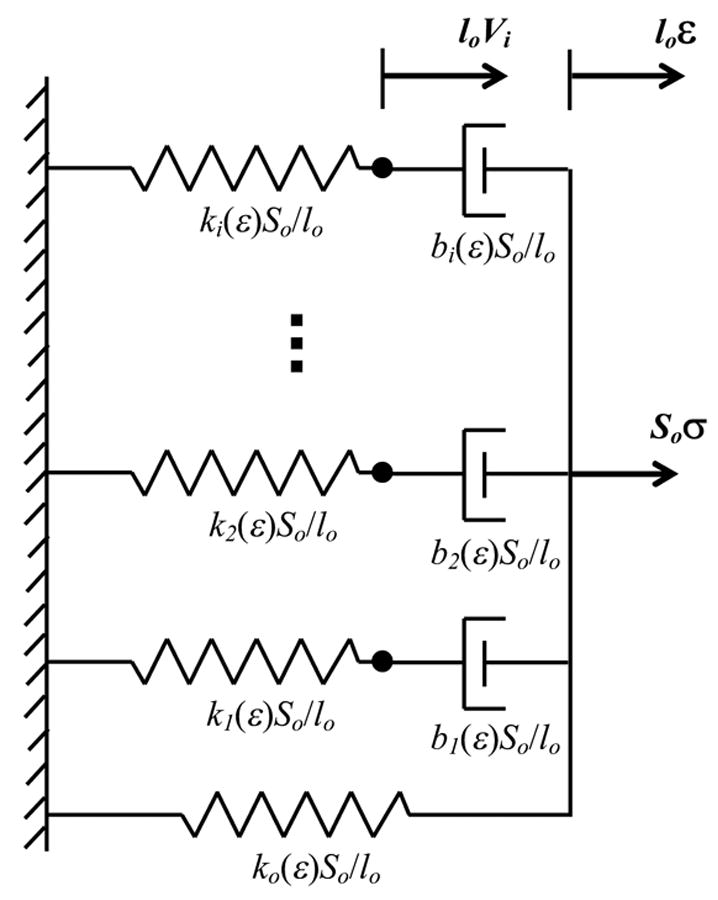
1-D “spring and dashpot” representation of the adaptive QLV model, a parallel combination of nonlinear springs and dashpots where the spring stiffnesses and dashpot coefficients are functions of overall strain and not their individual strain. S_o is the initial cross section of specimen, l_o is the initial length of specimen, l_oV_i is the displacement of the hypothetical spring and ε and σ are uniaxial, linearized strain and stress, respectively.

For each hypothetical Maxwell element,

$$\{\begin{array}{l}{\dot{V}}_i+\frac{V_i}{{\tau }_i(\epsilon )}=\dot{\epsilon }\hfill \\ {\sigma }_i=k_i(\epsilon (t))V_i(t)\hfill \end{array},i=1,2,\dots$$ (4)

where:

$${\tau }_i(\epsilon )=\frac{b_i(\epsilon )}{k_i(\epsilon )},$$

and for the spring representing the fully relaxed elastic response:

$${\sigma }_o={\sigma }_o(\epsilon ).$$

This nonlinear viscoelastic model becomes quasi-linear by assigning each pair of spring stiffness and dashpot coefficients to be proportional to the same nonlinear function of strain:

$$\{\begin{array}{l}{k}_i(\epsilon )={\eta }_i{\psi }_i(\epsilon )\hfill \\ b_i(\epsilon )={\beta }_i{\psi }_i(\epsilon )\hfill \end{array},$$

where ψ_i(ε) are arbitrary nonzero functions, making each time constant τ_i independent of strain:

$${\tau }_i(\epsilon )=\frac{b_i(\epsilon )}{k_i(\epsilon )}=\frac{{\beta }_i}{{\eta }_i}={\tau }_i.$$

In this case, the first order differential equation in (4) becomes linear and its solution can be calculated from a linear convolution integral:

$${\dot{V}}_i+\frac{V_i}{{\tau }_i}=\dot{\epsilon }\Rightarrow V_i(t)=\underset{-\infty }{\overset{t}{\int }}{e}^{-(t-\xi )/{\tau }_i}\frac{d\epsilon (\xi )}{d\xi }d\xi \hspace{0.17em}\hspace{0.17em}\hspace{0.17em}i=1,2,\dots$$

This convolution integral is the integral that appears in Equation (3) when g_i(t) = e^−t/^τ_i and thus highlights the physical meaning of V_i^(ε)(t) as a viscoelastic strain. A solution to this equation exists in closed form for many stretching functions, including a stretch at a constant rate,ε̇:

$${\dot{V}}_i+\frac{V_i}{{\tau }_i}=\dot{\epsilon }\Rightarrow V_i(t)=\dot{\epsilon }{\tau }_i(1-e^{-t/{\tau }_i})\hspace{0.17em}\hspace{0.17em}\hspace{0.17em}i=1,2,\dots$$

Total stress then takes the form of Equation (3):

$$\sigma ={\sigma }_o(\epsilon (t))+\underset{i}{\Sigma }{k}_i(\epsilon (t))V_i(t)\hspace{0.17em}\hspace{0.17em}\hspace{0.17em}i=1,2,\dots$$

Imagining Maxwell elements helps with physical interpretation of the model. Different Maxwell elements represent different relaxation time scales, each perhaps from a different physical source and with a different nonlinear response. Each element models a tissue-level strain-dependent relaxation mechanism and therefore the model parameters (spring constant and dashpot coefficients) arise as functions of overall tissue strain.

3.2 Physical Interpretation of the Adaptive QLV Model

The physical interpretation of nonlinear viscoelasticity in the adaptive QLV model differs from that in the Fung QLV model. To clarify this difference, we begin by representing the strain history as a summation of incremental unit step strains:

$$\epsilon (t)=\underset{n}{\Sigma }{e}_{n}u(t-n\mathrm{\Delta }),$$

where u(t) is a unit step function and ▵ a time step. For linear viscoelastic materials, stress can be written as the summation of incremental relaxations corresponding to incremental strains:

$$\sigma (t)=\underset{n}{\Sigma }{e}_{n}y(t-n\mathrm{\Delta }),$$

where y(t) is the relaxation function in response to a unit step strain. To include nonlinearity, Fung assumed that incremental relaxations are functions of initial strain at each strain increment and suggested:

$$\sigma (t)=\underset{n}{\Sigma }{e}_n{f}_1\left(\epsilon (n\mathrm{\Delta })\right)y(t-n\mathrm{\Delta }),$$

where f₁(ε) is a fitted function characterizing material nonlinearity. This view assumes that material behavior depends on the strain history, but that incremental relaxations remain unaffected by subsequent changes in strain levels.

In the adaptive QLV model, we assume:

$$\sigma (t)=\underset{n}{\Sigma }{e}_n{f}_2\left(\epsilon (t)\right)y(t-n\mathrm{\Delta }).$$

The model thus adapts relaxation from previous strain increments according to the current, strain-dependent material behavior by incorporating nonlinearity through f₂(ε), which is a function of the current strain level.

4. Methods

4.1 Specimens, Testing Apparatus and Test Protocol

The testing apparatus (Figure 2) consisted of two horizontal bars, one fixed and the other movable (Pryse et al., 2003). During experiments, specimens were kept in HEPES-buffered DMEM (pH 7.4) at 37°C. Specimens (Figure 3) were synthesized from 4 mg/ml rat-tail type I collagen with pH brought to 7.4. Collagen solution was poured into a rectangular mold, where it attached to fabric loading fixtures as it became a gel through crosslinking of collagen molecules over 15 hours at 37°C.

Figure 2.

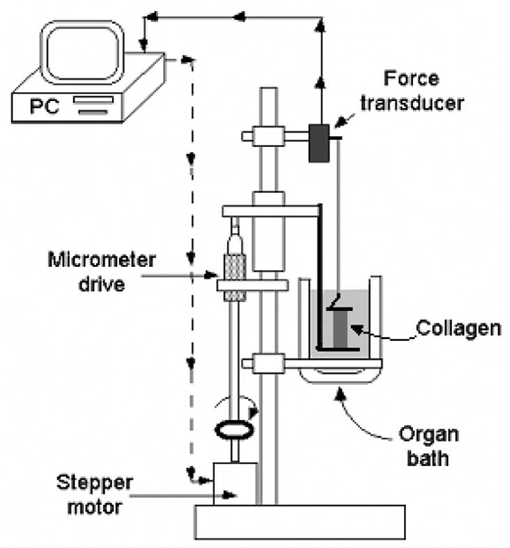
The experimental test apparatus included a temperature-controlled organ bath (Harvard Apparatus, South Natick, MA) and a pair of loading bars controlled by a stepper motor. The fixed bar was suspended from a force transducer (model 52-5945, Harvard Apparatus, South Natick, MA). The lower, movable bar was attached to a sliding element controlled by a stepper motor (P/N 1-19-3400, 24V DC, 1.8° step size, Howard Industry, St. Louis, MO) through a micrometer. The micro-stepping driver (IM483, Intelligent Motion Systems, Inc., Marlborough, CT) was controlled using the “experix” software system developed by William B. McConnaughey (sourceforge.net).

Figure 3.

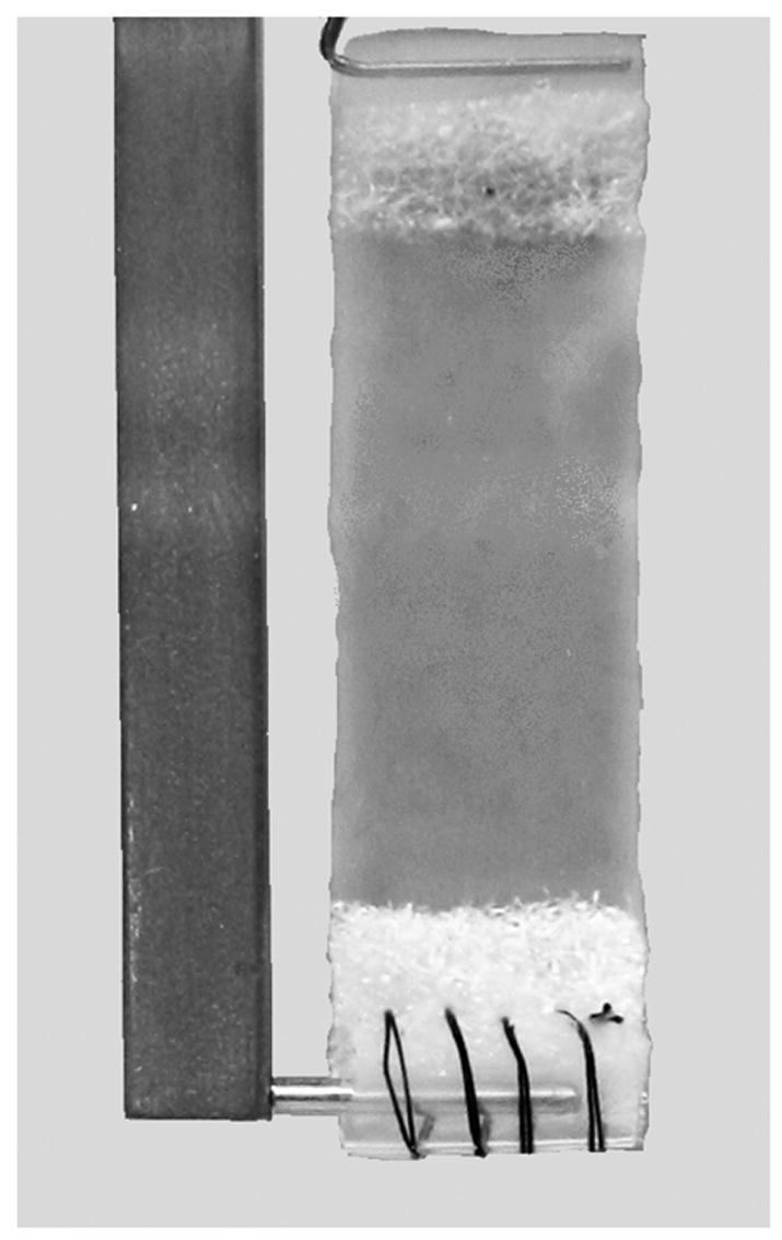
Flat collagen gel specimens were mounted to the testing apparatus via relatively rigid polymer attachments. Specimens were synthesized from 4 mg/ml rat-tail type I collagen stock solution (Upstate Biotechnologies) in 0.02M acetic acid, with pH brought to 7.4 using sodium hydroxide. The solution was poured into rectangular molds and kept in 37°C for 15 hours. The molds contained fabric attachments that were folded and stitched over a plastic tube to facilitate attachment to testing bars. The specimens were approximately 30mm long, 10mm wide, and 3mm thick.

Four specimens were tested in a sequence of “ramp-and-hold” stretches. After adjusting the loading bars until each specimen was at zero stress, specimens were stretched at a prescribed rate over T_R seconds then held for T_H seconds while force was recorded at 10 Hz.

To characterize the strain-dependence of nonlinearity, four consecutive ramp-and-hold tests were performed on each specimen, each involving a stretch of 2.0 mm (stretch λ=1.067) over T_R=20 seconds, and a hold of T_H=2000 seconds, sufficient for specimens to relax to a nearly constant level of force. This loading rate was chosen to ensure that inertial effects could be neglected (Nekouzadeh, et al., 2005).

This protocol was applied three more times until the specimens were stretched 8.0 mm (λ=1.267). After the final ramp-and-hold increment, the loading bars were returned to their pre-test separation, and the specimens were allowed to relax for 2000 seconds (an interval sufficient to remove all slack from the specimens). Thereafter, specimens were stretched 8.0 mm at constant rate over T_R=10 seconds to compare the predictive ability of the adaptive and Fung approach for including nonlinearity.

4.2 Calibration of QLV Models

The adaptive QLV model, Fung’s QLV model, and the “generalized Fung” models were calibrated for each specimen from the force relaxation data in each “hold” of the incremental ramp-and-hold tests; force data in the “ramps” were used to evaluate the models’ predictive ability. Details of the calibration procedures are provided in the supplementary online document.

Briefly, in all cases g(t) was assigned an exponential form with time constants τ_i. Therefore, isometric (“hold”) force relaxation data h(t) could be written as a linear combination of the exponential terms comprising g(t):

$$h(t)=c_o+\underset{i}{\Sigma }{c}_i{e}^{-t/{\tau }_i}.$$

An interesting advantage of expressing g(t) with exponential terms is that this enables us to find the time constants directly from the hold data. For each dataset, fitting h(t) required a four-term exponential summation (including one infinite time constant).

4.3 Reloading

To study re-stretched specimens, inelastic deformation had to be considered. The inelastic behavior of collagen is not a focus of this paper, and the following scheme was employed only because it was simple and plausible. Strain in Equations (1) and (3) was replaced on reloading with ${\epsilon }_i^p(t)$:

$${\epsilon }_i^p(t)=\{\begin{array}{cc}0& \text{if\hspace{0.17em}}\epsilon <{\epsilon }_i^{\ast }\\ \epsilon (t)-{\epsilon }_i^{\ast }& \text{if\hspace{0.17em}}\epsilon >{\epsilon }_i^{\ast }\end{array}\hspace{0.17em}\hspace{0.17em}\hspace{0.17em}i=0,1,2,\mathrm{....},$$

where ${\epsilon }_i^p$ could be different for different relaxation modes, and ${\epsilon }_i^{\ast }$ were constants fit from the hold data of the large strain test. Choosing independent ${\epsilon }_i^{\ast }$ was based upon the experimental observation that different nonlinear behavior was exhibited at each time scale.

5. Results

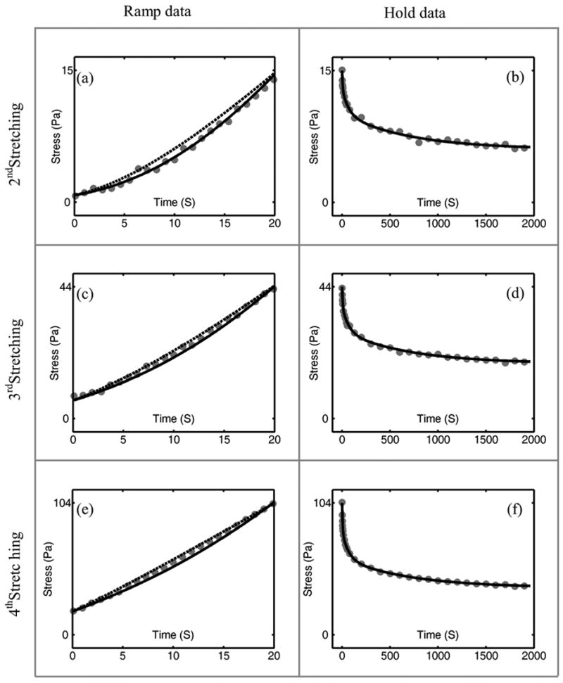
The adaptive QLV model is sufficiently general to fit the calibration data itself, but Fung’s QLV model could do so only to within ~10% due to the model’s limitation that amplitudes of relaxation modes retain the same relative proportions for all strain (right column of Figure 4: Figures 4(b), 4(d) and 4(f)). The fit of the Fung QLV model was forced to capture the initial stress of hold data (stress at the end of the ramp) to provide the best possible prediction of the ramp data; this came at the expense of its predictions at longer timescales. Predictions of the generalized Fung model for the hold data were indistinguishable from those of the adaptive QLV model (Figure 5) and its predictions of the ramp data were very close to those of Fung’s QLV model.

Figure 4.

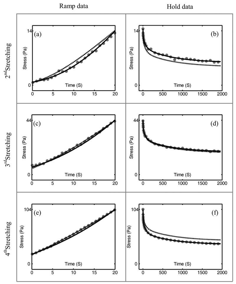
Predictions of the Fung QLV model (dashed lines) compared to those of the adaptive QLV model (solid lines) for incremental ramp and hold data (gray dots) for the second, third and fourth ramp- and-hold tests. The three rows correspond to ramp-and-hold tests from strains of 4.3% to 11% ((a) and (b)), 11% to 17.7% ((c) and (d)) and 17.7% to 24.3% ((e) and (f)). Stress is calculated by dividing the recorded force by 30 mm², the nominal cross-sectional area of the specimens.

Figure 5.

Predictions of the generalized Fung model (dashed lines) compared to those of the adaptive QLV model (solid lines) for incremental ramp and hold data (gray dots) for the second, third and fourth ramp- and-hold tests. As in Figure 4, the three rows correspond to ramp-and-hold tests from strains of 4.3% to 11% ((a) and (b)), 11% to 17.7% ((c) and (d)) and 17.7% to 24.3% ((e) and (f)). Stress is calculated by dividing the recorded force by 30 mm², the nominal cross-sectional area of the specimens.

Predictions of the ramp data serve to evaluate the calibrated models. Ramp loading stress-strain data were concave up (representative incremental stretch data in the left column of Figure 4: 4(a), 4(c), 4(e)), meaning that, for the reconstituted collagen, the effect of nonlinearity is important during a 6.7% strain increment, and the response cannot be approximated with linear viscoelasticity (which predicts a concave down response). Both models predict appropriate concave up behavior (Figure 4) with acceptable accuracy when fit to the hold stress relaxation data. Again, we biased Fung’s QLV model to fit to the ramp at the expense of fitting longer timescale calibration data.

For the adaptive QLV model, the three g_i(t) = e^−t/^τi were exponentials with time constants of τ₁=5.5 sec, τ₂=65.5 sec, and τ₃=700 sec. The corresponding elastic stiffnesses k₁(ε), k₂(ε) and k₃(ε) were clearly not proportional to each other (Figure 6). The curvature of the k(ε) functions (representing the degree of nonlinearity) was lower for the larger time constants. The fit for Fung’s QLV model yielded similar time constants: τ₁=5.9 sec, τ₂=67.5 sec, and τ₃=734 sec. The assumption of piecewise linearity for the elastic stress function was accurate within 10% (Figure 7).

Figure 6.

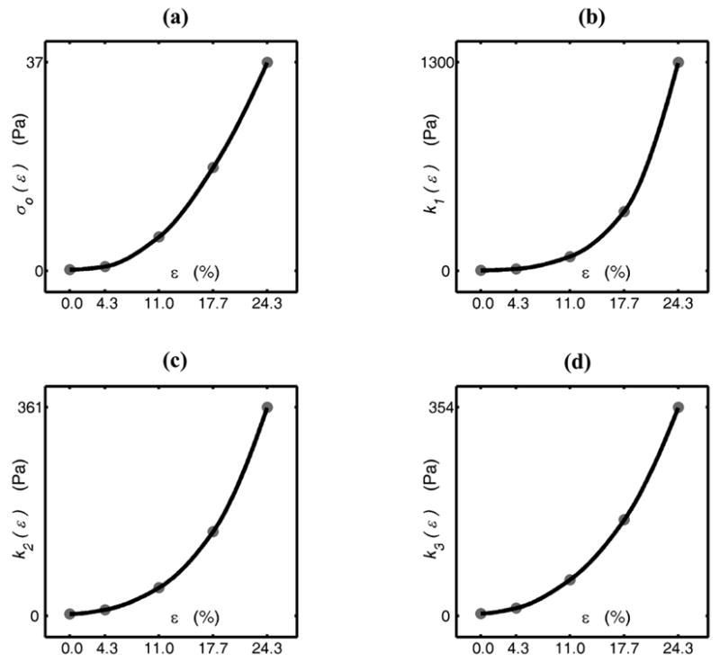
The elastic stress (a) and the elastic stiffnesses of the viscoelastic components of the adaptive QLV model (b, c, and d), as fit to the collagen specimens in 1-D. The gray dots are the calibrated values for k_i (ε) and σ_o (ε), and solid lines represent interpolations for the intermediate strains.

Figure 7.

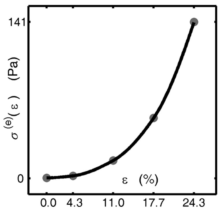
The elastic stress function for Fung’s QLV model, as fit to experimental data. The gray dots are calibrated values, and the solid lines are interpolations (validated with a second iteration of calibration procedure, as described in the supplemental online document).

The adaptive QLV model fit the large strain ramp-and-hold test very well (Figure 8). The recorded stress started to increase visibly after 3 seconds (Figure 8(a)). The generalized Fung model captured only the first 6 seconds of the response. By altering ${\epsilon }_i^{\ast }$, the generalized Fung model could instead be forced to capture the peak stress at the end of loading at the expense of losing the fit to the initial stress rise.

Figure 8.

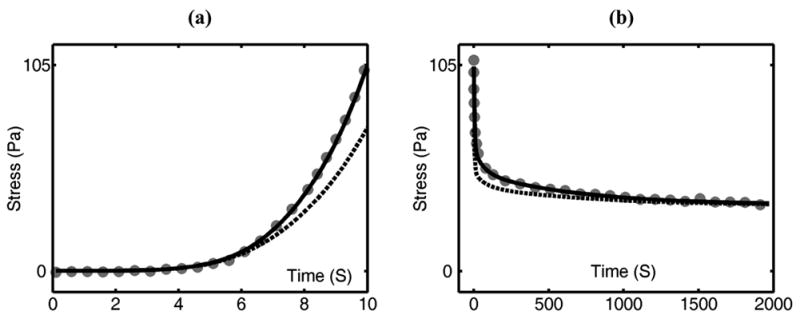
Predictions of the adaptive QLV model (solid lines) and generalized Fung model (dotted lines) of large strain ramp-and-hold test (data: gray dots). The time axis for the ramp (a) can be converted to strain using the stretch rate of 0.8 mm/s and the reference length of 30 mm. The optimum values of ${\epsilon }_i^{\ast }$ used in both models were ${\epsilon }_0^{\ast }=4.5\%$, ${\epsilon }_1^{\ast }=8.3\%$, ${\epsilon }_2^{\ast }=12.8\%$ and ${\epsilon }_3^{\ast }=11.7\%$

6. Discussion

The adaptive QLV model presented in this paper adapts all stress relaxation from the strain history to the material conditions at the current strain level. The model possesses extra degrees of freedom compared to Fung’s QLV model, enabling it to capture non-proportionality in the relaxation curves at different strains.

To separate the merits of the two approaches for incorporating quasi-linearity from those of allowing extra degrees of freedom, we compared predictions of the adaptive QLV and generalized Fung models. The distinction between the two approaches is negligible when stretching is small, as both models can be approximated with piecewise linear viscoelasticity for small stretching.

However, the difference was magnified in a test involving a large stretch. The protocol was to calibrate both models at multiple strain levels over a prescribed range, and then, using a model for inelastic deformation, compare predictions of the calibrated models to data from a subsequent stretch over this entire strain range. Although both calibrated models provided similar, accurate predictions during incremental steps (Figure 5), the adaptive QLV model captured the significantly larger curvature over the ramp portion of the test, but the generalized Fung model could not (Figure 8). As the strain increased during the ramp, the adaptive QLV model adapted the relaxation functions from the strain history to current strain levels, providing appropriate magnification of the nonlinearity and leading to a more accurate prediction of the increased curvature. Models based upon the approach of the Fung QLV model cannot capture this.

From a modeling perspective, the adaptive QLV model is easier to calibrate and use than the Fung QLV model or its generalized version, especially when the input stretch for calibration is not a step function. Calibration involves finding the strain dependent amplitudes (k_i(ε), A_i(ε) and σ^(e)(ε)) and is simple because the unknown nonlinear function of strain lies outside the convolution integral. This is far less involved than fitting a function inside a convolution integral, as is required for Fung’s QLV model.

As an example, consider a single large strain ramp-and-hold test to be modeled with a QLV model, and assume that proportionality at different strains is not an issue so that we may obtain an accurate representation of material response with either the Fung model or the single term adaptive QLV model. Time constants can be found from the exponential fit to the hold data. In the adaptive approach the amplitudes of the reduced relaxation function are known scales of the amplitudes of the exponential fit to the hold data (Equation (S2) in the supplementary online document, with only one k(ε)). V^(ε)(t) is calculated from the reduced relaxation function, and k(ε(t)) is determined by simply dividing σ(t) by V^(ε)(t) during the ramp. In the Fung approach, determining the amplitudes of the reduced relaxation function from amplitudes of the exponential fit to the hold data requires prior knowledge of σ^(e)(ε). Also, determining σ^(e)(ε) from stress during the ramp requires prior knowledge of the amplitudes of the reduced relaxation function. Therefore the model parameters must be found from iterative solution of coupled nonlinear equations, an optimization problem for finding one function and a few scalars. Additionally, for each choice of the amplitudes of the reduced relaxation function, σ^(e)(ε) must be found from a numerical deconvolution. Further details of the calibration procedures and the simplicity of the adaptive QLV approach for multiple tests at different strain levels are described in the supplementary online document.

References

- Abramowitch SD, Woo SL. Bioengineering Conference. Sonesta Beach Resort in Key Biscayne; Florida: 2003. A New Analytical Approach to Evaluate the Viscoelastic Properties of the Goat Medial Colateral Ligament Using the Quasi-Linear Viscoelastic Theory. [Google Scholar]
- Alberts B, Bray D, Lewis J, Raff M, Roberts K, Watson JD. Molecular Biology of the Cell. New York: Garland; 1994. [Google Scholar]
- Christiansen DL, Huang EK, Silver FH. Assembly of type I collagen: Fusion of fibril subunits and the influence of fibril diameter on mechanical properties. Matrix Biol. 2000;19:409–420. doi: 10.1016/s0945-053x(00)00089-5. [DOI] [PubMed] [Google Scholar]
- Coleman BD, Noll W. Foundation of Linear Viscoelasticity. Review of Modern Physics. 1961;33:239–149. [Google Scholar]
- Decraemer WF, Maes MA, Vanhuyse VJ, Vanpeperstraete P. A non-linear viscoelastic constitutive equation for soft biological tissues, based upon a structural model. J Biomech. 1980;13:559–64. doi: 10.1016/0021-9290(80)90056-1. [DOI] [PubMed] [Google Scholar]
- Fung YC. Biomechaics: Mechanical Properties of Living Tisues. New York: Springer; 1993. [Google Scholar]
- Hsu S, Jamieson A, Blackwell J. Viscoelastic studies of extracellular matrix interactions in a model native collagen gel system. Biorheology. 1994;31:21–36. doi: 10.3233/bir-1994-31103. [DOI] [PubMed] [Google Scholar]
- Johnson GA, Livesay GA, Woo SL, Rajagopal KR. A single integral finite strain viscoelastic model of ligaments and tendons. J Biomech Eng. 1996;118:221–6. doi: 10.1115/1.2795963. [DOI] [PubMed] [Google Scholar]
- Lanir Y. Constitutive equations for the lung tissue. J Biomech Eng. 1983;105:374–80. doi: 10.1115/1.3138435. [DOI] [PubMed] [Google Scholar]
- Misof K, Rapp G, Fratzl P. A new molecular model for collagen elasticity based on synchrotron X-ray scattering evidence. Biophysical Journal. 1997;72:1376–1381. doi: 10.1016/S0006-3495(97)78783-6. [DOI] [PMC free article] [PubMed] [Google Scholar]
- Neubert HKP. A simple model representing internal damping in solid materials. Aeronautical Quarterly. 1963;14:187–210. [Google Scholar]
- Ozerdem B, Tozeren A. Physical response of collagen gels to tensile strain. J Biomech Eng. 1995;117:397–401. doi: 10.1115/1.2794198. [DOI] [PubMed] [Google Scholar]
- Parry D. The molecular and fibrillar structure of collagen and its relationship to the mechanical properties of connective tissue. Biophys Chem. 1988;29:195–209. doi: 10.1016/0301-4622(88)87039-x. [DOI] [PubMed] [Google Scholar]
- Pins GD, Christiansen DL, Patel R, Silver FH. Self-assembly of collagen fibers. Influence of fibrillar alignment and decorin on mechanical properties. Biophysical Journal. 1997;73:2164–2172. doi: 10.1016/S0006-3495(97)78247-X. [DOI] [PMC free article] [PubMed] [Google Scholar]
- Pioletti DP, Rakotomanana LR, Benvenuti JF, Leyvraz PF. Viscoelastic constitutive law in large deformations: application to human knee ligaments and tendons. J Biomech. 1998;31:753–7. doi: 10.1016/s0021-9290(98)00077-3. [DOI] [PubMed] [Google Scholar]
- Provenzano P, Lakes R, Keenan T, Vanderby R., Jr Nonlinear ligament viscoelasticity. Ann Biomed Eng. 2001;29:908–14. doi: 10.1114/1.1408926. [DOI] [PubMed] [Google Scholar]
- Provenzano PP, Lakes RS, Corr DT, R R., Jr Application of nonlinear viscoelastic models to describe ligament behavior. Biomech Model Mechanobiol. 2002;1:45–57. doi: 10.1007/s10237-002-0004-1. [DOI] [PubMed] [Google Scholar]
- Pryse K, Nekouzadeh A, Genin G, Elson E, Zahalak G. Incremental mechanics of collagen gels: new experiments and a new viscoelastic model. Ann Biomed Eng. 2003;31:1287–96. doi: 10.1114/1.1615571. [DOI] [PubMed] [Google Scholar]
- Sacks MS. Incorporation of experimentally-derived fiber orientation into a structural constitutive model for planar collagenous tissues. J Biomech Eng. 2003;125:280–287. doi: 10.1115/1.1544508. [DOI] [PubMed] [Google Scholar]
- Silver FH, Christiansen DL, Snowhill PB, Chen Y. Transition from viscous to elastic-based dependency of mechanical properties of self-assembled type I collagen fibers. Appl Polym SCi. 2000;79:134–142. [Google Scholar]
- Thomopoulos S, Marquez JP, Weinberger B, Birman V, Genin GM. Collagen fiber orientation at the tendon to bone insertion and its influence on stress concentrations. J Biomech. 2006;39:1842–51. doi: 10.1016/j.jbiomech.2005.05.021. [DOI] [PubMed] [Google Scholar]
- Thornton GM, Frank CBGSN. Ligament creep behavior can be predicted from stress relaxation by incorporating fiber recruitment. J Rheol. 2001;45:493–507. [Google Scholar]
- Wagenseil JE, Wakatsuki T, Okamoto RJ, Zahalak GI, Elson EL. One-dimensional viscoelastic behavior of fibroblast-populated collagen matrices. J Biomech Eng. 2003;125:719–725. doi: 10.1115/1.1614818. [DOI] [PubMed] [Google Scholar]
Associated Data
This section collects any data citations, data availability statements, or supplementary materials included in this article.