Forty mouse strain survey of voluntary calcium intake, blood calcium, and bone mineral content

Abstract

We measured voluntary calcium intake, blood calcium, and bone mineral content of male and female mice from 40 inbred strains. Calcium intakes were assessed using 48-h two-bottle tests with a choice between water and one of the following: water, 7.5, 25, and 75 mM CaCl₂, then 7.5, 25, and 75 mM calcium lactate (CaLa). Intakes were affected by strain, sex, anion, and concentration. In 11 strains females consumed more calcium than did males and in the remaining 29 strains there were no sex differences. Nine strains drank more CaLa than CaCl₂ whereas only one strain (JF1/Ms) drank more CaCl₂ than CaLa. Some strains had consistently high calcium intakes and preferred all calcium solutions relative to water (e.g., PWK/PhJ, BTBR T⁺tf/J, JF1/Ms). Others had consistently low calcium intakes and avoided all calcium solutions relative to water (e.g., KK/H1J, C57BL/10J, CE/J, C58/J). After behavioral tests, blood was sampled and assayed for pH, ionized calcium concentration, and plasma total calcium concentration. Bone mineral density and content were assessed by DEXA. There were no significant correlations between any of these physiological measures and calcium intake. However, strains of mice that had the highest calcium intakes generally fell at the extremes of the physiological distributions. We conclude that the avidity for calcium is determined by different genetic architecture and thus different physiological mechanisms in different strains.

Adequate calcium intake is essential for many physiological processes but the controls of calcium intake are not well understood [reviews [45,54]]. Blood ionized calcium may regulate calcium intake [30,51,54], perhaps by acting on calcium receptors in the brain [e.g., [32]]. Circulating levels of parathyroid hormone, calcitonin, and 1,25-dihydroxyvitamin D influence calcium intake [e.g., [12,30,43,51,61]] but it is unclear whether these effects are due to the direct action of the hormones on the brain or to their indirect actions on blood calcium levels. The most-studied control of calcium intake involves orosensory acceptance. Calcium deficiency lowers the behavioral and electrophysiological detection thresholds for calcium [25]. It also increases the avidity for concentrations of calcium that are disliked in the replete state: calcium deficiency increases calcium intakes in preference tests [14,25], the rate of sham-ingestion of calcium [34], the frequency of hedonically positive facial expressions during calcium consumption [33], and the response to oral calcium of sweet-best units in the nucleus of the solitary tract [35]. Ingestion or infusion of calcium can also condition preferences for arbitrary flavors [13,23,24,55]. Taken together, these findings argue that the oral modulation of calcium acceptance plays an important role in governing calcium consumption.

Animals consume calcium solutions even when calcium is available in adequate amounts in the diet. This “need-free”, “spontaneous”, or “voluntary” intake is dependent on several factors such as age or growth rates, sex, diet, and the type and form of calcium available [review [54]]. Even less is known about the controls of this behavior than deficiency-related calcium appetite, although the assumption is that calcium-replete animals consume calcium because they “like” it, and this is mediated by taste.

Given the slow progress and the complexity of physiological analysis in this area of research it seemed appropriate to try other approaches. To this end, we have begun to investigate the genetic basis of calcium intake and appetite. An important first step toward conducting genetic analyses is to find strains with diverse phenotypes. In a previous paper, we reported the voluntary intakes and preferences of a range of concentrations of CaCl₂ by male mice from 28 inbred strains [1]. Here, we present a more comprehensive survey. We measured the preference for CaCl₂ and calcium lactate (CaLa) of male and female mice of the 40 strains forming the core of the Mouse Phenome Project, which is a repository of phenotypic information from inbred mouse strains [49]. To hunt for relationships between calcium consumption and underlying physiology, we also measured blood ionized and total calcium concentrations, and bone mineral density and content. Accompanying papers report other measures collected from these mice, including voluntary intake of water and sodium solutions [62] and body composition [40].

1. Methods

1.1. Mice

A total of 790 mice, comprising approximately 10 males and 10 females from 40 strains [50] were tested in five squads of 188, 170, 135, 186, and 111 mice, conducted over a 12-month period in October 2001–2002. The mice were bred by The Jackson Laboratory and shipped to our institution when ~8 wk old. A few mice were slightly younger or older because of supply problems [see [56,57] for details of exact ages, and which mice were assigned to which squad].

While at The Jackson Laboratories, the mice were housed in same-strain, same-sex groups and fed Purina 5K52 or 5K54 diet. After they arrived at our institution, they were individually housed in plastic “tub” cages and fed AIN-76A diet. This is a semisynthetic diet containing by weight: 20% protein (casein), 65% carbohydrate (sucrose and cornstarch), 5% fat (corn oil), and 10% fiber (cellulose), minerals and vitamins. It contains 0.13 mmol/g Ca²⁺ and has an energy content of ~15.9 kJ/g [Dyets, cat. No 100000; [19]]. When mice were not being tested, deionized water was available from an inverted 300-mL glass bottle with a rubber stopper and stainless steel drinking spout. Cages were changed every 4 days (between 48-h tests). The vivarium was maintained at 23 °C on a 12:12 h light/dark cycle with lights off at 7 pm. A detailed description of mouse husbandry, housing conditions, and other procedures, including drinking tube construction, is available on-line [56,57]. Abbreviated details are given below.

1.2. Procedures

1.2.1. Taste preference tests

After 6–10 days to habituate to laboratory conditions, all mice received a series of two-bottle choice tests. Seven 48-h two-bottle choice tests were conducted in the following order: water, 7.5, 25, and 75 mM CaCl₂, 7.5, 25, and 75 mM CaLa. For the “water” test, the mice received two tubes of deionized water. For the other tests, the mice received a choice between water and the compound listed. The CaCl₂ was purchased from Sigma Chemical Corp. and the CaLa from Fisher Scientific. Both were dissolved in deionized water. Their concentrations were chosen based on previous work in rats [e.g., [53]] and mice [1] with the aim of spanning the range from indifference to strong avoidance. After the tests with calcium salts, all the mice were tested with three concentrations each of NaCl and sodium lactate, as described elsewhere [62]. Body weight was measured (to the nearest 0.1 g) at the beginning and end of the test series.

Because some strains of mice prefer to drink from the tube on their left [2,59] tube position was switched every 24 h. For the first day of each test, the calcium solution was presented on the mouse’s left and on the second day it was presented on the right. Intakes were measured to the nearest 0.2 mL at the end of each test by reading the position of the fluid meniscus against a graduated scale. Fluid spillage and evaporation were ignored in this experiment. Previous work with identical procedures indicates they account for <0.5 mL over 48 h [58,60]. Occasionally, data were lost due to spilled drinking tubes or other technical problems. In these cases, the mice were re-tested at the end of the series.

1.2.2. Blood calcium

At 5–9 days after the end of behavioral tests, blood ionized calcium, blood pH and plasma total calcium were measured in awake mice. Samples were collected between 10 am and 2 pm, in the middle of the light period, with mice from different strains sampled in a counterbalanced order to control for any effects due to time of day. Each mouse was placed on a flat surface and restrained by hand or with a towel. The tip of the mouse’s tail was removed with a scalpel, and ~40 µL blood was gently “milked” into two 100-µL glass, heparinized microhematocrit tubes (Fisher brand). Pilot work determined that under the conditions used here, the heparin coating of the microhematocrit tubes has little effect on calcium concentrations.

One of the two samples collected from each mouse was analyzed for blood ionized calcium and pH using a clinical ionspecific electrode (Dow Corning 634 calcium analyzer). Blood ionized calcium levels are highly sensitive to pH. To avoid changes in pH due to contamination by atmospheric CO₂, the analyzer was located in the vivarium so that samples could be analyzed immediately after they were collected (within 15 s). In addition, we used a stopwatch to measure the time between when the mouse was removed from its cage and when the first tube of blood was collected. Ionized calcium concentrations were adjusted for pH using a standard formula [11].

The other sample was centrifuged and resulting plasma analyzed for total calcium using a colorimetric method (Sigma Chemical Corp., kit no. 587) that was miniaturized to use 2.5 µl plasma and a 96-well plate format. Three of the 790 plasma total calcium samples were lost due to a technical error.

1.2.3. Bone mineral density and content

Exactly 1 wk after the blood calcium sample, at which time the mice were ~16 wk old, each mouse was anesthetized with 70 mg/kg ketamine+10 mg/kg xylazine (5 ml/kg, i.p.) and as much blood as possible (400–1400 µL) removed by cardiac puncture (for another experiment). The dead mouse was then wrapped in aluminum foil and frozen at −80 °C. Several months later, frozen carcasses were allowed to thaw at room temperature for ~1 h and were then analyzed using a PIXIMus II mouse densitometer (#51601; GE Medical Systems Lunar, Madison, WI). The PIXImus II uses low energy X-rays to produce high-resolution (0.18 × 0.18 mm pixel) images. Software included with the machine estimates bone mineral density (BMD; mg/cm²) and content (BMC, g; as well as the weight of lean and fat tissue, which will not be reported here).

Each carcass was laid in the prone position on a plastic tray. The limbs were held splayed apart with tape. The tail was displaced to the mouse’s left so that it was within the X-ray field but did not overlap a limb. Because the cone-beam X-ray field is only 80 × 65 mm and thus too small to fit a large adult mouse, the head of each mouse was excluded from analysis; it was either placed outside the X-ray field or masked using software. The PIXIMus II was calibrated daily using a plastic “mouse phantom” provided by the manufacturer.

To provide an index of the reliability of the PIXIMus II, 160 carcasses (two from each sex of each strain, chosen randomly) were reanalyzed after freezing and re-thawing several weeks later. The correlation between the first and second analysis was r=0.93 for BMD and r=0.97 for BMC.

1.3. Data analysis

1.3.1. Measures of consumption

Intakes from 48 h tests were divided by two to provide average daily intakes. To account for differences in body size among the strains (Table 1), all fluid intakes were adjusted in relation to body surface (i.e., mL/kg BW^0.667). A detailed justification and caveats of this approach is provided elsewhere [62]. Preference scores were calculated based on solution intake/(solution intake+water intake) × 100.

Table 1.

Correlation matrix of calcium solution intakes and preferences for 40 strains of mice

	7.5mM Cacl2	25mM CaCl2	75mM CaCl2	7.5mM CaLa	25mM CaLa	75mM CaLa	BW
7.5mM Cacl2	0.63	0.89	0.65	0.88	0.84	0.81	−0.21
25mM CaCl2	0.81	0.81	0.82	0.88	0.90	0.88	−0.28
75mM CaCl2	0.44	0.73	0.93	0.60	0.70	0.81	−0.20
7.5mM CaLa	0.73	0.79	0.40	0.74	0.95	0.85	−0.14
25mM CaLa	0.73	0.86	0.53	0.87	0.75	0.93	−0.16
75mM CaLa	0.70	0.89	0.70	0.76	0.91	0.83	−0.10
Water	0.18	0.18	−0.13	0.23	0.19	0.12	0.06
Body weight	−0.16	−0.22	−0.20	−0.20	−0.23	−0.16
	Intakes adjusted for body weight0.667

Values are Pearson correlation coefficients based on 40 means from each strain (both sexes combined). Correlations between intakes adjusted for body weight^0.667 are shown at bottom left, correlations between preferences are shown top right. The top-left to bottom-right diagonal (in yellow) shows correlations between intake and preference. Values outlined in green show correlations between identical concentrations of CaCl₂ and calcium lactate (CaLa). Bold=significant at p<0.01 level. Water = total water intake from two tubes. BW=body weight at start of two-bottle tests.

To determine the consistency between adjusted calcium intakes and preference scores, we calculated the Pearson correlation coefficients between adjusted intakes and preferences based on the 80 means (40 strains × 2 sexes) for each of the 6 taste solution tests. The correlations were relatively high for five of the six tests of calcium ingestion (r’s=0.74–0.93; Table 1). The correlation between 7.5 mM CaCl₂ intake and preference was lower (r=0.63), perhaps because some strains may not have been able to taste it. It is sometimes appropriate to adjust preference scores with an arcsine-root transformation in order to achieve sample normality but this only marginally increased the strength of correlations (data not shown).

We considered the correlations between adjusted intakes and preferences for calcium choice tests to be high enough that it would be redundant to present the results of both dependent variables, and so here present only one measure. We chose to present adjusted intakes because calcium preference data are available elsewhere [57] but adjusted intakes are not.

1.3.2. Statistical analyses

Body weight-adjusted intakes of calcium were analyzed in an omnibus ANOVA with factors of Strain, Sex, Anion and Concentration. Additional analyses of water intake and total fluid intake during taste solution tests were also conducted but revealed little of interest so are not described here. Similar ANOVAs (i.e., with factors of Strain and Sex) were used to analyze each of the physiological measures collected.

Several of the analyses produced complex interactions so more focused analyses were conducted. To determine differences between strains in calcium intake, we conducted post hoc analyses of the omnibus ANOVAs using Tukey's tests to reveal “homogenous” groups with statistically similar means [see [1,2] for examples of this approach]. However, for some measures in this experiment there were 15 or more overlapping homogenous groups that were hard to describe concisely, and of little value for subsequent interpretation. To provide a more concise and simple identification of outlying strains, we calculated 95% confidence intervals based on the overall mean of the 40 strain means (i.e., overall mean±1.96 × standard error of the means), and used these as a criterion to recognize strains with unusually high or low phenotypes.

To determine effects within each strain, a series of 40 mixed-design ANOVAs involving Sex, Anion and Concentration were conducted. In essence, for these analyses, the results from each strain were treated as if they had been generated in separate, independent experiments. Tukey’s post hoc tests were used to determine whether differences existed between individual pairs of means. For all tests, the criterion for significance was p<0.01.

2. Results

2.1. Body weight

At the beginning of the taste preference tests there were highly significant differences among the strains in body weight and in most, but not all, cases males were significantly heavier than females. These differences persisted throughout the preference test period [see [62] for details].

2.2. Comparison of CaCl₂ and CaLa intake

Initial inspection of the results suggested that strains with high intakes of a particular concentration of CaCl₂ also had high intakes of the same concentration of CaLa. To investigate the degree of this relationship in detail, we compared intakes of each strain and sex in scatter plots (Fig. 1). Correlation coefficients for individual concentrations are given in Table 1. The linear regression equation between CaCl₂ and CaLa intakes for all three concentrations was given by the formula, CaLa intake=0.71 × CaCl₂ intake+8.6 (r=0.75, n=240).

Fig. 1.

Scatter plot of intake of three concentrations of CaCl₂ versus calcium lactate (CaLa; r=0.75). Each point represents the mean value of ~10 mice of the same sex and strain. The four outlying high points are all from the MSM/MsJ strain. The outlying low point is from C58/J females given 7.5 mM concentrations.

Although there were strong correlations between chloride and lactate intakes there were also sufficient numbers of outliers that we considered it inappropriate to ignore the anion when describing the results. As a compromise between detailed presentation and thrifty use of journal space, we describe the results with individual anions when making within-strain comparisons but use averages of the chloride and lactate intakes when making between-strain comparisons.

2.3. Within-strain comparisons of calcium intake

Below are summarized the results of ANOVAs based on calcium intakes of each strain analyzed individually. Fig. 2 shows the means and standard errors of the mean for each sex, anion, and concentration tested.

Fig. 2.

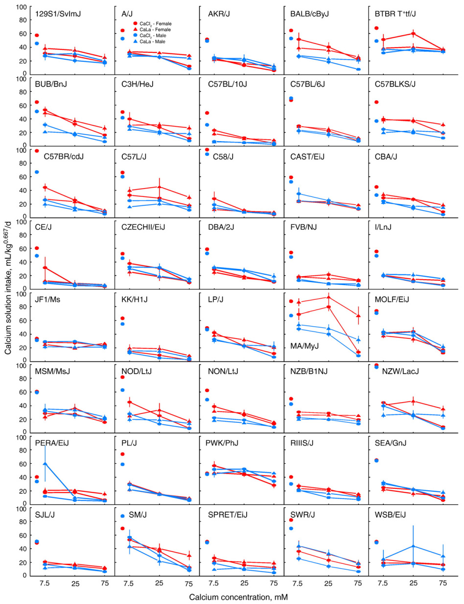
Mean CaCl₂ (circles) and CaLa (triangles) intakes (adjusted for bodyweight^0.667) of male (blue) and female (red) mice from 40 strains. Free-standing circles are total water intakes in two-bottle water versus water test. Water intakes for C58/J females (126 mL/kg^0.667) and NZW/LacJ males (139 mL/kg^0.667) are drawn at top of scale because they fall outside range of graph. Vertical lines are standard errors of the mean; these are smaller than the symbols in most cases.

2.3.1. Sex × anion × concentration

There were no significant three-way interactions for any of the 40 ANOVAs conducted.

2.3.2. Sex × anion

BALB/cByJ, BTBR T⁺tf/J, and C57L/J showed an interaction of sex × anion on intake. For BALB/cByJ and BTBR T⁺tf/J, this was because females drank more CaCl₂ than did males but the two sexes drank similar amounts of CaLa. For C57L/J, this was because females drank more CaLa than did males but the two sexes drank similar amounts of CaCl₂.

2.3.3. Anion × concentration

There were two-way interactions between anion × concentration for 24 strains. In every case except one, this was because the mice drank more and had stronger preferences for one or more concentration of CaLa than CaCl₂. The exception was the JF1/Ms strain, which drank more of the two lowest concentrations of CaCl₂ than CaLa but did not differ at the highest concentration.

2.3.4. Sex × concentration

The following strains showed a sex × concentration interaction: BTBR T⁺tf/J, C57BL/10J, CBA/J, FVB/NJ, MA/MyJ, and NON/LtJ. For BTBR T⁺tf/J, C57BL/10J, CBA/J, and MA/MyJ this was because females drank more and had higher preferences for 7.5 and 25 mM calcium solutions than did males, but the two sexes did not differ in 75 mM calcium solution intake or preferences. For FVB/NJ, the two sexes did not differ in intake of 7.5 mM calcium solutions but females drank more 25 and 75 mM calcium solutions than did males.

2.3.5. Sex

Calcium intake was higher in females than males of the following strains: BALB/cByJ, BUB/BnJ, C3H/HeJ, C57BL/10J, C57BLKS/J, C57L/J, CBA/J, MA/MyJ, NON/LtJ, NZB/B1NJ and SPRET/EiJ. Males never drank significantly more calcium than did females of the same strain.

2.3.6. Anion

The following strains drank more CaLa than CaCl₂: 129S1/SvImJ, A/J, BTBR T⁺tf/J, CBA/J, I/LnJ, KK/H1J, MA/MyJ, NZW/LacJ, and SWR/J. The JF1/Ms strain had higher intakes of CaCl₂ than CaLa.

2.3.7. Concentration

Concentration had significant effects on intake in all strains except JF1/Ms and WSB/EiJ.

2.4. Calcium preference, avoidance, and indifference

Table 2 presents calcium preference scores for each mouse strain. A preference score of 50% indicates that a mouse either cannot detect or is indifferent to a taste solution. To determine whether each strain responded to taste solutions with anything other than indifference, mean strain preferences (for both sexes combined) were compared to 50% using one-sample t-tests (Table 2).

Table 2.

Preferences and avoidance of NaCl and NaLa by 40 strains of mice

	CaCl2			CaLa
Strain	7.5 mM	25 mM	75 mM	7.5 mM	25 mM	75 mM
129S1/SvImJ	50±4	43±4↓	31±4↓	58±4	57±5	39±4↓
A/J	51±3	45±3	19±1↓	53±3	52±2	48±2
AKR/J	49±3	35±3↓	14±2↓	42±4↓	38±4↓	25±4↓
BALB/cByJ	59±3↑	47±3	25±3↓	61±3↑	52±4	44±4
BTBR T+tf/J	57±3↑	69±2↑	59±4↑	62±3↑	66±4↑	61±4↑
BUB/BnJ	60±3↑	39±4↓	20±2↓	53±3	49±3	35±3↓
C3H/HeJ	64±4↑	53±4	23±2↓	64±3↑	56±4	50±5
C57BL/10J	34±3↓	21±2↓	9±1↓	29±3↓	24±3↓	18±2↓
C57BL/6J	39±2↓	30±2↓	11±1↓	42±2↓	34±2↓	19±1↓
C57BLKS/J	48±2	43±1↓	27±3↓	45±2↓	49±2	43±2↓
C57BR/cdJ	36±1↓	20±2↓	7±0↓	24±2↓	17±2↓	12±1↓
C57 L/J	43±2↓	37±3↓	23±2↓	40±3↓	41±3↓	34±3↓
C58/J	25±5↓	8±1↓	5±0↓	11±2↓	7±1↓	6±0↓
CAST/EiJ	44±3↓	40±4↓	22±2↓	42±2↓	40±2↓	30±2↓
CBA/J	61±3↑	45±5	16±1↓	58±3↑	52±3	40±4↓
CE/J	27±5↓	11±1↓	8±1↓	22±4↓	15±3↓	11±1↓
CZECHII/EiJ	60±4↑	55±6	22±3↓	49±6	38±6↓	22±3↓
DBA/2J	52±3	42±4↓	20±2↓	51±3	40±3↓	29±4↓
FVB/NJ	31±3↓	27±4↓	19±2↓	33±4↓	24±3↓	21±3↓
I/LnJ	33±2↓	21±1↓	11±0↓	38±3↓	36±3↓	27±2↓
JF1/Ms	68±2↑	69±3↑	57±2↑	57±4↑	56±4↑	59±3↑
KK/H1J	24±3↓	12±2↓	3±0↓	28±4↓	25±4↓	11±1↓
LP/J	71±3↑	48±5	20±3↓	65±4↑	61±4↑	39±4↓
MA/MyJ	65±3↑	62±3↑	13±2↓	77±2↑	74±4↑	54±6
MOLF/EiJ	56±3	57±3	21±2↓	58±2↑	56±4	32±5↓
MSM/MsJ	51±4	50±5	34±3↓	48±5	52±5	36±5↓
NOD/LtJ	45±3	24±3↓	9±0↓	32±4↓	31±4↓	22±3↓
NON/LtJ	47±1	39±2↓	23±4↓	41±2↓	37±2↓	25±2↓
NZB/B1NJ	53±1	47±1	33±2↓	48±1	46±1↓	42±3↓
NZW/LacJ	37±2↓	24±2↓	9±1↓	38±3↓	41±4↓	38±4↓
PERA/EiJ	37±4↓	34±5↓	17±3↓	51±5	42±4↓	29±4↓
PL/J	41±3↓	23±3↓	9±0↓	34±3↓	22±2↓	13±1↓
PWK/PhJ	83±1↑	80±2↑	64±4↑	78±4↑	84±3↑	80±2↑
RIIIS/J	60±2↑	41±3↓	27±3↓	56±2↑	53±3	38±2↓
SEA/GnJ	39±3↓	32±2↓	12±1↓	37±3↓	30±3↓	23±3↓
SJL/J	37±3↓	24±2↓	18±2↓	31±4↓	30±3↓	20±2↓
SM/J	63±4↑	43±5↓	15±2↓	52±6	41±6↓	32±6↓
SPRET/EiJ	46±6	25±4↓	17±3↓	38±4↓	33±5↓	29±3↓
SWR/J	37±3↓	27±3↓	13±1↓	53±4	42±4↓	26±3↓
WSB/EiJ	32±3↓	34±4↓	20±3↓	33±3↓	38±4↓	23±2↓

Values are preference scores (%; i.e., calcium solution intake/total fluid intake × 100) based on intakes of male and female mice combined.

^↑p<0.01, preference score of strain significantly higher than indifference (50%).

^↓p<0.01, preference score of strain significantly lower than indifference (50%).

2.5. Between-strain comparisons

Fig. 3 shows daily intakes of each strain irrespective of anion and sex. There were 5 strains that had mean intakes above the 95% confidence interval for all three concentrations of calcium: BALB/cByJ, BTBR T⁺tf/J, MA/MyJ, NZW/LacJ and PWK/PhJ. There were 11 strains that had mean intakes below the 95% confidence interval for all three concentrations of calcium: AKR/J, C57BL/6J, C57BL/10J, C58/J, CE/J, FVB/NJ, I/LnJ, KK/H1J, SJL/J, PL/J and RIIIS/J.

Fig. 3.

Daily intake of three concentrations of calcium by 40 strains of mice (sexes and anion combined). Strains are arranged in order from lowest to highest intake (adjusted for body weight^0.667) of 75 mM Ca²⁺. The scale for the 25 mM calcium concentrations is offset to improve readability. Vertical shaded bars are 95% confidence intervals from the overall mean for each calcium concentration. Horizontal lines are standard errors of the mean; these are smaller than the symbols in most cases.

2.6. Blood sampling, calcium and pH

There was a strain × sex interaction in blood ionized calcium values, F(39, 712)=1.65, p=0.0087, but the source of this interaction was complex; there were no differences between males and females of the same strain. Overall, males had a statistically significantly lower blood pH than did females, F(1,712)=10.0, p=0.0016, although the difference was so small as to be of no physiological significance (males, 7.193±0.003 (n=395); females, 7.206±0.003 (n=397). There were also effects of sex on total calcium concentrations, F(1,709)=6.76, p=0.0095, but once again, the difference was very small in physiological terms (males, 2.347±0.007 mmol/L; females, 2.371±0.007 mmol/L). All other analyses involving sex were nonsignificant. Consequently, we combined sexes for comparisons between strains.

It was easier to obtain blood from some strains of mice than others (Fig. 4). Some of this discrepancy was due to differences in the ease of restraining the mice but the large majority of the variation was due to difficulty with “milking” blood from the tail. There was no relationship between body weight and the time required to collect blood (r=−0.15, n=40); it was equally easy to handle and bleed small or large mice. The time required to collect blood was independent of blood ionized calcium (r=−0.03, n=40), blood pH (r=0.02, n=40) and plasma total calcium (r=−0.03, n=40).

Fig. 4.

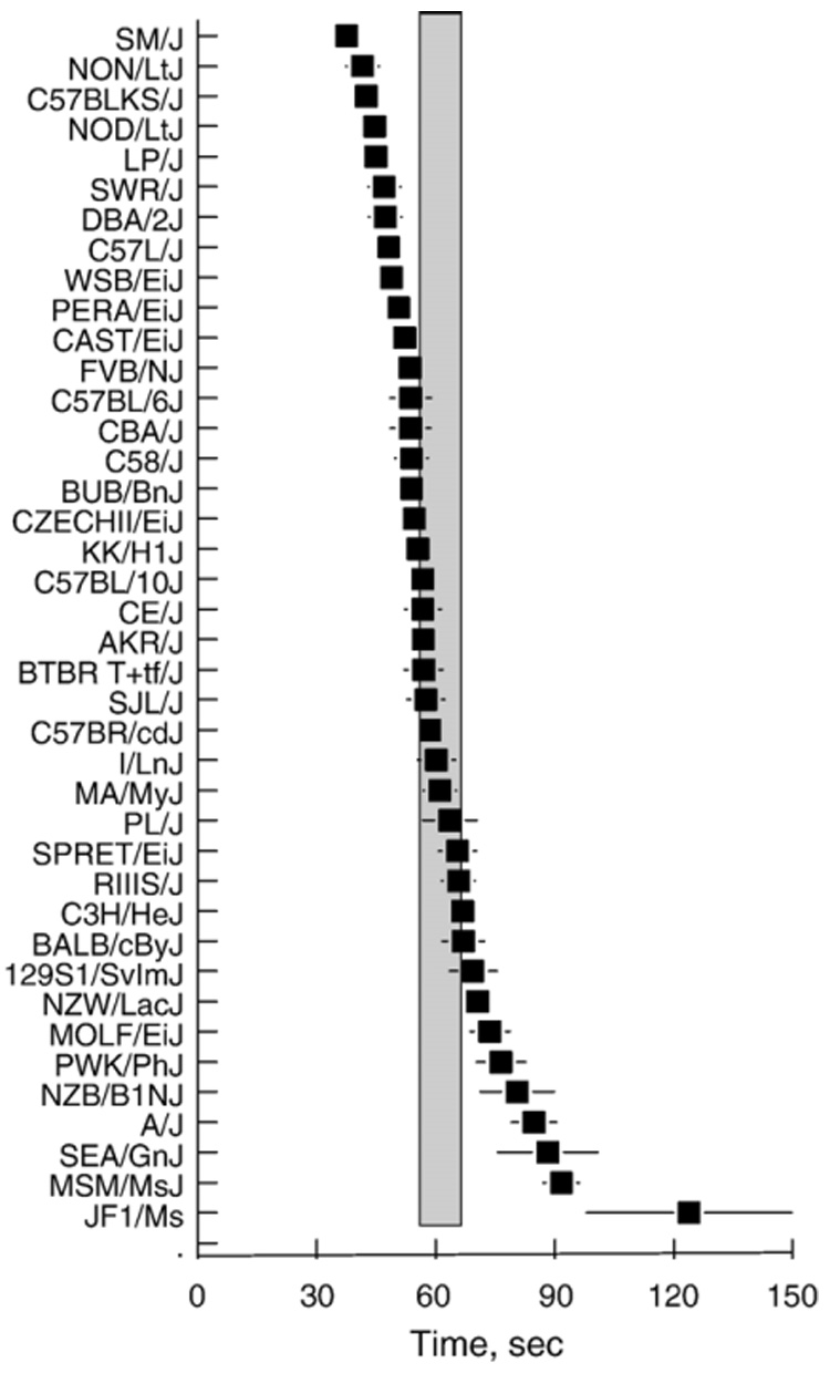
Time required to collect a 40-µl blood sample from the tail for 40 strains of mice. Strains are arranged in order from easiest to most difficult bleeders. Symbols represent average of males and females (~20 mice/strain). Vertical shaded bar shows 95% confidence intervals from the overall mean. Horizontal lines are standard errors of the mean; these are smaller than the symbols in most cases.

There were strain differences in blood pH (Fig. 5), and pH had a noticeable effect on adjusted blood ionized calcium levels in some strains (Fig. 6). Not surprisingly, pH was strongly related to pH-adjusted ionized calcium (r=0.70, n=40) but was independent of unadjusted ionized calcium (r=0.07, n=40). There was an inverse relationship between pH and plasma total calcium (r=−0.27, n=40).

Fig. 5.

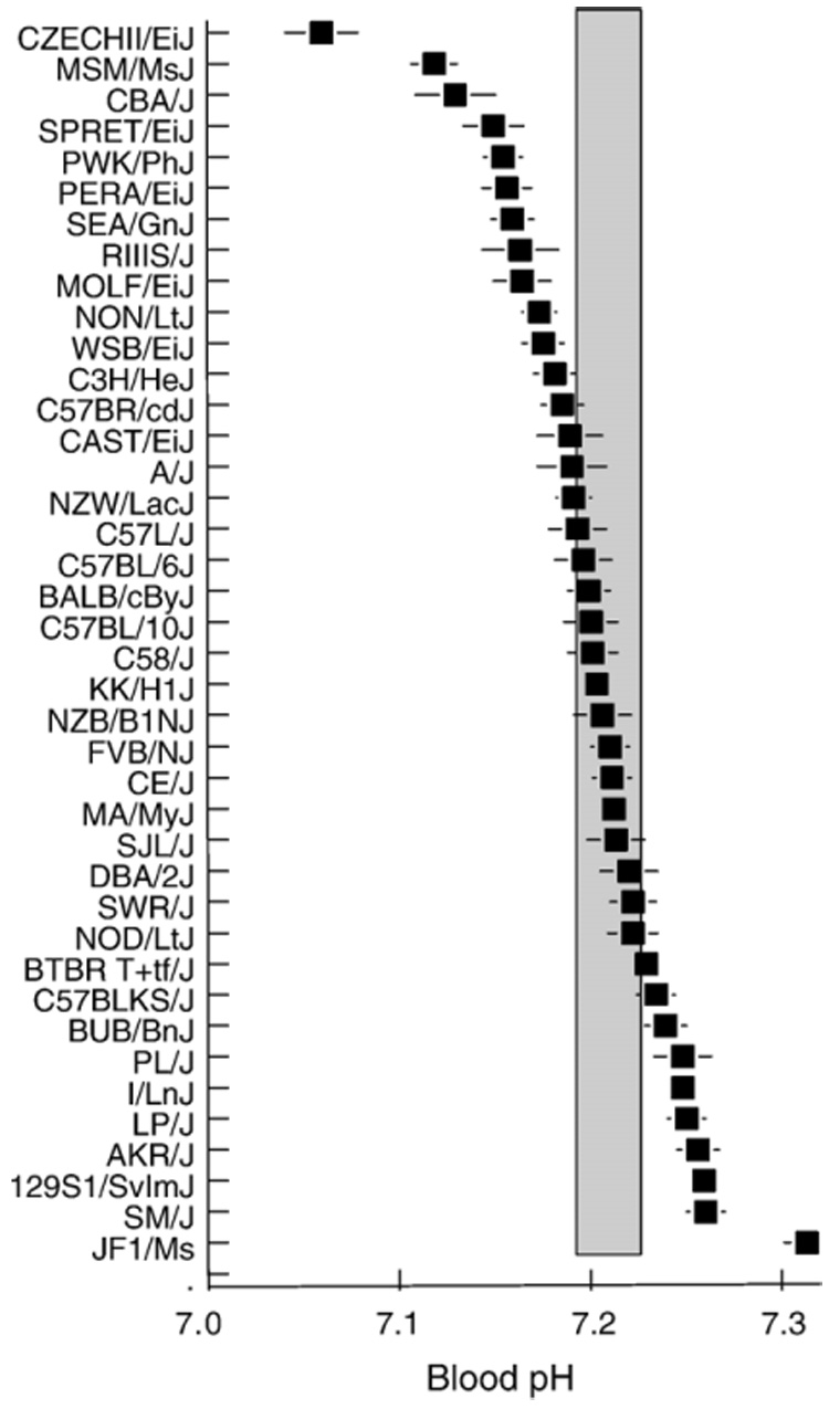
Blood pH of 40 strains of mice. Strains are arranged in order from lowest to highest pH. Symbols represent average of males and females (~20 mice/strain). Vertical shaded bar shows 95% confidence intervals from the overall mean. Horizontal lines are standard errors of the mean.

Fig. 6.

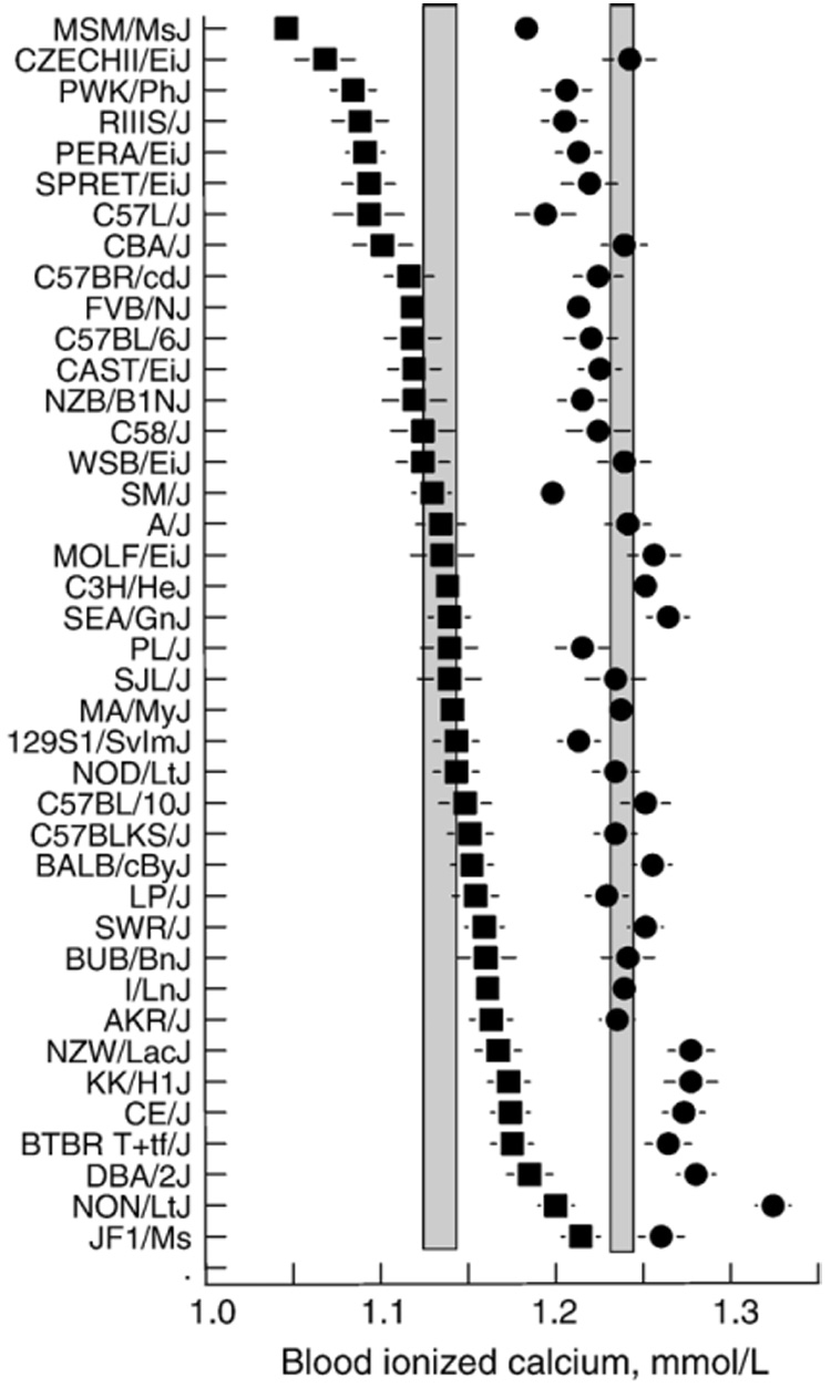
Blood ionized calcium concentrations of mice from 40 strains. Symbols represent average of males and females (~20 mice/strain). Circles=blood ionized calcium without adjustment for pH. Squares=blood ionized calcium adjusted for pH. Vertical shaded bars show 95% confidence intervals from the overall mean. Horizontal lines are standard errors of the mean.

Plasma total calcium concentrations of the 40 strains (Fig. 7) had a moderate correlation with blood ionized calcium concentrations (r=0.40, n=40), and a much weaker correlation with adjusted blood ionized calcium concentrations (r=0.11).

Fig. 7.

Plasma total calcium concentrations of mice from 40 strains. Strains are arranged in order from lowest to highest plasma total calcium. Symbols represent average of males and females (~20 mice/strain). Vertical shaded bar shows 95% confidence intervals from the overall mean. Horizontal lines are standard errors of the mean.

There were no significant correlations between any of the blood measures and calcium intake (Table 3).

Table 3.

Correlations of adjusted calcium intakes with measures of blood and bone calcium

	Solution ingested
	CaCl2			CaLa
Physiological measure	7.5 mM	25 mM	75 mM	7.5 mM	25 mM	75 mM
Blood pH	−0.01	−0.09	0.06	−0.07	−0.06	0.04
Blood Cai	−0.02	−0.01	−0.11	−0.08	−0.06	−0.04
Blood Cai adj. pH	−0.02	−0.06	−0.03	−0.10	−0.08	−0.00
Plasma total calcium	−0.09	−0.22	−0.29	−0.13	−0.26	−0.33
Bone mineral density	−0.12	−0.26	−0.19	−0.25	−0.24	−0.23
Bone mineral content	−0.09	−0.22	−0.16	−0.23	−0.19	−0.16

Correlation coefficients are based on the mean values for 40 strains (both sexes combined). None were significant. Blood Ca_i = blood ionized calcium; blood Ca_{i adj. pH} = blood ionized calcium adjusted for pH.

2.7. Bone mineral density and content

Over all strains combined, females had slightly but significantly denser bones [female=54.4±0.2 mg/cm², male=52.5±0.2 mg/cm²; F(1, 707)=46.1, p<0.00001] and higher BMC [female=454±3 mg; male=435±3 mg; F(1, 707)=20.0, p<0.00001]. Although the interaction of strain × sex was significant for both BMD and BMC, very few strains had significant sex differences (BMD; C57BR/cdJ, C57L/J and KK/H1J; F(39, 707)=3.41, p<0.00001; BMC; C57BR/cdJ, NON/LtJ and PERA/EiJ; F(39,707)=3.91, p<0.00001).

Given that most strains did not show sex differences, data from both sexes combined were used in subsequent analyses and for display (Fig. 8). For the 40 strains, the correlation between BMD and BMC was r=0.89; the correlation between BMD and carcass body weight was r=0.33, and between BMC and carcass body weight was r=0.29. Correlations of bone measures with calcium intake were all negative but nonsignificant (Table 3).

Fig. 8.

Bone mineral density (BMD; squares) and bone mineral content (BMC; circles) of mice from 40 strains. Strains are arranged in order from lowest to highest BMD. Symbols represent average of males and females (~20 mice/strain). The only strains with sex differences were C57BR/cdJ, C57L/J and KK/H1J for BMD, and C57BRcd/J, NON/LtJ and PERA/EiJ for BMC. Vertical shaded bars show 95% confidence intervals from the overall mean. Horizontal lines are standard errors of the mean; these are smaller than the symbols in most cases.

2.8. Heritability

Heritability was calculated from the ratio of SS_{among strains}/SS_total where SS is the sum of squares obtained in a one-way ANOVA based on data from each sex of each strain, or both sexes of each strain [8]. Heritability coefficients of calcium intake ranged from 0.41–0.72, depending on the particular sex, concentration and anion being tested (Table 4). In most cases, calcium preference scores had slightly higher heritability coefficients than did calcium intakes. Heritability of measures related to blood calcium was low (range 0.19–0.32) whereas BMD and BMC were moderately strongly heritable (range 0.66–0.77).

Table 4.

Estimates of heritability for some of the measures collected in this study

Measure	Both sexes	Males only	Females only
7.5 mM CaCl2 intake	0.70	0.54	0.68
25 mM CaCl2 intake	0.55	0.46	0.54
75 mM CaCl2 intake	0.53	0.41	0.53
7.5 mM CaLa intake	0.72	0.71	0.51
25 mM CaLa intake	0.63	0.56	0.51
75 mM CaLa intake	0.64	0.66	0.46
Sample collection time	0.26	0.27	0.31
Blood ionized Ca	0.19	0.30	0.22
Blood pH	0.39	0.46	0.41
Blood adjusted ionized calcium	0.25	0.32	0.29
Plasma total calcium	0.21	0.23	0.27
Bone mineral density	0.68	0.76	0.72
Bone mineral content	0.66	0.67	0.77

Heritability estimates are based on the ratio of SS_{among strains}/SS_total.

3. Discussion

The results illustrate the wide range of calcium intakes among mouse strains. There was a more-or-less continuous distribution of calcium intakes, which depended to some extent on the anion and concentration of calcium being considered. However, four strains, the PWK/PhJ, BTBR T⁺tf/J, JF1/Ms, and MA/MyJ, had noticeably higher intakes and preferences of both calcium anions at most concentrations than did the rest. These strains “liked” calcium in the sense that they preferred to drink it rather than water (Table 2). In contrast, several strains including the KK/H1J, C57BL/10J, CE/J and C58/J had consistently low calcium intakes and avoided even the lowest concentration relative to water. There was a 5-fold difference between the strains with the lowest and highest calcium intakes overall (C57BL/10J, 9.2 mL/kg^0.667/d; PWK/PhJ, 48.8 mL/kg^0.006/d).

The range of calcium intakes found here is much greater than that observed in a study of male mice from 28 strains that were tested with 3, 10, 30 and 100 mM CaCl₂ [1]. This appears to be due to the greater range of strains tested rather than procedural differences. The results from male mice of the 24 strains common to both studies correspond relatively strongly [r=0.72 between intakes of similar CaCl₂ concentrations (30 mM vs. 25 mM CaCl₂)], particularly given that the mice were different ages and were fed diets differing markedly in calcium content [130 mmol/kg here vs. ~250 mmol/kg in Ref. [1]]. The 16 strains unique to this study included several with much higher calcium intakes than any of the 28 strains tested earlier. The C3H/HeJ strain had the highest 30 mM CaCl₂ preference in the earlier study but was ranked 18th from highest intake of 25 mM CaCl₂ here. The “extra” strains tested here tended to be less commonly used and genealogically more diverse than those chosen for the 28-strain study. In summary, comparison of the two studies shows that the relative rankings of calcium intake across strains is robust, and that there is considerable benefit to be gained from testing a larger, or at least more genetically diverse, set of strains than the 28 used in earlier work. This is a sobering conclusion given that most strain surveys of other phenotypes are considerably smaller and tend to concentrate on common laboratory strains. Such studies do not encompass the genetic and phenotypic diversity that can be obtained by including less common and wild-derived strains.

3.1. Influence of concentration and anion on calcium intake

One of the most consistent findings of this study was that the higher the concentration of calcium given to drink, the lower the volume intake. There were modest-to-strong correlations between strain mean intakes of CaCl₂ and the corresponding concentrations of CaLa (Table 1, Fig. 1). Only one strain, the JF1/Ms, drank more CaCl₂ than CaLa; most drank more CaLa than CaCl₂. This higher preference for lactate than chloride is consistent with data from rats [21,52] and stands in contrast to the results found when the mice used here were tested with NaCl and NaLa [62]. Human psychophysical and rat gustatory electrophysiological studies show that the intensity of saltiness is inversely related to anion size [20,36,37], so it is likely that mice perceive lactate compounds as less intense than the chloride compounds. One possibility that fits the general pattern of the results is that mice drink more CaLa than CaCl₂ to reduce exposure to the “bad” taste of calcium but drink more NaCl than NaLa to increase exposure to the “good” taste of sodium.

Because the mice used in this paper to assess CaCl₂ and CaLa preferences were also used to assess NaCl and NaLa preferences [see [62]] it was possible to examine the contribution of cations and anions to the response to each taste solution. Relative to correlations within the calcium or sodium cations [average of 36 correlations for calcium, r=0.78, (Table 1) and for sodium, r=0.76 [62]] correlations between calcium and sodium solutions were low (average of 36 correlations, r=0.25, range 0.09–0.45; see [57] for individual correlations). Moreover, correlations between solutions with the same anion (e.g., 75 mM NaLa and 75 mM CaLa; average correlation, r=0.27) were no greater than those between solutions with the alternate anion (e.g,. 75 mM NaCl and 75 mM CaLa; average correlation, r=0.23). Thus, the contribution of the cation was considerably more important in determining preference than the contribution of the anion.

All mice were tested with an ascending series of three CaCl₂ solutions and then an ascending series of three CaLa solutions. We chose not to use a counterbalanced test order because our main goal was to characterize genetic effects and the additional variance introduced would have diluted these. The down-side of this is that we do not know whether the response to solutions presented early in the experiment influenced later ones. We are unaware of any demonstrations of carry-over effects with calcium solutions, although they are clearly a factor in tests involving NaCl [e.g. [3,4]]. We thus caution that the responses to CaLa may have been influenced by prior experience with CaCl₂ and that CaLa preferences may differ in naïve mice.

3.2. Sex differences in calcium consumption

Several studies show that female rats have a greater avidity for calcium than do males [41,42,44] and that female reproductive steroids increase calcium consumption [16,28,41]. This may not be a universal phenomenon, however. In the present study, females from only 13 of the 40 strains drank significantly more of at least one concentration of calcium than did same-strain males. Even this may exaggerate the frequency of sex differences, because the lighter weight of females biases adjusted fluid intakes upwards relative to unadjusted intakes. There were sex differences in unadjusted intakes in only 8 strains, and sex differences in calcium preference scores in only 5 strains.

It is generally believed that females have higher calcium intakes than males because of the demands of pregnancy and lactation [16,28,41]. However, we could find no obvious relationship between calcium intake measured here and reports of the ease of breeding, typical litter size or other measures of reproductive success [see [22]]. Given that more than two-thirds of the strains did not differ by sex in calcium consumption, the reason why some strains show sex differences may have to be reconsidered.

3.3. Blood calcium

The only previous strain survey of blood calcium levels was limited to measurement of serum total calcium from male mice of 5 strains [5]. The present study was much more comprehensive. We took measurements of both ionized and total calcium from 40 strains of mice of both sexes.

Calcium circulates in the blood in equilibrium between the ionized or “free” form, and “bound” form, attached to complexes and proteins. The ionized form is biologically active, and so arguably of most interest, but it is difficult to measure. Ionized calcium is pH-sensitive and during sample processing, blood pH increases due to the loss of dissolved CO₂. To account for this, measured ionized calcium concentrations are routinely adjusted according to a standard formula [11]. This practice, while appropriate in the clinic, would obscure intrinsic differences in blood pH between strains. Consequently, to avoid the need for it, we tried to reduce sampling and processing times as much as was practical by analyzing whole blood (rather than plasma, to reduce processing time) and housing the calcium analyzer in the vivarium (reducing sample transfer time). We were also concerned that it would take longer to restrain and bleed some of the wilder mice than their more domesticated cousins but this proved to be untrue (Fig. 4). Blood coagulation appeared to be a much more critical factor in determining the time needed to collect samples. We note that rapid coagulation made obtaining blood from the JF1/Ms strain noticeably more difficult than from any other strain even though this was one of the most docile strains we tested. As far as we are aware, this hematological anomaly of the JF1/Ms strain has not been reported previously.

We suspect the outlying blood pH of the JF1/Ms strain (see Fig. 5) was at least in part due to the difficulty of sampling its blood (see Fig. 4). For the remaining strains, the interval between blood sampling and analysis was relatively consistent, and there was no relationship between sampling time and pH (r=0.02). This implies that the blood pH values we measured most likely reflect physiological differences among strains rather than sample processing times, and it is thus inappropriate to correct blood ionized calcium for pH. Consistent with this, strain mean total calcium concentrations were more strongly related to unadjusted than pH-adjusted ionized calcium concentrations (r=0.40 vs. r=0.11).We note that adjustment for pH can make a considerable difference to strain rankings. For example, the CZECHII/EiJ strain was ranked 39th in unadjusted but 14th in pH-adjusted blood calcium levels (Fig. 6).

None of the measures of blood calcium was significantly related to any of the measures of calcium intake, although all the correlations were negative (Table 3). This does not strongly support the hypothesis that a signal related to low blood calcium controls calcium intake (see Ref. [54]), although the direction of the correlation is consistent with such a relationship. If the hypothesis is correct, a weak negative correlation might be expected for at least two reasons: first, blood was collected in the middle of the light period, when mice were unlikely to ingest calcium, so physiology and behavior were temporally distinct. Second, recent intake of calcium in food or solution may have influenced blood calcium levels. This may also be responsible for the low coefficients of heritability observed with blood-related measures.

3.4. Bone mineral density and content

Bone mineral content and morphology are among the most common phenotypes used in QTL analyses, but these have been confined to just a few strains [primarily AKR/J, C57BL/6J, CAST/EiJ, DBA/2, MRL/MpJ, SJL/J and SAMP [6,7,9,15,17,18,26,27,29,31,38,46–48]. The present results provide a basis for extending these studies to other strains, including some with more extreme phenotypes than those used previously.

Consistent with many QTL studies, bone mineral density and content were highly heritable. There was no significant relationship between bone mineral density or content and calcium intake. This suggests that if a feedback signal from bone exists its effects on calcium intake are subtle. We saw no effect of calcium solution consumption on bone mineral content but this is not surprising given the relatively small contribution of calcium solution intake to total calcium intake: over the 12 days of tests, each mouse consumed ~15 mg Ca²⁺ from calcium solutions but >300 mg Ca²⁺ from food.

3.5. Calcium consumption compared with other phenotypes

The results obtained here and in accompanying papers suggest that there is no simple relationship between calcium consumption and blood calcium concentrations, bone calcium, water intake, sodium intake, or body composition [40,62]. Comparisons of the results found here with data in the Mouse Phenome Database [49] suggest that consumption of at least one concentration of calcium is positively related to red blood cell hemoglobin concentrations, the percentage of leukocytes that are neutrophils, white blood cell count, various measures of heart weight, and taste preferences for 30 and 300 mM NH₄Cl. Calcium consumption is also inversely related to blood leukocyte count, various measures of activity (beam crosses), daily food intake, and corpus callosum and hippocampal commisure morphology. Such correlations may suggest physiological mechanisms participating in the control of calcium intake, although of course, many may also be epiphenomena.

3.6. Different mechanisms underlie the avidity for calcium in different strains

We have paid particular attention to identifying commonalities among the PWK/PhJ, BTBR T⁺tf/J, JF1/Ms and MA/MyJ strains because each had notably higher calcium intakes and preferences than did the other 36 strains tested. One of these strains, the MA/MyJ strain, has been reported to be polydipsic [10]. In our hands, it had relatively normal intakes of water [62] but very high intakes of both calcium and sodium [62]. This nonspecific proclivity to drink fluids reduces enthusiasm for using the MA/MyJ strain to identify genes underlying calcium consumption. We note that the other three avid calcium-consuming strains were not polydipsic, and not all polydipsic strains have high calcium solution intakes. Indeed, the strain with the second highest water intakes in this study (C58/J) had among the lowest calcium intakes.

Of the remaining three avid calcium-consuming strains, there does not appear to be a common factor that can account for their higher intakes. Perhaps this is not surprising given their genetic diversity. The origins of the BTBR T⁺tf/J strain are obscure but SNP parsimony analysis suggests it is similar to some of the 129 strains and thus most likely derived from Mus musculus domesticus stock owned by Castle [39]. The PWK/PhJ strain is derived from Mus musculus musculus and the JF1/Ms strain is derived from Mus musculus molossinus. It would be difficult to envision a more diverse trio of laboratory mouse strains. This diversity implies that the genetic architecture underlying calcium intake in these strains is more likely to differ than if the strains were closely related.

We note that the three avid calcium-drinking strains were frequently ranked at opposite extremes of the distributions of the physiological measures we collected. Whereas the JF1/Ms strain had the highest ionized calcium intakes of any strain, the PWK/PhJ strain was ranked 38th out of 40. The BTBR T⁺tf/J strain had the highest bone mineral content of the 40 strains tested, whereas the JF1/Ms strain had the lowest bone mineral content. The presence of avid calcium-drinking strains at the distribution extremes suggests there may be a connection between “extreme” physiology and “extreme” behavior, but this is obscured because different genetic mechanisms are at play in different strains. We anticipate that ongoing genetic and physiological analyses of these outlying strains will reveal the mechanisms responsible for the variation in calcium consumption.

References

- 1.Bachmanov AA, Beauchamp GK, Tordoff MG. Avidity for KCl, NH4Cl, CaCl2 and NaCl solutions by 28 mouse strains. Behav Genet. 2002;32:445–457. doi: 10.1023/a:1020832327983. [DOI] [PMC free article] [PubMed] [Google Scholar]
- 2.Bachmanov AA, Reed DR, Beauchamp GK, Tordoff MG. Body weight, food intake, water intake, and drinking spout side preference of 28 mouse strains. Behav Genet. 2002;32:435–443. doi: 10.1023/a:1020884312053. [DOI] [PMC free article] [PubMed] [Google Scholar]
- 3.Bachmanov AA, Schlager G, Tordoff MG, Beauchamp GK. Consumption of electrolytes and quinine by mouse strains with different blood pressures. Physiol Behav. 1998;64:323–330. doi: 10.1016/s0031-9384(98)00069-9. [DOI] [PMC free article] [PubMed] [Google Scholar]
- 4.Bachmanov AA, Tordoff MG, Beauchamp GK. Voluntary sodium chloride consumption by mice: differences among five inbred strains. Behav Genet. 1998;28:117–124. doi: 10.1023/a:1021471924143. [DOI] [PMC free article] [PubMed] [Google Scholar]
- 5.Barrett CP, Donati EJ, Volz JE, Smith EB. Variations in serum calcium between strains of inbred mice. Lab Anim Sci. 1975;25:638–640. [PubMed] [Google Scholar]
- 6.Beamer WG, Shultz KL, Churchill GA, Frankel WN, Baylink DJ, Rosen CJ, et al. Quantitative trait loci for bone density in C57BL/6J and CAST/EiJ inbred mice. Mamm Genome. 1999;10:1043–1049. doi: 10.1007/s003359901159. [DOI] [PubMed] [Google Scholar]
- 7.Beamer WG, Shultz KL, Donahue LR, Churchill GA, Sen S, Wergedal JR, et al. Quantitative trait loci for femoral and lumbar vertebral bone mineral density in C57BL/6J and C3H/HeJ inbred strains of mice. J Bone Miner Res. 2001;16:1195–1206. doi: 10.1359/jbmr.2001.16.7.1195. [DOI] [PubMed] [Google Scholar]
- 8.Belknap JK. Effect of within-strain sample size on QTL detection and mapping using recombinant inbred mouse strains. Behav Genet. 1998;28:29–38. doi: 10.1023/a:1021404714631. [DOI] [PubMed] [Google Scholar]
- 9.Benes H, Weinstein RS, Zheng W, Thaden JJ, Jilka RL, Manolagas SC, et al. Chromosomal mapping of osteopenia-associated quantitative trait loci using closely related mouse strains. J Bone Miner Res. 2000;15:626–633. doi: 10.1359/jbmr.2000.15.4.626. [DOI] [PubMed] [Google Scholar]
- 10.Bernstein SE. Physiological characteristics. In: Green EL, editor. Biology of the Laboratory Mouse. 2nd ed. New York: McGraw-Hill; 1966. pp. 337–350. [Google Scholar]
- 11.Boink ABTJ, Buckley BM, Christiansen TF, Covington AK, Maas AHJ, Muller-Plathe O, et al. IFCC recommendation on sampling, transport and storage for the determination of the concentration of ionized calcium in whole blood, plasma and serum. J Automat Chem. 1991;13:235–239. doi: 10.1155/S1463924691000391. [DOI] [PMC free article] [PubMed] [Google Scholar]
- 12.Brommage R, DeLuca HF. Self-selection of a high calcium diet by vitamin D-deficient lactating rats increases food consumption and milk production. J Nutr. 1984;114:1377–1385. doi: 10.1093/jn/114.8.1377. [DOI] [PubMed] [Google Scholar]
- 13.Coldwell SE, Tordoff MG. Latent learning about calcium and sodium. Am J Physiol. 1993;265:R1480–R1484. doi: 10.1152/ajpregu.1993.265.6.R1480. [DOI] [PubMed] [Google Scholar]
- 14.Coldwell SE, Tordoff MG. Immediate acceptance of minerals and HCl by calcium-deprived rats: brief exposure tests. Am J Physiol. 1996;271:R11–R17. doi: 10.1152/ajpregu.1996.271.1.R11. [DOI] [PubMed] [Google Scholar]
- 15.Corva PM, Horvat S, Medrano JF. Quantitative trait loci affecting growth in high growth (hg) mice. Mamm Genome. 2001;12:284–290. doi: 10.1007/s003350010275. [DOI] [PubMed] [Google Scholar]
- 16.Denton DA, Nelson JF. Effects of pregnancy and lactation on the mineral appetites of wild rabbits [Oryctolagus cuniculus (L.)] Endocrinology. 1971;88:31–40. doi: 10.1210/endo-88-1-31. [DOI] [PubMed] [Google Scholar]
- 17.Drake TA, Hannani K, Kabo JM, Villa V, Krass K, Lusis AJ. Genetic loci influencing natural variations in femoral bone morphometry in mice. J Orthop Res. 2001;19:511–517. doi: 10.1016/S0736-0266(00)00056-5. [DOI] [PubMed] [Google Scholar]
- 18.Drake TA, Schadt E, Hannani K, Kabo JM, Krass K, Colinayo V, et al. Genetic loci determining bone density in mice with diet-induced atherosclerosis. Physiol Genomics. 2001;5:205–215. doi: 10.1152/physiolgenomics.2001.5.4.205. [DOI] [PubMed] [Google Scholar]
- 19.Dyets Inc. 100000 AIN-76A Purified rodent diet. 2003 http://www.dyets.com/100000.htm.
- 20.Dzendolet E, Meiselman HL. Cation and anion contributions to gustatory quality of simple salts. Percept Psychophys. 1967;2:601–604. [Google Scholar]
- 21.Ferrell F, Dreith AZ. Calcium appetite, blood pressure and electrolytes in spontaneously hypertensive rats. Physiol Behav. 1986;37:337–343. doi: 10.1016/0031-9384(86)90243-x. [DOI] [PubMed] [Google Scholar]
- 22.Festing MFW. Inbred strains of mice. The Jackson Laboratory. 1998 http://www.informatics.jax.org/external/festing/mouse/INTRO.shtml.
- 23.Hughes BO, Wood-Gush DGM. A specific appetite for calcium in domestic chicken. Anim Behav. 1971;19:490–499. doi: 10.1016/s0003-3472(71)80103-3. [DOI] [PubMed] [Google Scholar]
- 24.Hughes BO, Wood-Gush DGM. Hypothetical mechanisms underlying calcium appetite in fowls. Rev Comport Anim. 1972;6:95–106. [Google Scholar]
- 25.Inoue M, Tordoff MG. Calcium deficiency alters chorda tympani nerve responses to oral calcium chloride. Physiol Behav. 1998;63:297–303. doi: 10.1016/s0031-9384(97)00387-9. [DOI] [PubMed] [Google Scholar]
- 26.Klein RF, Mitchell SR, Phillips TJ, Belknap JK, Orwoll ES. Quantitative trait loci affecting peak bone mineral density in mice. J Bone Miner Res. 1998;13:1648–1656. doi: 10.1359/jbmr.1998.13.11.1648. [DOI] [PubMed] [Google Scholar]
- 27.Klein RF, Turner RJ, Skinner LD, Vartanian KA, Serang M, Carlos AS, et al. Mapping quantitative trait loci that influence femoral cross-sectional area in mice. J Bone Miner Res. 2002;17:1752–1760. doi: 10.1359/jbmr.2002.17.10.1752. [DOI] [PubMed] [Google Scholar]
- 28.Leshem M, Levin T, Schulkin J. Intake and hedonics of calcium and sodium during pregnancy and lactation in the rat. Physiol Behav. 2002;75:313–322. doi: 10.1016/s0031-9384(01)00668-0. [DOI] [PubMed] [Google Scholar]
- 29.Li X, Masinde G, Gu W, Wergedal J, Mohan S, Baylink DJ. Genetic dissection of femur breaking strength in a large population (MRL/MpJ x SJL/J) of F2 Mice: single QTL effects, epistasis, and pleiotropy. Genomics. 2002;79:734–740. doi: 10.1006/geno.2002.6760. [DOI] [PubMed] [Google Scholar]
- 30.Lobaugh B, Joshua IG, Mueller WJ. Regulation of calcium appetite in broiler chickens. J Nutr. 1981;111:298–306. doi: 10.1093/jn/111.2.298. [DOI] [PubMed] [Google Scholar]
- 31.Masinde GL, Li X, Gu W, Wergedal J, Mohan S, Baylink DJ. Quantitative trait loci for bone density in mice: the genes determining total skeletal density and femur density show little overlap in F2 mice. Calcif Tissue Int. 2002;71:421–428. doi: 10.1007/s00223-001-1113-z. [DOI] [PubMed] [Google Scholar]
- 32.McCaughey SA, Fitts DA, Tordoff MG. Lesions of the subfornical organ decrease the calcium appetite of calcium-deprived rats. Physiol Behav. 2003;79:605–612. doi: 10.1016/s0031-9384(03)00139-2. [DOI] [PubMed] [Google Scholar]
- 33.McCaughey SA, Forestell CA, Tordoff MG. Calcium deprivation increases the palatability of calcium solution in rats. Physiol Behav. 2005;84:335–342. doi: 10.1016/j.physbeh.2004.12.010. [DOI] [PubMed] [Google Scholar]
- 34.McCaughey SA, Tordoff MG. Calcium-deprived rats sham-drink CaCl2 and NaCl. Appetite. 2000;34:305–311. doi: 10.1006/appe.1999.0317. [DOI] [PubMed] [Google Scholar]
- 35.McCaughey SA, Tordoff MG. Calcium deprivation alters gustatory-evoked activity in the rat nucleus of the solitary tract. Am J Physiol Regul Integr Comp Physiol. 2001;281:R971–R978. doi: 10.1152/ajpregu.2001.281.3.R971. [DOI] [PubMed] [Google Scholar]
- 36.Murphy C, Cardello AV, Brand JG. Tastes of fifteen halide salts following water and NaCl: anion and cation effects. Physiol Behav. 1981;26:1083–1095. doi: 10.1016/0031-9384(81)90213-4. [DOI] [PubMed] [Google Scholar]
- 37.Nakamura M, Kurihara K. Rat taste nerve responses to salts carrying cations of large molecular size; are the taste responses to the salts induced by cation transport across apical membranes of taste cells? Comp Biochem Physiol. 1991;100A:661–665. doi: 10.1016/0300-9629(91)90386-q. [DOI] [PubMed] [Google Scholar]
- 38.Orwoll ES, Belknap JK, Klein RF. Gender specificity in the genetic determinants of peak bone mass. J Bone Miner Res. 2001;16:1962–1971. doi: 10.1359/jbmr.2001.16.11.1962. [DOI] [PubMed] [Google Scholar]
- 39.Petkov PM, Ding Y, Cassell MA, Zhang W, Wagner G, Sargent EE, et al. An efficient SNP system for mouse genome scanning and elucidating strain relationships. Genome Res. 2004;14:1806–1811. doi: 10.1101/gr.2825804. [DOI] [PMC free article] [PubMed] [Google Scholar]
- 40.Reed DR, Bachmanov AA, Tordoff MG. Forty mouse strain survey of body weight and composition. Physiol Behav. doi: 10.1016/j.physbeh.2007.03.026. in press, doi:10.1016/j.physbeh.2007.03.026. [DOI] [PMC free article] [PubMed]
- 41.Reilly JJ, Epstein AN, Schulki J. Hormonal control of calcium ingestion: the effects of neonatal gonadectomy on the calcium ingestion of male and female rats. SSIB. 1992;53 [Google Scholar]
- 42.Reilly JJ, Nardozzi J, Schulkin J. The ingestion of calcium in multiparous and virgin female rats. Brain Res Bull. 1995;37:301–303. doi: 10.1016/0361-9230(95)00036-e. [DOI] [PubMed] [Google Scholar]
- 43.Richter CP, Eckert JF. Increased calcium appetite of parathyroidectomized rats. Endocrinology. 1937;21:50–54. [Google Scholar]
- 44.Schulkin J. The ingestion of calcium in female and male rats. Psychobiology. 1991;19:262–264. [Google Scholar]
- 45.Schulkin J. Calcium hunger. Cambridge: Cambridge University Press; 2001. [Google Scholar]
- 46.Shimizu M, Higuchi K, Bennett B, Xia C, Tsuboyama T, Kasai S, et al. Identification of peak bone mass QTL in a spontaneously osteoporotic mouse strain. Mamm Genome. 1999;10:81–87. doi: 10.1007/s003359900949. [DOI] [PubMed] [Google Scholar]
- 47.Shimizu M, Higuchi K, Kasai S, Tsuboyama T, Matsushita M, Mori M, et al. Chromosome 13 locus, Pbd2, regulates bone density in mice. J Bone Miner Res. 2001;16:1972–1982. doi: 10.1359/jbmr.2001.16.11.1972. [DOI] [PubMed] [Google Scholar]
- 48.Shultz KL, Donahue LR, Bouxsein ML, Baylink DJ, Rosen CJ, Beamer WG. Congenic strains of mice for verification and genetic decomposition of quantitative trait loci for femoral bone mineral density. J Bone Miner Res. 2003;18:175–185. doi: 10.1359/jbmr.2003.18.2.175. [DOI] [PubMed] [Google Scholar]
- 49.The Jackson Laboratory. Mouse phenome database web site. 2001 http://www.jax.org/phenome.
- 50.The Jackson Laboratory. Recommended inbred strains. 2001 http://aretha.jax.org/pub-cgi/phenome/mpdcgi?rtn=docs/recommendations#strains.
- 51.Tordoff MG, Hughes R, Pilchak D. Calcium intake by the rat: influence of parathyroid hormone, calcitonin, and 1,25-dihydroxyvitamin D. Am J Physiol. 1998;274:R214–R231. doi: 10.1152/ajpregu.1998.274.1.R214. [DOI] [PubMed] [Google Scholar]
- 52.Tordoff MG. Influence of dietary calcium on sodium and calcium intake of spontaneously hypertensive rats. Am J Physiol. 1992;262:R370–R381. doi: 10.1152/ajpregu.1992.262.3.R370. [DOI] [PubMed] [Google Scholar]
- 53.Tordoff MG. Voluntary intake of calcium and other minerals by rats. Am J Physiol. 1994;267:R470–R475. doi: 10.1152/ajpregu.1994.267.2.R470. [DOI] [PubMed] [Google Scholar]
- 54.Tordoff MG. Calcium: taste, intake and appetite. Physiol Rev. 2001;81:1567–1597. doi: 10.1152/physrev.2001.81.4.1567. [DOI] [PubMed] [Google Scholar]
- 55.Tordoff MG. Intragastric calcium infusions support flavor preference learning by calcium-deprived rats. Physiol Behav. 2002;76:521–529. doi: 10.1016/s0031-9384(02)00723-0. [DOI] [PubMed] [Google Scholar]
- 56.Tordoff MG, Bachmanov AA. Monell mouse taste phenotyping project. Monell Chemical Senses Center. 2001 www.monell.org/MMTPP.
- 57.Tordoff MG, Bachmanov AA. Survey of calcium and sodium intake and metabolism with bone and body composition data (MPD:103) Mouse Phenome Project. 2002 http://phenome.jax.org/pub-cgi/phenome/mpdcgi?rtn=projects/details&id=103.
- 58.Tordoff MG, Bachmanov AA. Influence of the number of alcohol and water bottles on murine alcohol intake. Alcohol Clin Exp Res. 2003;27:600–606. doi: 10.1097/01.ALC.0000060529.30157.38. [DOI] [PMC free article] [PubMed] [Google Scholar]
- 59.Tordoff MG, Bachmanov AA. Mouse taste preference tests: Influence of drinking spout position. 2003 doi: 10.1093/chemse/28.4.315. http://www.monell.org/MMTPP/Verification%20-%20Spout%20position.htm. [DOI] [PMC free article] [PubMed]
- 60.Tordoff MG, Bachmanov AA. Mouse taste preference tests: why only two bottles? Chem. Senses. 2003;28:315–324. doi: 10.1093/chemse/28.4.315. [DOI] [PMC free article] [PubMed] [Google Scholar]
- 61.Tordoff MG, Hughes RL, Pilchak DM. Independence of salt intake from the hormones regulating calcium homeostasis. Am J Physiol. 1993;264:R500–R512. doi: 10.1152/ajpregu.1993.264.3.R500. [DOI] [PubMed] [Google Scholar]
- 62.Tordoff MG, Reed DR, Bachmanov AA. Forty mouse strain survey of water and sodium intake. Physiol Behav. doi: 10.1016/j.physbeh.2007.03.025. in press, doi:10.1016/j.physbeh.2007.03.025. [DOI] [PMC free article] [PubMed]