Congruence of Imaging Estimators and Mechanical Measurements of Viscoelastic Properties of Soft Tissues

Abstract

Biomechanical properties of soft tissues are important for a wide range of medical applications, such as surgical simulation and planning and detection of lesions by elasticity imaging modalities. Currently, the data in the literature is limited and conflicting. Furthermore, to assess the biomechanical properties of living tissue in vivo, reliable imaging-based estimators must be developed and verified. For these reasons we developed and compared two independent quantitative methods – crawling wave estimator (CRE) and mechanical measurement (MM) for soft tissue characterization. The CRE method images shear wave interference patterns from which the shear wave velocity can be determined and hence the Young’s modulus can be obtained. The MM method provides the complex Young’s modulus of the soft tissue from which both elastic and viscous behavior can be extracted. This article presents the systematic comparison between these two techniques on the measurement of gelatin phantom, veal liver, thermal-treated veal liver, and human prostate. It was observed that the Young’s moduli of liver and prostate tissues slightly increase with frequency. The experimental results of the two methods are highly congruent, suggesting CRE and MM methods can be reliably used to investigate viscoelastic properties of other soft tissues, with CRE having the advantages of operating in nearly real time and in situ.

INTRODUCTION

The biomechanical properties of soft tissues are intrinsically related to their composition. It is well known that pathological processes typically alter the stiffness of soft tissues. Therefore, digital palpation, a qualitative clinical tool, has been used for centuries to diagnose the presence of localized tumors in accessible regions of the human body. Recently, thermal therapy techniques such as radio frequency ablation (RFA), microwave, laser, and high-intensity focused ultrasound (HIFU) have been utilized to create tissue necrotic coagulation for killing tumors. Those necrotic lesions appear stiffer than surrounding tissue as well. A better understanding of the mechanical properties of soft tissues, including cancerous, thermal treated, and normal tissues, is of particular importance for biomechanics and medical applications, such as biomechanical modeling, surgical simulation and planning, and imaging pathologies by elasticity estimators.

Although mechanical properties of structural materials have been studied and well characterized by various mechanical testing methods for decades, little is known for most biological soft tissues. Moreover, the mechanical properties of human soft tissues, such as Young’s modulus and shear modulus, vary widely. For these reasons, various techniques have been developed to image and characterize soft tissue viscoelasticity for diagnostic and/or therapeutic monitoring. In the past two decades, five major elasticity imaging modalities have been established to non-invasively image hard lesions in soft tissues based on their elasticity contrast. They are either ultrasound (US)-based approaches such as vibration sonoelastography (Krouskop et al. 1987; Lerner et al. 1988; Parker et al. 1990; Yamakoshi et al. 1990), compression elastography (Ophir et al. 1991), transient elastography (Catheline et al. 1999; Sandrin et al. 2002a; Sandrin et al. 2002b) and acoustic radiation force (ARF)-related imaging (Bercoff et al. 2004; Fatemi and Greenleaf 1998; Nightingale et al. 2001; Sarvazyan et al. 1998), or magnetic resonance (MR) imaging-based approaches such as static MR elastography (MRE) (Fowlkes et al. 1995; Plewes et al. 1995) and dynamic MRE (Bishop et al. 1998; Muthupillai et al. 1995). Some of those noninvasive techniques have also been applied to measure soft tissue mechanical parameters directly.

An early clinical evaluation of elasticity of human liver in various diffuse diseases was reported by Sanada et al. (2000) using sonoelastographic measurement. The principle of the study is the same as that of the shear wave estimation method developed by Yamakoshi et al. (1990). The propagation of low-frequency vibration (40 Hz) in the liver was observed with a conventional Doppler imaging system, and the velocities related to shear elasticity were measured by vibration phase images. However, bias can be induced during measurement by refraction and reflection of the propagating vibration waves at tissue boundaries, diffraction effects (Catheline et al. 1999) and liver displacements during an acquisition time of 90 seconds. More recently, one-dimensional (1-D) transient elastography (FibroScan®: Echosens, Paris, France) was established for the assessment of liver stiffness (Sandrin et al. 2003). Supersonic shear imaging (SSI), an ARF-based method, was developed to characterize breast tissue in vivo (Bercoff et al. 2004).

The potential of dynamic MRE clinical implementation has been proven in preliminary human studies in which the data of human prostate, breast, brain, muscle, and liver were presented (Bensamoun et al. 2006; Bishop et al. 1998; Kemper et al. 2004; Kruse et al. 2000; Papazoglou et al. 2006; Rouviere et al. 2006; Sinkus et al. 2005). In particular, Kruse et al. (2000) evaluated porcine livers with MRE at multiple shear wave frequencies and reported that the wave velocity and the shear stiffness increased with frequency. The shear stiffness measured with MRE was 3 kPa at 100 Hz. This technique provides high-resolution images, although its long acquisition time (about 20 minutes) and high cost are a consideration.

Independently, mechanical testing-based methods can characterize soft tissue properties, and thus be used as a comparison to elasticity imaging methods. In practice, the reliable data on soft tissue properties are limited in the literature, although this need is vast. Several groups (Dunn and Silver 1983; Hof 2003; Huang et al. 2005; Klein et al. 2005; Kuo et al. 2001; Lally et al. 2004; Provenzano et al. 2002; Silver et al. 2001; Suki et al. 1994; Wu et al. 2003) have reported findings on mechanical properties of some soft tissues, but most of their studies were focused on tendons, ligaments, cartilage, skin, muscles, lungs, or arteries, which, to some extent, have active force-generating mechanical properties. In contrast, just a few publications (Arbogast and Margulies 1998; Chen et al. 1996; Darvish and Crandall 2001; Krouskop et al. 1998; Liu and Bilston 2000; Nasseri et al. 2002; Phipps et al. 2005a, 2005b; Snedeker et al. 2005; Yang and Church 2006; Yeh et al. 2002) presented quantitative results on the viscoelastic behavior of tissues such as brain, breast, prostate, liver, or kidney.

Liu and Bilston (2000) studied the viscoelastic properties of bovine liver tissue with three testing methods: shear strain sweep oscillation, shear stress relaxation, and shear oscillation. In the oscillation experiments, they found the storage shear modulus in a range of 1–6 kPa and the loss shear modulus in a range of several hundred Pa for applied frequencies from 0.006 to 20 Hz. They also confirmed that liver tissue has fluid-like viscoelastic behavior by analyzing the relaxation response of liver. In this study, they developed a linear 5-element Maxwell model and fit the experimental data to the model. The choice of tissue model seems to vary with different groups. Besides the three basic linear viscoelastic models (the Maxwell model, the Voigt model, and the Kelvin model) described by Fung (1993), other linear, quasi-linear or nonlinear models were also applied to fit the mechanical testing data. In particular, Szabo and Wu (2000) derived a generalized 3-parameter Kelvin-Voigt (KV) model for viscoelastic materials from the power law relationship. Taylor et al. (2002) further investigated the Kelvin-Voigt fractional derivative (KVFD) model by fitting the liver relaxation data to this model. Dynamic testing was performed by Kiss et al. (2004) on canine liver tissue, and the data were fit to both the KVFD model and the KV model. The complex Young’s modulus of the normal liver tissue was measured from 4 to 9 kPa over a frequency range from 0.1 to 100 Hz. By comparing the curve fitting results of the two models, they concluded that the KVFD model had better agreement with the experimental data than the KV model.

Krouskop et al. (1998) investigated the mechanical properties of normal and diseased breast and prostate tissues with a uniaxial compression indentor at low frequencies (0.1, 1, and 4 Hz). Their results showed that cancerous specimens had measurable elevated moduli compared to normal tissues in the same gland. They reported benign prostatic hyperplasia had significantly lower values (36–41 kPa) than normal tissue; the normal anterior and posterior tissue had elastic modulus values of 55–71 kPa under 2% or 4% precompression while cancer had values of 96–241 kPa. In addition, they noted that the storage modulus accounted for more than 90% of the complex modulus for frequencies above 1 Hz.

The biomechanical properties obtained from imaging methods such as MRE and SSI, however, were not in agreement with the abovementioned mechanical testing results on either breast or prostate specimens. With respect to the Young’s modulus, the SSI method provided a mean value 3 kPa of the normal breast tissue and an elevated value of breast cancer about 9 kPa (Bercoff et al. 2004). MRE measurements indicated that the peripheral portion of the prostate was stiffer than the central portion. The mean Young’s modulus values were 9.9 kPa and 6.6 kPa, respectively (Kemper et al. 2004). Significant discrepancies were also found on the reported stiffness of kidney tissue (Erkamp et al. 1998; Kruse et al. 2000; Nasseri et al. 2002; Snedeker et al. 2005). The divergent reports of soft tissue properties are mainly caused by the different choices of testing techniques, tissue models, compression frequencies, temperature, sample variation, and other experimental factors. The assumption of a particular tissue model, for example, purely elastic vs. viscoelastic, can greatly influence the estimates of tissue properties.

The scarcity and inconsistency of published data on soft tissue properties motivated us to develop reliable quantitative measurements for various soft tissues, which should be independent and congruent with each other. Therefore, we propose the crawling wave estimator (CRE) for visualizing shear wave interference patterns in phantom and soft tissues. The crawling waves generated by a pair of external shear wave sources (Piezo Systems, Cambridge, MA, USA) interfere with each other, appearing as moving parallel stripes in sonoelastography images. An earlier paper (Wu et al. 2004) proved that the spacing between the parallel strips is half of the shear wave wavelength. With the measured shear wave wavelength and the known driving signal frequency, we are able to calculate the shear wave velocity, and thus the Young’s modulus of the material. Many soft tissues show both elastic and viscous behavior under biomechanical characterization (Fung 1993). Hence, the stiffness of the tissue has a frequency dependent response to mechanical vibrations, presented as frequency dependent shear velocity and viscoelastic modulus. Independently, using MM of tissue core samples, we fit the stress relaxation data into the KVFD model for measuring the viscoelastic properties of soft tissues and compare the results to those obtained from the CRE method. In this study, our significant effort focused on evaluating the accuracy of the two independent quantitative tissue characterization techniques. Therefore, the congruence of the two techniques was investigated on selected soft tissues such as veal liver, thermal-treated veal liver, and human prostate tissue. In the literature, Chen et al. (1996) investigated the tissue elastic properties by performing simple 1-D ultrasound time-of-flight (ToF) measurements and compressional stress-strain tests on muscle and liver. The averaged relative errors of the two methods of tissue characterization were 35% (muscle) and 29% (liver). To evaluate the accuracy of MRE measurement, several groups compared their MRE results on tissue-mimicking materials with those from mechanical measurements, either compression tests or dynamic shear tests (Hamhaber et al. 2003; Ringleb et al. 2005). More importantly, the dynamic shear tests provided a frequency dependent shear modulus of the materials in a low frequency range (10–50 Hz). However, such a comparison study on soft tissue characterization is still lacking. In the present study, by comparing the two independent quantitative measurements — CRE and MM — we are able to confidently validate both methods for tissue characterization. Therefore, the two methods can be used to investigate viscoelastic properties of other soft tissues. Moreover, the results of this study contribute to the limited data currently available on viscoelastic properties of soft tissues such as veal liver and human prostate.

THEORY

Shear wave interference patterns

The elasticity imaging measurements presented in this paper are based on an ultrasonic imaging modality called sonoelastography. Sonoelastography measures and images the peak displacement of the audio frequency local particle motion by analyzing the Doppler variance of the ultrasound echoes (Huang et al. 1990). Vibration fields are mapped to a commercial ultrasound scanner screen in real time. Regions where the vibration amplitude is low are shown as dark green, while regions with high vibration are shown as bright green.

Wu et al. (2004) applied sonoelastography to measure shear wave velocity of interference patterns. Following the experimental setup illustrated in Figure 1, two vibration sources of identical frequencies and amplitudes were applied to the testing sample. The two sources are placed opposing each other and their tips oscillate along a vector parallel to the surface of the sample. The shear waves produced by the sources interfere with each other and are imaged by the ultrasound transducer (7 MHz, GE Ultrasound, Wauwatosa, WI, USA) sitting on top of the testing sample. Since sonoelastography only images the particle motion along the ultrasound beam, only the y component of the wave motion is discussed.

Figure 1.

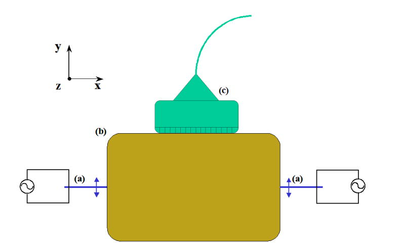
Experimental setup for the crawling wave estimator. Two bimorphs (a), in contact with the testing sample (b), vibrate in the direction perpendicular to the ultrasound transducer (c).

Under the plane wave assumption and considering a homogenous sample, the shear waves introduced by the right (W_right) and left (W_left) vibration sources can be described as follows:

$$W_{\mathit{right}}=e^{-{\alpha }_s(-x+D/2)}{e}^{-i(k_1(-x+D/2)-w_{1}t)}$$ (1)

$$W_{\mathit{left}}=e^{-{\alpha }_s(x+D/2)}{e}^{-i(k_2(x+D/2)-w_{2}t)}$$ (2)

where α_s is related to the attenuation of the wave in the sample, D is the distance between the sources, k₁ and k₂ are the wave numbers, and w₁ and w₂ are the frequencies of the vibration sources. In this particular case, w=w₁=w₂ and k=k₁=k₂. The resulting pattern is the superposition of the two waves. The squared signal envelope (|u(x,t)|²) will result in (Hoyt et al.):

$$\begin{array}{l}\mid u(x,t){\mid }^2=(W_{\mathit{right}}+W_{\mathit{left}})(W_{\mathit{right}}^{\ast }+W_{\mathit{left}}^{\ast })\\ \mid u(x,t){\mid }^2=e^{(D/2)}[e^{2{\alpha }_{s}x}+e^{-2{\alpha }_{s}x}+e^{2\mathit{ikx}}+e^{-2\mathit{ikx}}]\\ \mid u(x,t){\mid }^2=2e^{(D/2)}[cosh(2{\alpha }_{s}x)+cos(2\mathit{ikx})]\end{array}$$ (3)

The interference patterns described in equation 3 depend on a hyperbolic cosine and a cosine term. If a region far from the sources is analyzed, the hyperbolic cosine term can be dropped. Under such consideration, the spatial frequency of the interference patterns becomes 2k. Thus, the interference fringe spacing is half the shear wave wavelength (λ_s). The shear wave velocity (v_s) is estimated as:

$$v_s={\lambda }_{s}f$$ (4)

where f is controlled and given by the vibration sources and λ_s is measured from the image. In soft tissue, the relationship between Young’s modulus (E) and shear wave velocity can be approximated as follows:

$$E=3\rho {(v_s)}^2$$ (5)

where ρ is the mass density (approximately 1 g/cm³).

If there is a slight difference in frequency between the vibration sources, the interference patterns will slowly move towards the source with lower frequency. These moving patterns were termed “crawling waves.” The advantage of crawling waves is that they provide more observations to estimate the shear velocity of the testing sample, which is helpful in conditions of high tissue attenuation, small regions of interest, and poor signal-to-noise ratio.

The KVFD model

Previous studies have revealed that most biological soft tissues exhibit viscous behavior in addition to their better-known elastic properties. The viscoelastic properties of soft tissues are generally modeled as a combination of springs and dashpots because of their simplicity and ease of use. Caputo (1967) introduced fractional calculus into the field of viscoelasticity. He proposed a modified KV model which consists of a spring in parallel with a dashpot where the stress in the dashpot is equal to the fractional derivative of order α of the strain. Koeller (1984) first derived the stress relaxation function, with a time dependence t^−α in the function for the KVFD model. In a recent paper, Szabo and Wu (2000) described a frequency dependent power law for ultrasound attenuation in soft tissues, suggesting that many soft tissues can be modeled by a generalized KV model where the dashpot is replaced by a convolution operator (Chen and Holm 2003).

The KVFD model is a generalization of the KV model. In the KV model, stress in the dashpot is equal to the first derivative with respect to time of the strain. The KVFD model consists of a Hookean spring in parallel with a fractional derivative dashpot. The stress in the dashpot is equal to the fractional derivative of order α of the strain. This viscoelastic model contains three parameters: E₀, η, and α. E₀ refers to the relaxed elastic constant, η refers to the viscoelastic parameter, and α refers to the order of fractional derivative. The relationship between stress and strain in the KVFD model is given by the following constitutive differential equation:

$$\sigma (t)=E_0\epsilon (t)+\eta D^{\alpha }[\epsilon (t)]$$ (6)

where σ is stress, ε is strain, and t is time.

The fractional derivative operator D^α [ ] is defined by

$$D^{\alpha }[x(t)]=\frac{1}{\mathrm{\Gamma }(1-\alpha )}{\int }_0^t\frac{x^{\prime }(\tau )}{{(t-\tau )}^{\alpha }}d\tau$$ (7)

where Γ is the gamma function. For the KVFD model we restrict that 0 < α < 1.

Stress relaxation

Stress relaxation tests were used to characterize the viscoelastic behavior of the biological materials (Taylor et al. 2002). When a viscoelastic material is held at constant strain, the stress decreases with time. To develop a form of the relaxation function, the applied strain is modeled as a ramp of duration T_0, followed by a hold period of constant strain ε₀. So the strain function is:

$$\epsilon (t)=\{\begin{array}{ll}(t/T_0){\epsilon }_0\hfill & if\hspace{0.17em}0<t<T_0\hfill \\ {\epsilon }_0\hfill & \mathit{when}\hspace{0.17em}t\ge T_0\hfill \end{array}$$ (8)

Equation 8 has the Laplace transform:

$$\epsilon (s)=\frac{{\epsilon }_0}{s^2{T}_0}\left(1-e^{-s{T}_0}\right)$$ (9)

where s is the Laplace domain variable. By taking the Laplace transform of the constitutive equation 6, we get

$$\sigma (s)=E_0\epsilon (s)+\eta s^{\alpha }\epsilon (s)$$ (10)

We substitute equation 9 into equation 10 and obtain

$$\sigma (s)=E_0\frac{{\epsilon }_0}{s^2{T}_0}\left(1-e^{-s{T}_0}\right)+\eta \frac{{\epsilon }_0}{s^{2-\alpha }{T}_0}\left(1-e^{-s{T}_0}\right)$$ (11)

We apply inverse Laplace transform to both of the terms in equation 6

$$\sigma (t)=E_0\frac{{\epsilon }_0}{T_0}(tu(t)-(t-T_0)u(t-T_0))+\eta \frac{{\epsilon }_0}{\mathrm{\Gamma }(2-\alpha )T_0}\left(t^{1-\alpha }u(t)-{(t-T_0)}^{1-\alpha }u(t-T_0)\right)$$ (12)

where u () is the unit step function. Therefore, the stress response during the ramp period, 0 < t < T₀, is

$$\sigma (t)=E_0\frac{{\epsilon }_0}{T_0}t+\eta \frac{{\epsilon }_0}{\mathrm{\Gamma }(2-\alpha )T_0}{t}^{1-\alpha }$$ (13)

During the hold period t ≥ T₀, the response is obtained as

$$\sigma (t)=E_0{\epsilon }_0+\eta \frac{{\epsilon }_0}{\mathrm{\Gamma }(2-\alpha )T_0}\left(t^{1-\alpha }-{(t-T_0)}^{1-\alpha }\right)$$ (14)

Frequency response: complex modulus

Frequency domain response can be obtained from the time domain response and have a complex valued Young’s modulus at any frequency. Taking the Fourier transform of the constitutive equation 6 yields

$$\sigma (\omega )=E_0\epsilon (\omega )+\eta {(j\omega )}^{\alpha }\epsilon (\omega )$$ (15)

where ω is radian frequency and $j=\sqrt{-1}$. If the radian frequency is restricted to be positive, i.e., ω ≥ 0, equation 15 becomes

$$\sigma (\omega )=E_0\epsilon (\omega )+\eta e^{j\frac{\pi \alpha }{2}}{\omega }^{\alpha }\epsilon (\omega )$$ (16)

which is then factored to obtain the complex modulus E*(ω),

$$E\ast (\omega )=\frac{\sigma (\omega )}{\epsilon (\omega )}=\left[E_0+\eta cos\left(\frac{\pi \alpha }{2}\right){\omega }^{\alpha }\right]+j\left[\eta sin\left(\frac{\pi \alpha }{2}\right){\omega }^{\alpha }\right]$$ (17)

Since ω = 2πf, we rewrite equation 17 to express the complex Young’s modulus as a function of frequency (E*(f)).

$$E\ast (f)=\left[E_0+\eta cos\left(\frac{\pi \alpha }{2}\right){(2\pi f)}^{\alpha }\right]+j\left[\eta sin\left(\frac{\pi \alpha }{2}\right){(2\pi f)}^{\alpha }\right]$$ (18)

The magnitude of E *(f) can be expressed as

$$\mid E\ast (f)\mid =\sqrt{E_0^2+2E_0\eta cos\left(\frac{\pi \alpha }{2}\right){(2\pi f)}^{\alpha }+{\eta }^2{(2\pi f)}^{2\alpha }}$$ (19)

From equation 19 we can derive the storage modulus, E′(f), which is the real part of the complex modulus, and the loss modulus, E″(f), which is the imaginary part.

$$E^{\prime }(f)=E_0+\eta cos\left(\frac{\pi \alpha }{2}\right){(2\pi f)}^{\alpha }$$ (20)

$$E^{″}(f)=\eta sin\left(\frac{\pi \alpha }{2}\right){(2\pi f)}^{\alpha }$$ (21)

Figure 2 shows a diagram of the KVFD model (a), the typical data acquired from stress relaxation testing (b), and the typical magnitude of complex Young’s modulus as a function of frequency using equations 20 and 21 with the derived parameters E₀, η, and α for each case (c).

Figure 2.

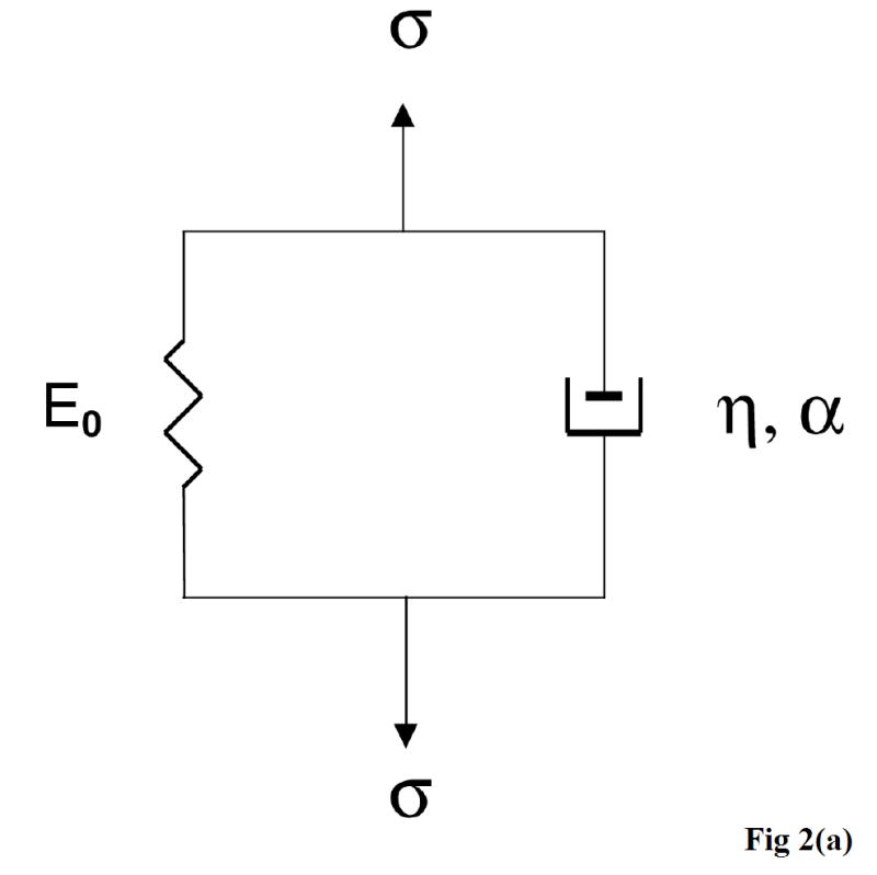
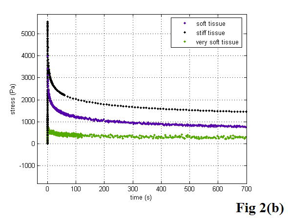
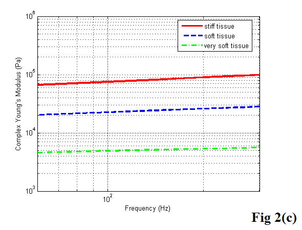
A diagram of the KVFD model (a), the typical stress relaxation curves obtained from different soft tissues (b), and the typical frequency dependent Young’s moduli of soft tissues with different stiffness (c).

MATERIALS AND METHODS

Tissue-mimicking gelatin phantom and specimen preparation

A cuboidal-shaped gelatin phantom (8 × 9 × 12 cm³) was produced for the preliminary study. The mechanical properties of the phantom are intended to mimic human soft tissue properties, especially Young’s modulus and speed of sound. The phantom was made from 1000 mL lab-made degassed, deionized water, 7.8% (w/w) food gelatin (Knoxx), 10% glycerol (v/v), 0.9% sodium chloride (w/w) and 0.5% graphite powder (w/w) as scatterers. The water was first heated to near boiling and then placed on the stirring plate, with a magnetic rod used to stir the water. The proper mass of gelatin powder was weighed and slowly added to the water. After most of the gelatin was dissolved, the solution was boiled again in a microwave oven with plastic wrap covering the container. Then the graphite powder was mixed into the solution. The mixture was cooled for about 50 minutes while stirring before the glycerol was finally mixed into the solution. The gelatin phantom was stored at approximately 4 °C overnight. It was then warmed up at room temperature (23 °C) for 4 hours before testing.

Whole fresh veal liver was obtained from a local butcher. Veal liver samples (approximately 8 × 8 × 6 cm³) were cut from the whole liver and refrigerated and stored in the lab-made degassed saline overnight. To make a thermal-treated sample, the liver chunk was heated at 70 °C for 50 minutes in degassed saline and then cooled to room temperature.

Human prostates were obtained from the Pathology Department at the University of Rochester Medical Center immediately following radical prostatectomy. The experimental protocol was approved by our institutional review board, and written informed consents were obtained from the two patients prior to radical prostatectomy to have in vitro imaging and mechanical testing performed. Here, we assume the prepared tissue samples are incompressible and elastically homogeneous.

Time-of-Flight (ToF) measurements on gelatin phantom

The shear wave ToF measurements were conducted on the gelatin phantom as an independent standard. During the experiment, the gelatin phantom was placed between a pair of bending motors (Piezo Systems, Cambridge, MA, USA); one functioned as a transmitter and the other as a receiver. From the transmitter-receiver distance and time lag of the signal, we can calculate the shear velocity in the phantom. Thus the Young’s modulus of the phantom can be estimated from the shear velocity using equation 5. A detailed description of the ToF measurement is presented in the earlier article (Wu et al. 2004).

Crawling wave estimator

Gelatin phantom, fresh and thermal-treated veal liver tissue samples, as well as excised prostate glands were placed between a pair of shear wave sources known as bimorphs (Piezo Systems, Cambridge, MA, USA). A GE Logiq 700 and a Logiq 9 Ultrasound Scanner (GE Ultrasound, Wauwatosa, WI, USA) were specially modified to perform the sonoelastography functions. Using those scanners, crawling wave movies were taken for each sample in a frequency range from 80 to 280 Hz. The wavelengths of the shear waves were measured from the movies using a model-based algorithm in MATLAB (The MathWorks, Inc., Natick, MA, USA). The shear wave velocity and Young’s modulus were estimated from the measurements as described in equations 4 and 5. The algorithm requires the user to input a region of interest (ROI). The user selects an ROI which is far from the vibration sources. Under this consideration, the interference patterns in the ROI look like parallel stripes (Figure 3a). A projection of the image over the axis perpendicular to the stripes is built and fit into a cosine model (Figure 3b):

Figure 3.

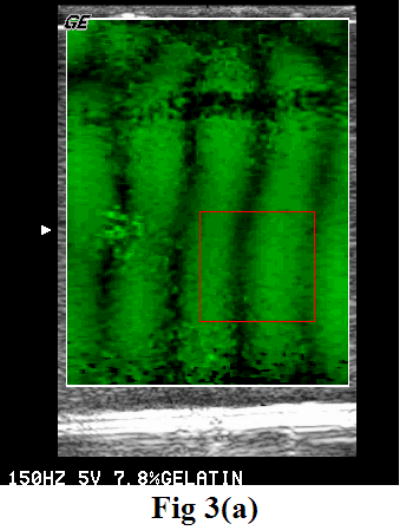
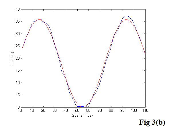
The user selects a region of interest (a) from the crawling wave movie. A projection is built from that region and fit into a cosine model (b). The image was acquired with a GE Logiq 700.

$$Y=Acos(2\pi k_{s}X-\theta )+D$$ (22)

Where Y is the projection built from the ROI; and A, k_s, θ, and D are the parameters of the model: amplitude, spatial frequency, phase, and offset, respectively. We note that k_s =1/λ_s and X is the independent spatial variable.

This curve fitting process was repeated for all the observations (i.e., each frame in the crawling wave movie). The final step was a cross optimization process performed over all observations. The estimated parameter (k_s) is used to calculate the shear wave velocity (v_s) and hence the elasticity modulus:

$$v_s=\frac{2f}{(1000)(k_s)(\mathit{pixel}\_mm)}$$ (23)

where f is the external vibration frequency and pixel_mm is the conversion factor from mm to pixels.

Mechanical measurement and curve fitting

Cylindrical cores (approximately 9 mm in diameter and 7 mm in length) were acquired from the gelatin phantom, fresh and thermal-treated liver tissues, and human prostates using a custom-made coring knife. The core samples were soaked in saline at room temperature for at least 30 minutes before mechanical testing. A 1/S mechanical device (MTS Systems Co., Eden Prairie, MN, USA) with a 5 Newton load cell was used to test the core samples. The upper and lower plates were coated with vegetable oil prior to testing. The core samples were put on the center of the lower testing plate. The top plate was used as a compressor and carefully positioned to fully contact the sample. After two minutes for tissue recovery, the uniaxial unconfined compression controlled by TestWorks 3.10 software (Software Research, Inc., San Francisco, CA, USA) was conducted to measure the time domain stress relaxation data at room temperature. The compression rate and the strain value were adjusted to 0.5 mm/sec and 5%, respectively. Throughout the test the stress required to maintain the compression was recorded over time. Tests lasted about 700 seconds. The resulting data consisted of a plot of the stress versus time under 5% strain. Multiple measurements were performed on each sample sequentially with 15-minute intervals in between. Samples were put back in saline during intervals to prevent dehydration. The prostate samples were later verified to be normal by histology in the Pathology Department at the University of Rochester Medical Center.

The stress relaxation curve of each sample during the hold period was fitted to the KVFD model using the MATLAB curve fitting toolkit. The trust-region method for nonlinear least squares fitting was applied on each curve. The averaged three model parameters, E₀, η, and α, were then obtained. Finally, the complex elastic modulus at any frequency was determined by the Fourier transform of the time domain response.

RESULTS

The gelatin phantom

CRE experimental results

The CRE experiments were performed on the 7.8% gelatin phantom. The two vibration sources were working at 100, 150, 200, 250, 300, and 350 Hz. Figures 3a and 4 show the interference patterns presented in the phantom at 150 Hz and 100 Hz. The differences in the wavelengths are apparent in the two images. The product of the wavelength and the signal frequency yields the shear wave velocities. The Young’s modulus of the phantom, therefore, was calculated at each frequency using equation 5, where a gelatin density of 1.05 g/cm³ was used.

Figure 4.

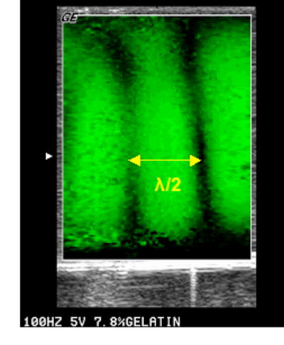
Sonoelastography image of shear wave interference patterns in the 7.8% gelatin phantom. Both sources vibrated at 100 Hz. The image was acquired with a GE Logiq 700.

Shear wave ToF results

On the gelatin phantom, shear wave ToF measurements were conducted. The distance between the tips of the transmitter and the receiver was 11.1 cm. When manually triggered at a certain frequency (100, 200, 300, or 400 Hz), one cycle of pulse at that frequency was transmitted into the phantom through the transmitter. The time lag between the received signal and the transmitted signal was 40.8 ms at 100 Hz. The shear wave velocity and the Young’s modulus were then calculated as 2.72 m/s and 23.32 kPa, respectively.

MM and curve fitting results

Four stress relaxation tests were conducted on the gelatin core sample. Figure 5 shows the typical stress relaxation curve of the sample at 5% strain. The curve was then fitted into the KVFD model. The parameters were applied in equation 19 to calculate the magnitude of complex Young’s modulus as a function of frequency. According to equations 20 and 21, the storage modulus (the elastic component) was greater than the loss modulus (the viscous component) by a factor of 10. In other words, the elastic part of the complex modulus dominated in the gelatin phantom. After that the shear velocity was estimated using equation 5.

Figure 5.

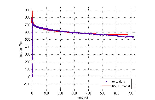
The stress relaxation of the 7.8% gelatin sample at 5% strain and its curve fit using the KVFD model. The dots are experimental data points. The solid line is the response predicted by the KVFD model. Model parameters for this fit are η = 15.39 kPa secα, α = 0.058, and E₀ close to 0 Pa (R² = 0.952).

Data comparison

Table 1 shows the results of the shear velocity and the Young’s modulus of the 7.8% gelatin phantom at 100, 200, and 300 Hz using the three different approaches described above. Taking the shear wave ToF results as the standard, the errors in Young’s modulus measurement on the gelatin phantom were less than 7% with the MM approach and less than 4% with the CRE approach, respectively. Graphical comparisons of the shear wave velocity and the Young’s modulus versus frequency measured with the three methods – CRE, MM, and ToF – can be seen in Figure 6. With the MM approach, each data point represents the averaged value over the total number of tests at that frequency. The error bars represent the standard deviation of the experimental data. Note that the magnitude of complex Young’s modulus was calculated from equation 19 and used here for comparison. To estimate the shear wave wavelength accurately with the CRE approach, we divided the distance from the start of the first detectable stripe to the last by the corresponding number of wavelengths. The measurement at each frequency was repeated several times. Since multiple measurements provided very consistent results with less than 1% error, we did not plot the standard deviation on the curve. The three curves in Figure 6 are highly congruent.

Table 1.

Summary of shear velocity and Young’s modulus measurements of the 7.8% gelatin sample using three methods: CRE, MM, and ToF. With the ToF method as the standard, the percentage of errors in the CRE and MM methods are presented in the parentheses.

Frequency (Hz)	Measured parameters	CRE	MM	ToF
100	vs (m/s)	2.7 (0.74%)	2.7 (1.10%)	2.7
	|E*| (kPa)	23.7 (1.42%)	22.7 (2.49%)	23.3
200	vs (m/s)	2.7 (1.49%)	2.8 (2.23%)	2.7
	|E*| (kPa)	22.1 (3.54%)	23.8 (3.89%)	22.9
300	vs (m/s)	2.7 (0.37%)	2.8 (3.35%)	2.7
	|E*| (kPa)	23.0 (0.66%)	24.4 (6.60%)	22.9

Figure 6.

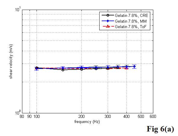
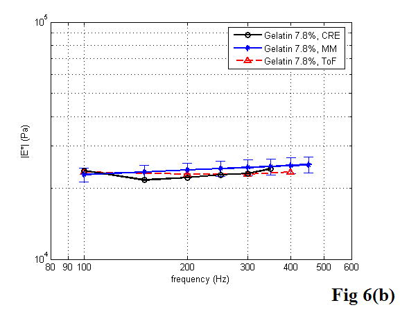
Comparison of the three approaches for estimation of the shear velocity (a) and the Young’s modulus (b) of the 7.8% gelatin phantom as a function of frequency.

The viscoelastic properties of soft tissues

To characterize soft tissue properties with the CRE approach, the crawling wave experiments were conducted on fresh veal liver, thermal-treated veal liver, and human prostate. Figure 7 shows one of the images taken from the crawling wave movies in the liver (a) and in human prostate (b). The measured moving velocity was used to calculate the shear velocity and the Young’s modulus for each tested object, taking liver and prostate density of 1 g/cm³.

Figure 7.

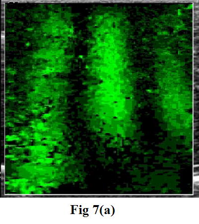
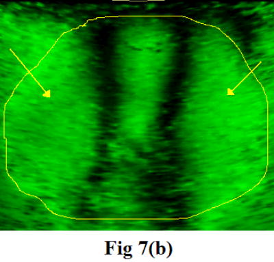
A snapshot of the moving patterns propagating through the fresh veal liver (a) imaged with a GE Logiq 700 and through human prostate (b) imaged with a GE Logiq 9. The frequencies of external vibration were 140 and 140.1 Hz for the liver, and 120 and 120.15 Hz for the prostate. The yellow outline in the prostate image is the profile of the prostate boundary delineated from the corresponding gray scale image. The arrows indicate the near-field artifact. Therefore, only a small ROI is visualized in the center of the image window.

Figure 8 shows the stress relaxation curves of a fresh liver sample and a prostate sample at 5% strain with curves fitted to the KVFD model. Each curve fitting had a correlation coefficient value larger than 0.98, demonstrating that the stress relaxation curves were fitted very well to the KVFD model. It was also observed that the stress needs quite a long time to reach the equilibrium status, indicating that tissues like fresh liver and normal prostate are very soft viscoelastic materials. Table 2 summarizes the best-fit parameters and correlation coefficient (R²) values for all of the examined samples. The magnitude of complex Young’s modulus in the frequency domain was determined with those model parameters. However, E₀ was not included in the table because the curve fitting results provided E₀ values close to zero. This finding indicates that E₀ does not contribute significantly to the overall Young’s modulus in those cases. Using equations 20 and 21, the storage modulus was calculated as greater than the loss modulus by a factor of 4.5 for the fresh veal liver and a factor of 3.5 for the thermal-treated liver in the tested frequency range. The ratio of the storage modulus to the loss modulus for the prostate was about 2.5. The shear velocity was estimated according to equation 5.

Figure 8.

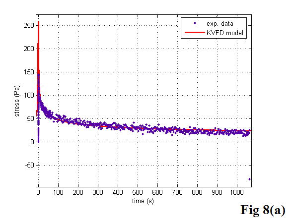
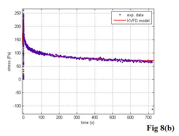
The stress relaxation curves of a liver sample (a) and a prostate sample (b). The curves were fitted to the KVFD model. The dots are experimental data points. The solid line is the response predicted by the KVFD model. The R² values of the two curve fittings are 0.983 and 0.984, respectively.

Table 2.

Best-fit parameters for tested samples using the KVFD model.

Sample type	No. of tests	η (kPa s α)	α	R2
7.8% Gelatin	4	15100±286	0.064±0.008	0.958
Veal liver #1	3	7820±1050	0.111±0.020	0.927
Veal liver #2	3	5130±885	0.122±0.033	0.977
Veal liver #3	3	4730±361	0.274±0.025	0.983
Thermal-treated liver #1	4	102000±15400	0.180±0.024	0.998
Thermal-treated liver #2	4	145000±23600	0.150±0.021	0.999
Human prostate #1	3	3480±2	0.219±0.037	0.944
Human prostate #2	4	5110±1590	0.238±0.045	0.973

A comparison between the CRE results and the MM results of various soft tissues is illustrated in Figure 9, including the estimation of the Young’s modulus as a function of frequency. Once again, the MM approach provided the average magnitude of complex Young’s modulus with the standard deviation. In the CRE approach, the frequency range was determined by the visibility of the crawling waves in different tissues.

Figure 9.

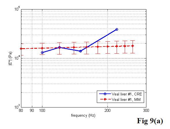
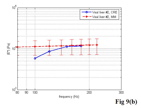
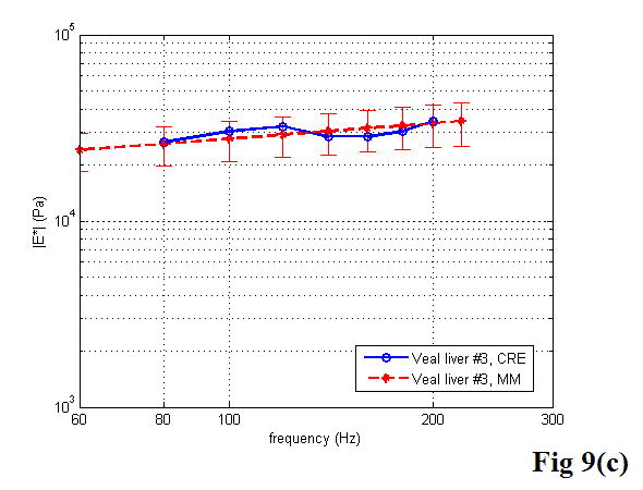
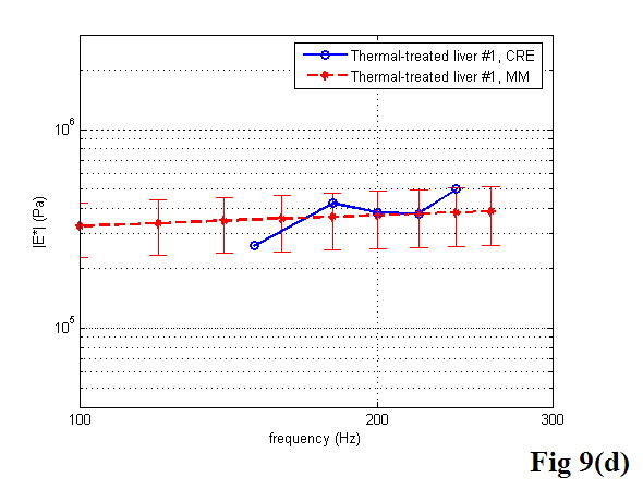
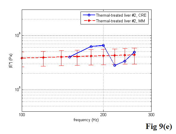
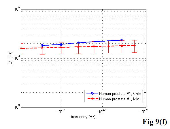
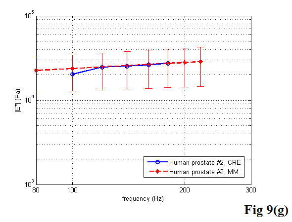
Comparison of the CRE results and the MM results on fresh veal liver (a–c), thermal-treated liver (d, e), and normal human prostate (f, g) tissues. The magnitude of complex Young’s modulus is plotted against frequency for each soft tissue sample.

DISCUSSION AND CONCLUSIONS

When estimating the shear velocity using CRE, we observed a frequency lower limit exists that is dependent on the material properties and imaging field area. Below this frequency limit, the wavelength is too long compared to the width of the image window, and only a portion of one wavelength displays in the image window. On the other hand, a frequency upper limit also exists since viscoelastic materials’ shear wave attenuation generally increases with frequency. Above this frequency limit, the energy of the two facing waves dies out before they significantly interfere. For soft tissues like liver and prostate, the approach presented in this paper, using crawling wave movies, is especially useful since the medium is very attenuating, and only a few interference fringes (providing a small ROI) can be visualized in the center of the image window (Figure 7b). This technique takes advantage of the different observations (each frame in the movie) that provide more information to fit into the cosine model, and then gives us reliable measurements of soft tissue properties. In addition, the precision of this imaging technique relies on the image contrast and resolution; the detailed analysis is beyond the scope of this paper.

In the mechanical testing experiments, several issues should be considered and handled properly to reduce the variability of measurement on each sample. For example, it is necessary to section the upper and lower surfaces of the cylindrical sample as parallel and as flat as possible for compression tests. However, this requirement is hard to achieve, especially when the sample is very soft, such as fresh liver and prostate. Two blades in parallel were used for sample sectioning. Multiple tests were conducted on each sample. The results were averaged, and the standard deviation was given to assess the repeatability of the stress relaxation tests. The detailed analysis indicated that the variability due to the imperfect shape of the sample was relatively small, as we expected. Another problem in the experiment was dehydration of the sample. To minimize the dehydration effect, the side of each sample was coated with a thin layer of Vaseline. This process was found to be effective during the tests.

There are three important parameters in the KVFD model: E₀, η, and α, as mentioned previously. Interestingly, curve-fitting results always gave the examined soft tissues E₀ values approaching zero. To extract the relaxed spring parameter E₀, we note that in equation 14,σ (∞) = E₀ε₀, meaning when equilibrium is reached, E₀ is the value of stress σ divided by the applied strain, ε₀. As we know, the stress of a perfectly elastic material would be constant with time, while for a Newtonian fluid the stress level would relax rapidly to zero. In our stress relaxation tests, the stress response did not reach the equilibrium status for a long time and the stress level was approaching zero asymptotically, indicating the tested soft tissues are fluid-like viscoelastic materials. To further confirm this phenomenon, several long span tests were performed on liver and cancerous prostate tissues. Figure 10 shows the stress responses of those biological soft tissues during very long tests. Although we could not record the stress relaxation curves long enough to reach the plateau due to the limit of the MTS system, we still observed that the stress levels reached zero. Therefore, parameter E₀ in the KVFD model was observed to have a relatively small value and did not contribute significantly to the overall elasticity in our tests. However, for other soft tissues, E₀ is not always negligible; this will be discussed in a later paper.

Figure 10.

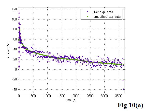
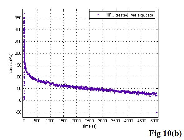
The stress relaxation of veal liver (a) and thermal-treated liver (b) over long times. The liver data is noisy because the stress levels were well below the full scale value of the load cell. We smoothed the data with the MATLAB “robust lowess” method and a span of 0.25.

With 0 < α < 1, the fractional derivative dashpot consists of not only the viscous component but also the elastic component, with the modulus having both real and imaginary components. Therefore, even when E₀ is a very small number close to zero, the storage modulus, corresponding to the elastic behavior of the tested soft tissue, is still greater than the loss modulus, the viscous response of the tissue, by a factor of 2.5 or more. The value of α is noticeably related to the viscosity of the material, since the loss modulus increases with the increase of α. The same tendency was found in the slope of the Young’s modulus versus frequency curve, which increases with rising α.

By comparing the results of the two approaches, we did find that the derived Young’s moduli were nearly congruent on soft tissue characterization. Although we assumed that tissue samples were homogeneous, it is not always true practically. The inhomogeneity affected our measurements to some extent. Therefore, on prostate sample 2, we took the same position in the gland for both measurements (Figure 11). The results were closer, with the difference of the Young’s modulus less than 10% in a range from 100 to 180 Hz. The average difference of the Young’s modulus measured by the two approaches was less than 12.5% at 150 Hz for all of the examined tissues. However, we observed that there was noticeable liver-to-liver variability in the viscoelastic properties. For example, veal liver sample 3 measured with the MM and the CRE approaches was about twice as stiff (29.9 ± 1.2 kPa) as veal liver samples 1 and 2 (12.9 ± 3.8 kPa) at 120 Hz. This stiffness difference can be caused by the animals’ age and process conditions such as time and temperature, etc. For thermal-treated livers and normal human prostates, the individual stiffness variations were much smaller than that in fresh veal livers. For instance, the Young’s modulus of thermal-treated livers measured with the two approaches was 349.4 ± 73.0 kPa at 150 Hz, and that of human prostates was 21.0 ± 5.0 kPa at 180 Hz.

Figure 11.

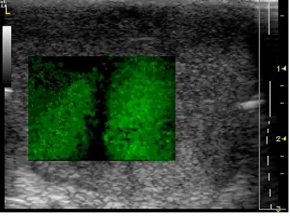
The crawling waves propagate through the region of interest in the prostate. After imaging, the core sample was taken in the same position for a better comparison.

In the present study, the CRE measurements were compared with stress relaxation tests with the use of the viscoelastic KVFD model. The CRE versus MM results of the same sample were plotted directly against each other. Our CRE approach provided shear wave interference patterns from which the shear wave velocity can be determined and hence the Young’s modulus can be obtained. The MM approach along with the KVFD modeling provided the complex Young’s modulus of the soft tissue from which both elastic and viscous behavior can be extracted, and the shear wave velocity can be calculated for comparison purposes. We observed that both liver and prostate tissues have frequency dependent Young’s moduli that slightly increase with frequency in the tested range, which is similar to the findings reported by Shau et al. (2001). Our results on liver tissue characterization are comparable with the data reported by several groups such as Kruse et al. (2000), Liu and Bilston (2000), and Kiss et al. (2004) as mentioned earlier. Although different animal livers and testing methods were used, they did observe that liver is viscoelastic and has a frequency dependent modulus over a tested frequency range. The reports of prostate mechanical properties are fewer. Kemper et al. (2004) investigated the shear stiffness of normal human prostates with an in vivo MRE technique. Their results are in a similar range as ours. In contrast, Krouskop et al. (1998) applied dynamic testing at low frequencies (0.1 to 4 Hz) on human prostate specimens. Their results were higher than ours by a factor of 5. Phipps et al. (2005b) correlated the Young’s modulus with the percentage of prostatic smooth muscle. However, a wide range of the Young’s modulus from 40 to 140 kPa was described in that article.

In summary, this study achieves three important accomplishments. First, we characterized soft tissue properties with two independent techniques: the crawling wave estimator and mechanical stress relaxation with results fit to the KVFD model. Our investigation has indicated that the CRE technique is a feasible real-time imaging measurement for soft tissue characterization within a certain frequency range. The stress relaxation test produces repeatable results which fit well to the KVFD model (R² > 0.93). The complex Young’s modulus estimated by the MM technique may provide useful information, such as tissue viscosity, to advance tissue characterization. Second, this paper is the first attempt to compare these two quantitative measurements of various soft tissues. In previous studies, the two techniques were investigated individually on a gelatin phantom or liver tissue. The validity of those results, however, had not been thoroughly studied. The congruence of the two methods on liver and prostate tissue characterization confirms their robustness and suggests they can be used to investigate viscoelastic properties of other soft tissues. Particularly, as an imaging modality, the CRE technique has the potential to be utilized for in vivo soft tissue measurements, offering a simple and effective real-time approach to quantify tissue properties. Finally, the results contribute to the limited information in the literature on the viscoelastic properties of soft tissues such as veal liver and human prostate.

References

- Arbogast KB, Margulies SS. Material characterization of the brainstem from oscillatory shear tests. J Biomech. 1998;31:801–807. doi: 10.1016/s0021-9290(98)00068-2. [DOI] [PubMed] [Google Scholar]
- Bensamoun SF, Ringleb SI, Littrell L, Chen Q, Brennan M, Ehman RL, An KN. Determination of thigh muscle stiffness using magnetic resonance elastography. J Magn Reson Imaging. 2006;23:242–247. doi: 10.1002/jmri.20487. [DOI] [PubMed] [Google Scholar]
- Bercoff J, Tanter M, Fink M. Supersonic shear imaging: a new technique for soft tissue elasticity mapping. IEEE Trans Ultrason Ferroelectr Freq Control. 2004;51:396–409. doi: 10.1109/tuffc.2004.1295425. [DOI] [PubMed] [Google Scholar]
- Bishop J, Poole G, Leitch M, Plewes DB. Magnetic resonance imaging of shear wave propagation in excised tissue. J Magn Reson Imaging. 1998;8:1257–1265. doi: 10.1002/jmri.1880080613. [DOI] [PubMed] [Google Scholar]
- Caputo M. Linear models of dissipation whose q is almost frequency independent-II. Geophys J R Astr Soc. 1967;13:529–539. [Google Scholar]
- Catheline S, Wu F, Fink M. A solution to diffraction biases in sonoelasticity: the acoustic impulse technique. J Acoust Soc Am. 1999;105:2941–2950. doi: 10.1121/1.426907. [DOI] [PubMed] [Google Scholar]
- Chen EJ, Novakofski J, Jenkins WK, OBrien WD. Young’s modulus measurements of soft tissues with application to elasticity imaging. Ieee Transactions on Ultrasonics Ferroelectrics and Frequency Control. 1996;43:191–194. [Google Scholar]
- Chen W, Holm S. Modified Szabo’s wave equation models for lossy media obeying frequency power law. J Acoust Soc Am. 2003;114:2570–2574. doi: 10.1121/1.1621392. [DOI] [PubMed] [Google Scholar]
- Darvish KK, Crandall JR. Nonlinear viscoelastic effects in oscillatory shear deformation of brain tissue. Med Eng Phys. 2001;23:633–645. doi: 10.1016/s1350-4533(01)00101-1. [DOI] [PubMed] [Google Scholar]
- Dunn MG, Silver FH. Viscoelastic behavior of human connective tissues: relative contribution of viscous and elastic components. Connect Tissue Res. 1983;12:59–70. doi: 10.3109/03008208309005612. [DOI] [PubMed] [Google Scholar]
- Erkamp RQ, Wiggins P, Skovoroda AR, Emelianov SY, O’Donnell M. Measuring the elastic modulus of small tissue samples. Ultrason Imaging. 1998;20:17–28. doi: 10.1177/016173469802000102. [DOI] [PubMed] [Google Scholar]
- Fatemi M, Greenleaf JF. Ultrasound-stimulated vibro-acoustic spectrography. Science. 1998;280:82–85. doi: 10.1126/science.280.5360.82. [DOI] [PubMed] [Google Scholar]
- Fowlkes JB, Emelianov SY, Pipe JG, Skovoroda AR, Carson PL, Adler RS, Sarvazyan AP. Magnetic-resonance imaging techniques for detection of elasticity variation. Med Phys. 1995;22:1771–1778. doi: 10.1118/1.597633. [DOI] [PubMed] [Google Scholar]
- Fung YC. Biomechanics: mechanical properties of living tissues. New York: Springer-Verlag; 1993. [Google Scholar]
- Hamhaber U, Grieshaber FA, Nagel JH, Klose U. Comparison of quantitative shear wave MR-elastography with mechanical compression tests. Magn Reson Med. 2003;49:71–77. doi: 10.1002/mrm.10343. [DOI] [PubMed] [Google Scholar]
- Hof AL. Muscle mechanics and neuromuscular control. J Biomech. 2003;36:1031–1038. doi: 10.1016/s0021-9290(03)00036-8. [DOI] [PubMed] [Google Scholar]
- Hoyt K, Castaneda B, Zhang M, Rubens DJ, Parker KJ. Real-time shear velocity imaging using sonoelasgraphic techniques. Ultrasound Med Biol. doi: 10.1016/j.ultrasmedbio.2007.01.009. in press. [DOI] [PubMed] [Google Scholar]
- Huang CY, Wang VM, Pawluk RJ, Bucchieri JS, Levine WN, Bigliani LU, Mow VC, Flatow EL. Inhomogeneous mechanical behavior of the human supraspinatus tendon under uniaxial loading. J Orthop Res. 2005;23:924–930. doi: 10.1016/j.orthres.2004.02.016. [DOI] [PubMed] [Google Scholar]
- Huang SR, Lerner RM, Parker KJ. On estimating the amplitude of harmonic vibration from the Doppler spectrum of reflected signals. Journal of the Acoustical Society of America. 1990;88:2702–2712. [Google Scholar]
- Kemper J, Sinkus R, Lorenzen J, Nolte-Ernsting C, Stork A, Adam G. MR elastography of the prostate: initial in-vivo application. Rofo. 2004;176:1094–1099. doi: 10.1055/s-2004-813279. [DOI] [PubMed] [Google Scholar]
- Kiss MZ, Varghese T, Hall TJ. Viscoelastic characterization of in vitro canine tissue. Phys Med Biol. 2004;49:4207–4218. doi: 10.1088/0031-9155/49/18/002. [DOI] [PMC free article] [PubMed] [Google Scholar]
- Klein TJ, Chaudhry M, Bae WC, Sah RL. Depth-dependent biomechanical and biochemical properties of fetal, newborn, and tissue-engineered articular cartilage. J Biomech. 2005 doi: 10.1016/j.jbiomech.2005.11.002. [DOI] [PubMed] [Google Scholar]
- Koeller RC. Applications of fractional calculus to the theory of viscoelasticity. Journal of Applied Mechanics-Transactions of the Asme. 1984;51:299–307. [Google Scholar]
- Krouskop TA, Dougherty DR, Vinson FS. A pulsed Doppler ultrasonic system for making noninvasive measurements of the mechanical properties of soft tissue. J Rehabil Res Dev. 1987;24:1–8. [PubMed] [Google Scholar]
- Krouskop TA, Wheeler TM, Kallel F, Garra BS, Hall T. Elastic moduli of breast and prostate tissues under compression. Ultrason Imaging. 1998;20:260–274. doi: 10.1177/016173469802000403. [DOI] [PubMed] [Google Scholar]
- Kruse SA, Smith JA, Lawrence AJ, Dresner MA, Manduca A, Greenleaf JF, Ehman RL. Tissue characterization using magnetic resonance elastography: preliminary results. Phys Med Biol. 2000;45:1579–1590. doi: 10.1088/0031-9155/45/6/313. [DOI] [PubMed] [Google Scholar]
- Kuo PL, Li PC, Li ML. Elastic properties of tendon measured by two different approaches. Ultrasound Med Biol. 2001;27:1275–1284. doi: 10.1016/s0301-5629(01)00442-2. [DOI] [PubMed] [Google Scholar]
- Lally C, Reid AJ, Prendergast PJ. Elastic behavior of porcine coronary artery tissue under uniaxial and equibiaxial tension. Ann Biomed Eng. 2004;32:1355–1364. doi: 10.1114/b:abme.0000042224.23927.ce. [DOI] [PubMed] [Google Scholar]
- Lerner RM, Parker KJ, Holen J, Gramiak R, Waag RC. Sonoelasticity: medical elasticity images derived from ultrasound signals in mechanically vibrated targets. Acoustical Imaging. 1988;16:317–327. [Google Scholar]
- Liu Z, Bilston L. On the viscoelastic character of liver tissue: experiments and modelling of the linear behaviour. Biorheology. 2000;37:191–201. [PubMed] [Google Scholar]
- Muthupillai R, Lomas DJ, Rossman PJ, Greenleaf JF, Manduca A, Ehman RL. Magnetic resonance elastography by direct visualization of propagating acoustic strain waves. Science. 1995;269:1854–1857. doi: 10.1126/science.7569924. [DOI] [PubMed] [Google Scholar]
- Nasseri S, Bilston LE, Phan-Thien N. Viscoelastic properties of pig kidney in shear, experimental results and modelling. Rheologica Acta. 2002;41:180–192. [Google Scholar]
- Nightingale KR, Palmeri ML, Nightingale RW, Trahey GE. On the feasibility of remote palpation using acoustic radiation force. J Acoust Soc Am. 2001;110:625–634. doi: 10.1121/1.1378344. [DOI] [PubMed] [Google Scholar]
- Ophir J, Cespedes I, Ponnekanti H, Yazdi Y, Li X. Elastography: a quantitative method for imaging the elasticity of biological tissues. Ultrason Imaging. 1991;13:111–134. doi: 10.1177/016173469101300201. [DOI] [PubMed] [Google Scholar]
- Papazoglou S, Rump J, Braun J, Sack I. Shear wave group velocity inversion in MR elastography of human skeletal muscle. Magn Reson Med. 2006;56:489–497. doi: 10.1002/mrm.20993. [DOI] [PubMed] [Google Scholar]
- Parker KJ, Huang SR, Musulin RA, Lerner RM. Tissue response to mechanical vibrations for “sonoelasticity imaging”. Ultrasound Med Biol. 1990;16:241–246. doi: 10.1016/0301-5629(90)90003-u. [DOI] [PubMed] [Google Scholar]
- Phipps S, Yang TH, Habib FK, Reuben RL, McNeill SA. Measurement of the mechanical characteristics of benign prostatic tissue: a novel method for assessing benign prostatic disease. Urology. 2005a;65:1024–1028. doi: 10.1016/j.urology.2004.12.022. [DOI] [PubMed] [Google Scholar]
- Phipps S, Yang TH, Habib FK, Reuben RL, McNeill SA. Measurement of tissue mechanical characteristics to distinguish between benign and malignant prostatic disease. Urology. 2005b;66:447–450. doi: 10.1016/j.urology.2005.03.017. [DOI] [PubMed] [Google Scholar]
- Plewes DB, Betty I, Urchuk SN, Soutar I. Visualizing tissue compliance with MR imaging. J Magn Reson Imaging. 1995;5:733–738. doi: 10.1002/jmri.1880050620. [DOI] [PubMed] [Google Scholar]
- Provenzano PP, Lakes RS, Corr DT, R R., Jr Application of nonlinear viscoelastic models to describe ligament behavior. Biomech Model Mechanobiol. 2002;1:45–57. doi: 10.1007/s10237-002-0004-1. [DOI] [PubMed] [Google Scholar]
- Ringleb SI, Chen Q, Lake DS, Manduca A, Ehman RL, An KN. Quantitative shear wave magnetic resonance elastography: comparison to a dynamic shear material test. Magn Reson Med. 2005;53:1197–1201. doi: 10.1002/mrm.20449. [DOI] [PubMed] [Google Scholar]
- Rouviere O, Yin M, Dresner MA, Rossman PJ, Burgart LJ, Fidler JL, Ehman RL. MR elastography of the liver: preliminary results. Radiology. 2006;240:440–448. doi: 10.1148/radiol.2402050606. [DOI] [PubMed] [Google Scholar]
- Sanada M, Ebara M, Fukuda H, Yoshikawa M, Sugiura N, Saisho H, Yamakoshi Y, Ohmura K, Kobayashi A, Kondoh F. Clinical evaluation of sonoelasticity measurement in liver using ultrasonic imaging of internal forced low-frequency vibration. Ultrasound Med Biol. 2000;26:1455–1460. doi: 10.1016/s0301-5629(00)00307-0. [DOI] [PubMed] [Google Scholar]
- Sandrin L, Tanter M, Catheline S, Fink M. Shear modulus imaging with 2-D transient elastography. IEEE Trans Ultrason Ferroelectr Freq Control. 2002a;49:426–435. doi: 10.1109/58.996560. [DOI] [PubMed] [Google Scholar]
- Sandrin L, Tanter M, Gennisson JL, Catheline S, Fink M. Shear elasticity probe for soft tissues with 1-D transient elastography. IEEE Trans Ultrason Ferroelectr Freq Control. 2002b;49:436–446. doi: 10.1109/58.996561. [DOI] [PubMed] [Google Scholar]
- Sandrin L, Fourquet B, Hasquenoph JM, Yon S, Fournier C, Mal F, Christidis C, Ziol M, Poulet B, Kazemi F, Beaugrand M, Palau R. Transient elastography: a new noninvasive method for assessment of hepatic fibrosis. Ultrasound Med Biol. 2003;29:1705–1713. doi: 10.1016/j.ultrasmedbio.2003.07.001. [DOI] [PubMed] [Google Scholar]
- Sarvazyan AP, Rudenko OV, Swanson SD, Fowlkes JB, Emelianov SY. Shear wave elasticity imaging: a new ultrasonic technology of medical diagnostics. Ultrasound Med Biol. 1998;24:1419–1435. doi: 10.1016/s0301-5629(98)00110-0. [DOI] [PubMed] [Google Scholar]
- Shau YW, Wang CL, Hsieh FJ, Hsiao TY. Noninvasive assessment of vocal fold mucosal wave velocity using color doppler imaging. Ultrasound Med Biol. 2001;27:1451–1460. doi: 10.1016/s0301-5629(01)00453-7. [DOI] [PubMed] [Google Scholar]
- Silver FH, Horvath I, Foran DJ. Viscoelasticity of the vessel wall: the role of collagen and elastic fibers. Crit Rev Biomed Eng. 2001;29:279–301. doi: 10.1615/critrevbiomedeng.v29.i3.10. [DOI] [PubMed] [Google Scholar]
- Sinkus R, Tanter M, Xydeas T, Catheline S, Bercoff J, Fink M. Viscoelastic shear properties of in vivo breast lesions measured by MR elastography. Magn Reson Imaging. 2005;23:159–165. doi: 10.1016/j.mri.2004.11.060. [DOI] [PubMed] [Google Scholar]
- Snedeker JG, Niederer P, Schmidlin FR, Farshad M, Demetropoulos CK, Lee JB, Yang KH. Strain-rate dependent material properties of the porcine and human kidney capsule. J Biomech. 2005;38:1011–1021. doi: 10.1016/j.jbiomech.2004.05.036. [DOI] [PubMed] [Google Scholar]
- Suki B, Barabasi AL, Lutchen KR. Lung tissue viscoelasticity: a mathematical framework and its molecular basis. J Appl Physiol. 1994;76:2749–2759. doi: 10.1152/jappl.1994.76.6.2749. [DOI] [PubMed] [Google Scholar]
- Szabo TL, Wu J. A model for longitudinal and shear wave propagation in viscoelastic media. J Acoust Soc Am. 2000;107:2437–2446. doi: 10.1121/1.428630. [DOI] [PubMed] [Google Scholar]
- Taylor LS, Lerner AL, Rubens DJ, Parker KJ. A Kelvin-Voigt fractional derivative model for viscoelastic characterization of liver tissue. In: Scott EP, editor. ASME Int. Mechanical Engineering Congress and Exposition; New Orleans, LA. 2002. [Google Scholar]
- Wu JZ, Dong RG, Smutz WP, Schopper AW. Nonlinear and viscoelastic characteristics of skin under compression: experiment and analysis. Biomed Mater Eng. 2003;13:373–385. [PubMed] [Google Scholar]
- Wu Z, Taylor LS, Rubens DJ, Parker KJ. Sonoelastographic imaging of interference patterns for estimation of the shear velocity of homogeneous biomaterials. Phys Med Biol. 2004;49:911–922. doi: 10.1088/0031-9155/49/6/003. [DOI] [PubMed] [Google Scholar]
- Yamakoshi Y, Sato J, Sato T. Ultrasonic-imaging of internal vibration of soft-tissue under forced vibration. IEEE Transactions on Ultrasonics Ferroelectrics and Frequency Control. 1990;37:45–53. doi: 10.1109/58.46969. [DOI] [PubMed] [Google Scholar]
- Yang X, Church CC. A simple viscoelastic model for soft tissues in the frequency range 6–20 MHz. IEEE Trans Ultrason Ferroelectr Freq Control. 2006;53:1404–1411. doi: 10.1109/tuffc.2006.1665097. [DOI] [PubMed] [Google Scholar]
- Yeh WC, Li PC, Jeng YM, Hsu HC, Kuo PL, Li ML, Yang PM, Lee PH. Elastic modulus measurements of human liver and correlation with pathology. Ultrasound Med Biol. 2002;28:467–474. doi: 10.1016/s0301-5629(02)00489-1. [DOI] [PubMed] [Google Scholar]