Lure-similarity affects visual episodic recognition: Detailed tests of a noisy exemplar model

Abstract

Summed-similarity models of visual episodic-recognition memory successfully predict the variation in false-alarm rates across different test items. With data averaged across subjects, Kahana and Sekuler (2002) demonstrated that subjects' performance appears to change along with the mean similarity among study items; with high interstimulus similarity, subjects were less likely to commit false alarms to similar lures. We examined this effect in detail by systematically varying the coordinates of study and test items along a critical stimulus dimension and measuring memory performance at each point. To reduce uncontrolled variance associated with individual differences in vision, the coordinates of study and test items were scaled according to each subject's discrimination threshold. Fitting each of four summed-similarity models to the individual subjects' data demonstrated a clear superiority for models that take account of inter-item similarity on a trialwise basis.

Kahana and Sekuler (2002) adapted Sternberg's procedure (1966, 1975) to study episodic recognition memory for series of textures, which were created by linearly summing sinusoidal gratings. This adaptation made it possible to quantify and characterize interference in memory among successively presented stimuli. Unlike semantically rich stimuli, such as words or images of recognizable and nameable objects, multidimensional textures are not burdened by the complexities of extralaboratory associations, and they resist symbolic coding (Della-Maggiore et al., 2000; Hwang et al., 2005). Because of their well-defined, natural metric representations in a low-dimensional space (Kahana & Bennett, 1994), compound grating stimuli facilitate manipulation of interitem similarity relations, which are important determinants of visual episodic recognition (Kahana & Sekuler, 2002; Zhou, Kahana, & Sekuler, 2004; Sekuler, Kahana, McLaughlin, Golomb, & Wingfield, 2005). The availability of a natural stimulus metric for defining similarity relations among items enables detailed mathematical accounts of recognition memory to be applied to results from individual stimulus lists.

Using Nosofsky's (1984, 1986) Generalized Context Model (GCM) as our starting point, we developed NEMO, a Noisy Exemplar Model, which combines core aspects of GCM with significant new assumptions. First, NEMO follows the tradition of multidimensional signal-detection theory (e.g., Ashby & Maddox, 1998) in assuming that stimulus representations are coded in a noisy manner, with a different level of noise associated with each dimension. Second, NEMO augments the summed-similarity framework of item recognition (Brockdorff & Lamberts, 2000; Clark & Gronlund, 1996; Humphreys, Pike, Bain, & Tehan, 1989; Lamberts, Brockdorff, & Heit, 2003; Nosofsky, 1991, 1992) with the idea that within-list summed similarity (not just probe-to-list-item similarity) influences recognition decisions. In fitting NEMO to data from two experiments, Kahana and Sekuler (2002) found that subjects were more likely to say yes to lures following study of lists whose items have low interitem similarity than to lures following lists whose items have high interitem similarity. Subjects appear to interpret probe-to-list similarity in light of within-list similarity, with greater list homogeneity leading to a greater tendency to reject lures that are similar to one or more of the studied items. The impact of within-list similarity was confirmed by Nosofsky and Kantner (2006), using color patches as stimuli.

In vision research, many studies focus on the individual performance of a small number of subjects. In contrast, memory research tends to focus on performance averaged across subjects. The statistical advantage of averaging is obvious, but this advantage extracts a toll. It can introduce qualitative changes into the pattern of data, thereby distorting the outcome of quantitative modeling (e.g., Maddox, 1999). Although we subscribe to the goal of understanding the visual episodic-recognition performance of individual subjects, previous datasets, including our own, were not large enough to support meaningful modeling of individual subjects' data. Therefore, our model-driven analyses to date have all been done on averaged data. The experiment described below was designed to produce data sufficient to support modeling on an individual-subject level.

Our goal in this paper is to compare the fits of a suite of NEMO variants to individual subjects' data, where the latter are generated using the roving probe paradigm (Zhou et al., 2004). In the roving probe paradigm, subjects study a short list of stimuli that vary along one (or more) dimensions for a subsequent recognition memory test. By randomly selecting test probes from a uniform distribution along the same stimulus dimension as the studied items, the roving probe method can reveal the parametric relation between the probability of subjects' yes responses and the metric properties of the probe stimulus. We first present the experimental study that generated a dataset suitable for model-fits to individual subjects' results. We then describe the NEMO model in detail, including minor changes from our earlier implementation (Kahana & Sekuler, 2002). The third section of the paper presents fits of four variants of NEMO to individual subjects' data, and discusses the contributions of the various core modeling assumptions to obtaining a good quantitative fit. Finally, we discuss the limitations of NEMO's current version, and ways that the model could be extended to account for a broader range of important attributes of perceptual memory.

Methods

Participants

Participants were five male and five female volunteers whose ages ranged from 19 to 30 years. They had normal or corrected-to-normal visual acuity as measured with Snellen targets, and normal contrast sensitivity as measured with Pelli-Robson charts (Pelli, Robson, & Wilkins, 1988).

Apparatus

Stimuli were generated and displayed using Matlab 5 and extensions from the Psychophysics and Video Toolboxes (Brainard, 1997; Pelli, 1997). Stimuli were presented on a 14-inch CRT computer monitor with a refresh rate of 95 Hz and a screen resolution of 800 by 600 pixels. Routines from the Video Toolbox were used to calibrate and linearize the display. Mean screen luminance was maintained at 36 cd/m².

Stimuli

On each trial, three compound gratings, s₁, s₂, and p, were presented sequentially. At the start of each trial, a fixation point was centered on the screen for 750 msec. The fixation point was followed by a 750-msec period of uniform luminance. s₁, then s₂, followed, each for 1000 msec, separated by an interstimulus interval (ISI) of 1000 msec. During the ISI, the display area was filled with uniform luminance (36 cd/m²). Finally, 1000 msec after s₂, p was presented and remained visible until the observer responded. p disappeared 1000 msec after its onset if the observer did not respond in such a period. A sample trial is schematized in Figure 1.

Figure 1.

A schematized example of a trial. The events, whose durations are indicated on the timeline at the bottom of the figure, begin with a fixation point, which is then succeeded by s₁, s₂, and p. In this example, p is a lure, differing from both s₁ and s₂. The correct response, therefore, would be no.

In each stimulus, one vertical and one horizontal sinusoidal-luminance grating were superimposed, which generated a luminance profile,L_x,y given

$$L_{x,y}=L_{\mathit{avg}}[1+\frac{1}{2}{A}_1\cdot \mathit{cos}\left(\pi \mathit{fx}\right)+\frac{1}{2}{A}_2\cdot \mathit{cos}\left(\pi \mathit{gy}\right)]$$ (1)

by where L_avg is the mean luminance; f is the spatial frequency of the stimulus' vertical component (vertical frequency) in cycles per degree; g is the frequency of the horizontal component (horizontal frequency); and A₁ and A₂, the Michelson contrasts for the two components, were set to 0.4, a value well above the threshold for detection. Each grating subtended 6 degrees visual angle at a viewing distance of 82 cm. To minimize edges, stimuli were windowed by a circular 2-D Gaussian function with a space constant of 1 degree visual angle.

Prior to memory testing, each subject's spatial frequency discrimination was measured with an up-down-transformed response procedure (Wetherill & Levitt, 1965). On each trial a subject viewed two gratings, each presented for 750 msec, with a 1000 msec interstimulus interval (Note that this was the same timing as would be used in the memory experiment.) The spatial frequency of one grating on each trial was drawn randomly from the set 1, 2, 3, 4, 5 c/deg, which spanned the range of frequencies that would be used in the memory experiment. With equal probability, the second grating on each trial, was either fractionally higher or lower in spatial frequency than the first. The subject judged which of the two gratings had higher spatial frequency –judging only vertical frequency.

This adaptive psychophysical procedure found the spatial-frequency difference that produced 70.7% correct discrimination between gratings. Subjects' Weber fractions ranged from 0.073 to 0.189. Each subject's own Weber fraction was used to standardize the stimuli with which that subject's recognition memory was measured. The spatial frequency of the stimuli can be expressed in just-noticeable difference (JND) units, which is the product of spatial frequency and the individual's Weber fraction. This stimulus standardization, which was introduced by Zhou et al. (2004), minimized visual encoding as a source of individual differences in performance.

On each trial, the same spatial frequency was used for the horizontal component of all three gratings, s₁, s₂, and p; differences among the items were generated only by variation in their vertical frequencies. Between trials, the horizontal frequency varied randomly between 0 (no luminance variation along the horizontal dimension) and 3 cycles/degree. The vertical frequency is determined by both an individual subject's JND and interstimulus configuration. The geometric mean spatial frequency of the two study gratings was 7 JNDs above a minimum reference value ranging from one to two cycles/degree, which was labeled as 1 on the abscissa in Figure 2. The difference between the study gratings' vertical frequencies, |s₁ – s₂|, was either 2 or 8 JNDs. These two values occurred randomly but equally often. On half the trials, s₁'s vertical spatial frequency was lower than s₂'s; on remaining trials, the reverse was true. In 29 steps of half a JND, p's frequency ranged from 0 to 14 JNDs above the lowest reference value. As is customary in Sternberg-type experiments, on half the trials, p matched one of the two study items (we designate such ps targets) . On the remaining trials, p matched neither of the study items (we designate such ps lures). Because a target probe was equally likely to replicate either one of the study items, observers had to attend to both.

Figure 2.

Mnemometric functions: Probabilities of yes responses as p roved along the spatial-frequency dimension. Solid line for blocked group and dashed line for mixed group data. The minimum spatial frequency of p is normalized to 1. The normalized spatial frequencies of s₁ and s₂ are indicated by gray bars. The upper panels show data from the near conditions (|s₁ – s₂| = 2 JNDs); the lower panels show data for the far conditions (|s₁ – s₂| = 8 JNDs). The panels on the left show data from the conditions in which s₁ had the lower spatial frequency of the two study items; the panels on the right show data from the conditions in which s₁ had the higher spatial frequency. Error bars represent ±1 standard error of the mean.

To minimize subjects' ability to base judgments exclusively on local, retinotopic matches, the absolute phases of horizontal and vertical components were varied randomly from stimulus to stimulus within each trial.

To determine whether subjects' performance with variable interitem similarity differed from that with constant interitem similarity, for five subjects |s₁ – s₂| values were randomly mixed in a session; these subjects comprised the mixed group. For the remaining subjects, in the blocked group, |s₁ – s₂| values were held constant during blocks of trials within a session.

Procedure

Subjects served in ten sessions, which were separated by 24 to 72 hours. During testing, a subject sat with head supported by a chin-and-forehead rest, viewing the computer display binocularly from a distance of 82 cm. A trial was initiated by the press of a key on the computer keyboard. Subjects were instructed to respond as accurately and quickly as possible. By pressing computer keys representing yes and no, the subjects signaled their judgment as to whether p was identical to one of the study items, either s₁ or s₂, or different from both study items. The computer generated brief, distinctly different tones after correct and incorrect responses, providing subjects with trial-wise knowledge of results. Throughout each session, a webcam broadcast a video feed of the subject's face over the laboratory's local area network, allowing the experimenter to monitor subject compliance.

Results

Zhou et al. (2004) introduced the term mnemometric function to describe the relation, in a recognition experiment, between the proportion of yes responses and the metric properties of a probe stimulus. In their experiment, as the probe item roved or varied in spatial frequency, the roving probe sampled memory strength at various points along the spatial-frequency continuum, sweeping out a probability function that afforded a snapshot of the distribution of memory strength.

Figure 2 shows the average mnemometric functions for the four different conditions of the current experiment. The upper panels show data from the conditions in which the difference between the study gratings' vertical frequencies |s₁ – s₂| was 2 JNDs (the near condition); the lower panels show data from the conditions in which the difference was 8 JNDs (the far condition). The panels on the left show data from the conditions in which s₁ had a lower spatial frequency; the panels on the right show data from the conditions in which s₁ had the higher spatial frequency.

As revealed by multiple t tests, only 5 of 116 data points on the mnemometric functions differ significantly between the mixed and blocked groups. In two cases, P(yes) of the mixed group is significantly higher than the blocked group (p < 0.05 without family-wise error adjustment). The two groups overall performed similarly. The small, unsystematic differences between groups will not be considered further.

As shown in all four panels, false alarms increased as the spatial frequency of a lure approached that of one of the two studied items. When the spatial frequencies of the studied items were separated by just 2 JNDs, the highest false alarm rates were observed when the lure's frequency lay between those of the two studied items. When the studied items were separated by 8 JNDs, however, the false-alarm rate decreased as the lure's spatial frequency deviated from either of the two studied items. False alarms also exhibited a recency effect insofar as they were greater when the lure was similar to the more recently studied test item.

NEMO: A noisy exemplar model

Building on exemplar models of classification and recognition (McKinley & Nosofsky, 1996; Nosofsky, 1986), we assume that as each stimulus is presented, its feature-space coordinates are stored in memory, and that judgments are based largely on the summed similarity between the probe item and these stored representations. In particular, summed similarity refers to the sum of pairwise similarity measures between the probe, on one hand, and the representations of each of the study items, on the other. Borrowing ideas from decision-bound models of human classification (Ashby & Maddox, 1998; Ennis, Palen, & Mullen, 1988; Maddox & Ashby, 1996), NEMO represents each stimulus as a multivariate normal distribution in feature space and uses a deterministic response rule, responding yes if the summed similarity crosses a decision bound (criterion) that separates targets and lures.

The basic computation underlying recognition performance is the summed pairwise similarity between each item's noisy representation and the relatively noiseless representation of the probe. If stimuli are randomly selected from a multidimensional space, the summed similarity of a target to the contents of memory will typically exceed the summed similarity for a lure. This provides a basis for modeling two-alternative forced-choice recognition. However, for yes–no recognition, as in the Sternberg procedure used here, the summed similarity value cannot be used directly, but must be compared to some experience-based threshold value that distinguishes between targets and lures.

We assume that a subject uses an optimal decision criterion to decide whether the summed similarity is more likely to have come from the presentation of a lure or from the reappearance, as a probe item, of a stimulus that was in the list. Presumably, experience enables subjects to adjust their criteria so as to suit the context (e.g., Treisman & Williams, 1984; Petzold & Haubensak, 2004). Morgan, Watamaniuk, and McKee (2000) provided a striking demonstration of the ease and flexibility with which such adjustments in criterion can be made from one trial to the next. Their demonstration is supported by the present study's finding of small, nonsystematic differences in performance between subjects who made up the mixed and constant groups.

As in Nosofsky (1986), we define the similarity, η_si,sj, among two representations, s_i and s_j, as given by:

$$\eta ({\mathbf{s}}_i,{\mathbf{s}}_j)=e^{-\tau d({\mathbf{s}}_i,{\mathbf{s}}_j)},$$ (2)

where d is the weighted distance between the two stimulus vectors, and τ determines the steepness of the exponential generalization gradient (Shepard, 1987; Chater & Vitanyi, 2003). Increasing the value of τ causes similarity to decrease more rapidly with increasing distance. The distance along each dimension,|s_i(k) – s_j(k)|, is weighted by a factor w_k, to ensure (a) that the measurement is not sensitive to absolute variations in the scale of the dimensions, and (b) that the model can capture global differences in the attention that each dimension attracts. In fitting data from the present experiment, in which stimuli varied along just one dimension, we set the weighting parameter to 1.

We assume that each stimulus is stored imperfectly in memory. To the stored representation of each item we add a noise vector, ε, whose components are zero-mean Gaussian variables whose variance depends on the stimulus dimensions comprising that item, and on the recency of that item's occurrence. Variability in subjects' responses from one occurrence of an item to another are modeled by the sampling of each item from its noisy representation. We use two mechanisms to simulate forgetting: a) we assume that the most recent stimulus contributes the most to the summed similarity and that earlier items contribute less (the α parameter in Equation 3, below), and b) we assume that the stimulus coordinates of older representations are coded with greater degrees of noise (i.e., larger variance of ε).

NEMO's most important innovation is the introduction of an interstimulus similarity term into the summed-similarity computation (see Kahana & Sekuler, 2002, for a detailed discussion of the importance of this parameter). Given a list of items, s₁ …s_L, and a probe item, p, NEMO will respond yes if

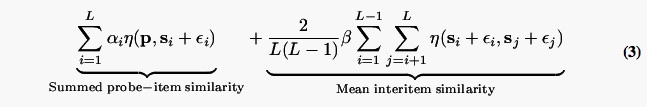
exceeds a threshold value, C. If β = 0 the model reduces to a close variant of Nosofsky's GCM model. If β < 0 a given lure will be more tempting when s₁ and s₂ are widely separated; conversely, if β > 0 a lure will be less tempting when s₁ and s₂ are widely separated.

The α and ε terms in Equation 3 determine the rate of forgetting. For the most recent item,α = 1, but for earlier items α is allowed to take on smaller values. In simulating memory for a list comprising just two stimuli, a single α parameter would determine the contribution of the older item to the summed similarity calculation. Forgetting is also modeled by allowing the variance-covariance matrix of ε to change as a function of stimulus recency. Kahana and Sekuler (2002) fit NEMO to data from lists of four items that varied along three relevant dimensions. The number of items and critical dimensions meant that a full estimation of the variance-covariance matrices for each serial position would have required estimating 24 parameters. Kahana and Sekuler therefore assumed that the covariances were zero and that the noise was fixed across serial position. In the present application to stimuli that vary along just a single critical dimension we consider the consequences of allowing the variance to change across serial position. This entails estimation of separate variance parameters for each serial position.

In the next section we consider the consequences of replacing the exponential similarity-distance function with a binary function in which similarity falls from 1 to 0 when the distance exceeds a critical threshold, (this relation is characterized by a Heavi-side function). Our motivation for considering such a binary relation between similarity and distance comes from Zhou et al.'s (2004) report that a signal detection model in which only the nearest item contributes to the recognition decision provided a reasonably good qualitative account of the mnemometric functions obtained using the roving-probe technique.¹ In comparing these two variants of NEMO we hope to determine whether an exponential or a binary summed-similarity model provides a better account of observers' visual recognition memory performance.

Fitting NEMO to mnemometric functions

We fit four different versions of NEMO to each subject's mnemometric functions by finding the parameters' values that minimized the root-mean-squared-difference (RMSD) between observed and predicted values.² The four versions represent factorial combinations of a) whether interstimulus similarity was or was not allowed to influence the response, and b) whether similarity fell exponentially with physical distance, or whether similarity was forced to be binary, falling from 1 to 0, when the probe-item distance exceeded some critical threshold. (As mentioned earlier, this binary relation is characterized by a Heaviside function). We label these four variants NEMO_βE, NEMO_βH, NEMO_E, and NEMO_H, as defined in Table 1.

Table 1.

Factorial arrangement of the four variants of NEMO fit to experimental data. In model designations, the subscripts E and H denote Exponential and Heaviside similarity-distance functions, respectively; the subscript β denotes the inclusion of an interitem similarity term.

Interstimulus similarity	Similarity-distance function
	exponential	Heaviside
yes	NEMOβE	NEMOβH
no	NEMOE	NEMOH

Because they posses an additional free parameter (β) NEMO_βE and NEMO_βH have an inherent advantage over NEMO_E and NEMO_H. To compare all four models on a more equal footing we computed Schwarz's (1978) Bayesian Information Criterion (BIC) for each model and subject. Under the simplifying assumption of normally distributed error terms, BIC is simply:

$$\mathrm{BIC}=k\ln \left(n\right)+n\ln \left(\frac{\mathit{RSS}}{n}\right)$$ (4)

where k is the number of free parameters, n is the number of observations, and RSS is the residual sum of squares. Better fitting models will have lower BIC values.

The left column of Figure 3 shows the difference between observed and predicted values for the fits of NEMO_βE and NEMO_E to the average subject data; the middle and right columns show fits to two representative subjects. Later we present formal analyses of each model's fit to each of the ten individual subjects. Figure 4 shows the differences between observed and predicted values for the fits of NEMO_βH and NEMO_H.

Figure 3.

Difference between predicted and observed mnemometric functions for exponential variants of NEMO with and without an adjustment for interstimulus similarity (i.e., NEMO_βE solid lines, and NEMO_E, dashed lines). Residuals in the lefthand column are based on averaged data, and those in the middle and righthand rows are based on individual subjects' data. The normalized spatial frequencies of s₁ and s₂ are indicated by gray bars. The panels in the upper two rows show data from the near conditions (|s₁ – s₂| = 2 JNDs); the panels in the lower two rows show data for the far conditions (|s₁ – s₂| = 8 JNDs).

Figure 4.

Difference between predicted and observed mnemometric functions for the Heaviside variants of NEMO with and without an adjustment for interstimulus similarity (i.e., NEMO_βH and NEMO_H). Residuals in the lefthand column are based on averaged data, and those in the middle and righthand rows are based on individual subjects' data. The normalized spatial frequencies of s₁ and s₂ are indicated by gray bars. The panels in the upper two rows show data from the near conditions (|s₁ – s₂| = 2 JNDs); the panels in the lower two rows show data for the far conditions (|s₁ – s₂| = 8 JNDs).

Inspection of these graphs shows that NEMO_βE (exponential, interstimulus similarity) provided the best fit to the average data (RMSD = 0.070, BIC =−635). The other models generated RMSDs ranging from 0.087 to 0.089 and BIC values ranging from −534 to −551. Whereas the inclusion of interstimulus similarity substantially improved the fit of the exponential summed-similarity models, it had little effect on the fit of the Heaviside models (see Figure 4).

Figures 3 and 4 also reveal systematic deviations between model and data for all four NEMO variants. In the near condition, the probability of making a yes response drops too slowly as the probe moves away from s₁ and s₂; this is observed in the peaks around JND =4 and JND =12 in panels a and b. In the far condition, there appears to be some systematic bias in the data that is not captured by the model. Although the residuals are much larger in the individual subject fits, one can seem many of the same trends as are present in the model fits to the average data.

Separately fitting the four NEMO variants to each of the ten subjects' data yielded a distribution of best-fitting parameter values across subjects. This analysis allowed us to generate between-subject confidence intervals for each of the parameter values and thereby assess the variation in model parameters across subjects. Table 2 reports the mean and standard error of the best-fitting parameter values for each of the four NEMO variants for the individual data.

Table 2.

Best-fitting parameter values for NEMO's fits to results

	NEMOβE		NEMOβH		NEMOE		NEMOH
Parameter	Mean	SEM	Mean	SEM	Mean	SEM	Mean	SEM
σ 1	2.109	0.166	2.346	0.200	2.299	0.239	2.364	0.218
σ 2	1.459	0.115	1.507	0.103	1.524	0.085	1.503	0.104
α	0.908	0.043	0.976	0.016	0.973	0.028	0.986	0.012
β	−0.755	0.117	−0.949	0.159
τ	0.688	0.051			0.898	0.038
Δ			1.897	0.099			1.773	0.075
Criterion	0.276	0.020	0.357	0.062	0.229	0.012	0.314	0.073
RMSD	0.113	0.005	0.121	0.005	0.129	0.005	0.125	0.005

By fitting all four model variants to individual subjects, we can quantitatively assess the differences in the BIC goodness of fit statistic for the candidate models. Table 3 shows the BIC values obtained for each subject and model. As can be seen, NEMO_βE achieves the smallest BIC in eight out of the ten subjects. The advantage of NEMO_βE over the other models proved significant (p < 0.05 by a permutation test, corrected for multiple comparisons). The other model comparisons did not attain statistical significance.

Table 3.

Values of the Bayesian Information Criterion (BIC) for each subject and model.

Subject	NEMOβE	NEMOβH	NEMOE	NEMOH
1	−460.138	−408.299	−395.327	−398.468
2	−448.709	−429.838	−457.024	−435.387
3	−428.123	−419.197	−418.838	−424.400
4	−424.155	−395.422	−411.456	−403.301
5	−505.869	−485.721	−455.823	−473.885
6	−468.497	−453.988	−465.594	−458.012
7	−494.123	−480.834	−467.319	−484.200
8	−457.325	−450.624	−434.903	−447.940
9	−426.251	−422.282	−422.250	−427.311
10	−493.830	−442.971	−403.944	−420.087

NEMO_βE's fit indicated that interstimulus similarity moderated the effect of summed-similarity on decisions. This phenomenon is seen in the significantly negative value of the β parameter (−0.76 ± 0.12), indicating that subjects are less likely to say yes when interstimulus similarity is high than when it is low. This extends previous findings of Kahana and Sekuler (2002) and Nosofsky and Kantner (2006) to an experimental paradigm in which only a single stimulus dimension (either horizontal or vertical frequency) varied.

NEMO has two mechanisms that enable it to fit the observed recency effects. First, NEMO can adopt different values for the standard deviation of ε for s₁ (denoted σ₁) and for s₂ (denoted σ₂). In fitting our data, NEMO consistently chose a smaller standard deviation for the memorial noise of the more recent stimulus (see Table 2). Borrowing from the literature on global matching models of recognition memory (Murdock & Lamon, 1988; Murdock & Kahana, 1993b), we also allow NEMO to differentially weight the contribution of s₁ and s₂ in the summed similarity calculation (this is done via the models' parameter). This increased weighting of recently experienced items may be viewed either as a decay process or as a mechanism of strategic control. In the latter interpretation, subjects may focus their memory comparison on more recently presented information, downweighting the signals from older traces. In fitting our data, NEMO consistently chose to assign a greater weight to s₂ than to s₁ (see Table 2). One could easily imagine that the model would pick one of these two mechanisms over the other, at least for individual subjects. Yet, both mechanisms appeared to play a role in accounting for the observed serial position effects. Given that the older stimulus is encoded with greater noise it would be rational to assign it less weight in the summed similarity computation.

Three factors conspire to determine how the proximal and distal stimuli (i.e., stimuli that were nearer to the probe on the spatial frequency dimension, or further from the probe on that dimension) contribute to the overall summed-similarity calculation: 1) the form of the similarity-distance function as defined in Eq. 2; 2) the noise added to the stored stimulus representations; and 3) the differential weighting of more and less recent items, as determined by α. When p's spatial frequency is close to that of both s₁ and s₂, the ratio of the summed-similarity contributions of proximal and distal items should approach one. However, when p's spatial frequency is much nearer to one of the studied items, the proximal items contribution to summed similarity will be far greater than that of the distal item. Figure 5 shows how the ratio of the proximal and distal items' contributions to summed similarity changes as a function of p's spatial frequency in each of the four experimental conditions. Here one can see that the relative contribution of the proximal item to summed similarity in comparison to that of the distal item is substantially higher in the far condition (panels c and d) than in the near condition (panels a and b).

Figure 5.

Relative contributions of proximal and distal items to summed similarity. Each panel shows p's similarity to the proximal study item divided by p's similarity to the distal study item as a function of probe position for one of the experimental conditions. The normalized spatial frequencies of s₁ and s₂ are indicated by gray bars. The upper panels show data from the near conditions; the lower panels show data for the far conditions. The panels on the left show data from the conditions in which s₁ had the lower spatial frequency of the two study items; the panels on the right show data from the conditions in which s₁ had the higher spatial frequency. The dashed line highlights the region of each curve where proximal and distal items contribute similarly to summed similarity. The values used are the mean over 5000 repetitions of NEMO_βE using the parameters given in Table 2.

We next consider what happens when we replace the exponential similarity-distance function used in NEMO_βE with a Heaviside (step) function in NEMO_βH. Note first that even with the Heaviside function, NEMO chose a significantly negative value for the β parameter, indicating that when interstimulus similarity is low, subjects are more likely to say yes when the probe is similar to one of the studied items. Although takes on a value smaller than the distance between the two studied items, even in the near condition, the model still takes on a significantly negative value for β. This means that interstimulus similarity matters despite the fact that, on average, interstimulus similarity will be zero when using the Heaviside function. This seems less mysterious when one considers that noise in the coding of s₁ and s₂ will occasionally make the distance between the studied items less than Δ, and therefore interstimulus similarity will be 1 on a portion of the trials.

Our final manipulation was to eliminate the β parameter, yielding the models designated NEMO_E and NEMO_H. The effect of this manipulation can be seen in Figure 3 and Figure 4's plots of residuals (that is, differences between predicted and observed mnemometric functions). In each panel, residuals associated with a model that includes β are shown as a solid line, and residuals associated with a model from which β has been eliminated are shown as a dotted line. In Figure 3, which presents results for the two exponential variants, NEMO_βE and NEMO_E, differences between residuals with and without β are more pronounced than the corresponding differences in Figure 4, which presents results for the model's two Heaviside variants, NEMO _βH and NEMO_H. These comparisons show clearly that the presence of β has a greater effect on the exponential models than on the Heaviside models.

Discussion

Summed-similarity models provide a major current framework for thinking about recognition and classification of stimuli whose similarity relations vary along measurable dimensions (e.g., Estes, 1994; Nosofsky, 1991; Brockdorff & Lamberts, 2000). An important contribution of these models has been in their ability to describe variation in false alarm rates as a function of the distance between a lure and the studied items (see also, Hintzman, 1988).

Extending the summed-similarity analysis to account for data on individual lists, Kahana and Sekuler (2002) found that summed-similarity models mispredicted subjects' performance on lists with very high or very low interstimulus similarity. They also found that when lists were homogeneous, subjects committed fewer false alarms to similar lures. These findings, which were obtained using sinusoidal gratings as stimuli, were extended by Nosofsky and Kantner (2006) to Munsell color stimuli.

The present experiment examined the role of interstimulus similarity in predicting subjects' false alarms to lures varying systematically in their similarity to a list of two previously studied items. This parametric manipulation of the lures' perceptual coordinates reveals a functional relation between subjects' false-alarm rate and the lure's similarity to the studied items. Zhou et al. (2004) referred to this relation as a mnemometric function, and showed that a simple signal-detection model could explain its basic form.

In the present study, we measured individual subjects' mnemometric functions for lists comprising two gratings that were separated by either 2 or 8 JNDs. Before testing memory, we measured individual subjects' discrimination thresholds, and used those thresholds to scale or tailor stimuli for each subject. Armed with a substantial dataset for recognition memory, we fit four variants of NEMO to individual subjects' mnemometric functions. The four models differed along two dimensions: a) whether they used interstimulus similarity to adjust subjects' criteria on a trialwise basis, and b) whether they used an exponential or a Heaviside function to map perceptual distance (in JND units) onto psychological similarity. The study by Zhou et al. (2004) motivated us to evaluate the form of the similarity-distance function, because the version of NEMO that assumes a Heaviside function is quite similar to the signal-detection framework presented in that paper. Individual-subject fits demonstrated a clear superiority for Kahana and Sekuler's NEMO_βE model, which uses an exponential transformation of perceptual distance, and uses interitem similarity to adjust the decision criterion (Nosofsky & Kantner, 2006). Note that despite NEMO_βE's clear superiority, each of the model variants does a respectable job of fitting the mnemometric functions. This fact serves as a reminder that, as Pitt and Myung (2002) and others have cautioned, even a seemingly good fit can be bad.

We should note that NEMO includes some implicit assumptions that need to be tested explicitly. First, as presently formulated, the model treats each trial as encapsulated, with no intrusion or bleed through from any preceding trial. Put another way, Equation 3 implies that the information used for each recognition decision is written on a blank slate, with memory being reset after each trial (c.f. Murdock & Kahana, 1993; Howard & Kahana, 2002). If this assumption were correct, recognition memory measured in this paradigm for grating stimuli would differ from memory for other classes of stimuli, including letters and words, which show strong inter-list interference effects (e.g., Monsell, 1978; Donnelly, 1988; Bennett, 1975). Moreover, with a different paradigm, visual search experiments have demonstrated bleed through from previous trials for features such as color (Huang, Holcombe, & Pashler, 2004) and, most directly relevant to our experiment, the spatial frequency of stimuli (Maljkovic & Nakayama, 1994). NEMO could be easily augmented to account for inter-list interference effects, if needed to accommodate results from extensions of experiments like the one we report here. Briefly, if recognition judgments on the n^th trial were shown to be influenced by study items on the previous trial, NEMO could be augmented by an additional term that represents summed similarity between p on the n^th trial and study items on the (n − 1)^th trial. If the proportion of inter-trial intrusions were modest, the term for inter-trial summed-similarity would be weighted substantially less than its intra-trial counterpart.

Models of contextual drift (e.g., Dennis & Humphreys, 2001; Howard & Kahana, 2002; Mensink & Raaijmakers, 1988; Murdock, 1997) offer a more sophisticated approach to the problem of interlist interference and contextually-focused retrieval. Rather than down-weighting the contribution of older memories to summed similarity, as we have done in NEMO, contextual drift models assume that each memory is tagged with a contextual representation that changes slowly over time. This vector representation of context, sometimes referred to as temporal context, integrates the patterns of brain states over time, with more recent states weighted more heavily than older states (see Howard & Kahana, 2002 for details). Within this framework, a recognition test cue is a vector of attribute values whose elements include both the attributes representing the test item itself and the attributes representing the state of temporal context at the time of test (cf. Neath, 1993). This composite test cue, representing both content and context information, is used to retrieve similar traces stored in memory. The recognition decision is then based on the similarity of this retrieved information with the test cue itself (Dennis & Humphreys, 2001; Schwartz, Howard, Jing, & Kahana, 2005). Although context based models have previously been applied primarily to data on verbal memory, it is possible to incorporate their contextual drift and contextual retrieval mechanisms into summed-perceptual-similarity models, such as NEMO.

The second assumption deserving of further study is the mechanism behind inter-item similarity's influence on recognition. In NEMO, this influence is represented by the parameter β (see Equation 3). Fits of the model have produced consistently negative values for β, which is consistent with the assumption that inter-similarity leads to an adaptive shift in the subject's criterion (Kahana & Sekuler, 2002; Nosofsky & Kantner, 2006). When study items are highly similar to one another, the associated negative β seems to increase the effective conservatism of the subject's criterion for responding yes. Hence, the negative β affords some protection against false positives. This interpretation, which locates β's role at a decision making stage, seems a reasonable hypothesis, but one that future research might examine. Several physiological and behavioral studies hint at an alternative worth considering, namely that β is mediated by a change in the sensitivity or noise of early visual mechanisms in cortical processing, well before the decision making stage. For example, Spitzer, Desimone, and Moran (1988) showed that the difficulty level of a visual discrimination task altered neuronal responses in visual area V4 of cerebral cortex. Presumably, a more difficult task makes for increased attentional demands, which increase the strength and selectivity of neuronal responses (see also McAdams & Maunsell, 1999; Reynolds & Desimone, 2003; Boynton, 2005). It would be useful, therefore, to determine whether, in recognition memory, inter-item similarity has an analogous effect, altering the the noise or sensitivity of visual mechanisms responsible for encoding study items.

References

- Ashby FG, Maddox WT. Stimulus categorization. In: Marley AAJ, editor. Choice, decision, and measurement: Essays in honor of R. Duncan Luce. Lawrence Erlbaum and Associates; Mahwah, NJ: 1998. pp. 251–301. [Google Scholar]
- Bennett RW. Proactive interference in short-term memory: Fundamental forgetting processes. Journal of Verbal Learning and Verbal Behavior. 1975;14:573–584. [Google Scholar]
- Boynton GM. Attention and visual perception. Current Opinion in Neurobiology. 2005;15:465–469. doi: 10.1016/j.conb.2005.06.009. [DOI] [PubMed] [Google Scholar]
- Brainard DH. The psychophysics toolbox. Spatial Vision. 1997;10:443–446. [PubMed] [Google Scholar]
- Brockdorff N, Lamberts K. A feature-sampling account of the time course of old-new recognition judgments. Journal of Experimental Psychology: Learning, Memory, and Cognition. 2000;26:77–102. doi: 10.1037//0278-7393.26.1.77. [DOI] [PubMed] [Google Scholar]
- Chater N, Vitanyi PMB. The generalized universal law of generalization. Journal of Mathematical Psychology. 2003;47:346–369. [Google Scholar]
- Clark SE, Gronlund SD. Global matching models of recognition memory: How the models match the data. Psychonomic Bulletin and Review. 1996;3:37–60. doi: 10.3758/BF03210740. [DOI] [PubMed] [Google Scholar]
- Della-Maggiore V, Sekuler AB, Grady CL, Bennett PJ, Sekuler R, McIntosh AR. Corticolimbic interactions associated with performance on a short-term memory task are modified by age. Journal of Neuroscience. 2000;20(22):8410–6. doi: 10.1523/JNEUROSCI.20-22-08410.2000. [DOI] [PMC free article] [PubMed] [Google Scholar]
- Dennis S, Humphreys MS. A context noise model of episodic word recognition. Psychological Review. 2001;108:452–478. doi: 10.1037/0033-295x.108.2.452. [DOI] [PubMed] [Google Scholar]
- Donnelly RE. Priming effects in successive episodic tests. Journal of Experimental Psychology: Learning, Memory, and Cognition. 1988;14:256–265. [Google Scholar]
- Ennis DM, Palen J, Mullen K. A multidimensional stochastic theory of similarity. Journal of Mathematical Psychology. 1988;32:449–465. [Google Scholar]
- Estes WK. Classification and cognition. Oxford University Press; Oxford, U. K.: 1994. [Google Scholar]
- Hintzman DL. Judgments of frequency and recognition memory in multiple-trace memory model. Psychological Review. 1988;95:528–551. [Google Scholar]
- Howard MW, Kahana MJ. A distributed representation of temporal context. Journal of Mathematical Psychology. 2002;46:269–299. [Google Scholar]
- Huang L, Holcombe AO, Pashler H. Repetition priming in visual search: episodic retrieval, not feature priming. Memory & Cognition. 2004;32:12–20. doi: 10.3758/bf03195816. [DOI] [PubMed] [Google Scholar]
- Humphreys MS, Pike R, Bain JD, Tehan G. Global matching: A comparison of the SAM, Minerva II, Matrix, and TODAM models. Journal of Mathematical Psychology. 1989;33:36–67. [Google Scholar]
- Hwang G, Jacobs J, Geller A, Danker J, Sekuler R, Kahana MJ. EEG correlates of subvocal rehearsal in working memory. Behavioral and Brain Functions. 2005;1:20. doi: 10.1186/1744-9081-1-20. [DOI] [PMC free article] [PubMed] [Google Scholar]
- Kahana MJ, Bennett PJ. Classification and perceived similarity of compound gratings that differ in relative spatial phase. Perception & Psychophysics. 1994;55:642–656. doi: 10.3758/bf03211679. [DOI] [PubMed] [Google Scholar]
- Kahana MJ, Rizzuto DS, Schneider A. An analysis of the recognition-recall relation in four distributed memory models. Journal of Experimental Psychology: Learning, Memory, and Cognition. 2005;31:933–953. doi: 10.1037/0278-7393.31.5.933. [DOI] [PubMed] [Google Scholar]
- Kahana MJ, Sekuler R. Recognizing spatial patterns: A noisy exemplar approach. Vision Research. 2002;42:2177–2192. doi: 10.1016/s0042-6989(02)00118-9. [DOI] [PubMed] [Google Scholar]
- Lamberts K, Brockdorff N, Heit E. Feature-sampling and random-walk models of individual-stimulus recognition. Journal of Experimental Psychology: General. 2003;132:351–378. doi: 10.1037/0096-3445.132.3.351. [DOI] [PubMed] [Google Scholar]
- Maddox WT. On the dangers of averaging across observers when comparing decision bound models and generalized context models of categorization. Perception & Psychophysics. 1999;61(2):354–374. doi: 10.3758/bf03206893. [DOI] [PubMed] [Google Scholar]
- Maddox WT, Ashby FG. Perceptual separability, decisional separability, and the identification-speeded classification relationship. Journal of Experimental Psychology: Human Perception and Performance. 1996;22:795–817. doi: 10.1037//0096-1523.22.4.795. [DOI] [PubMed] [Google Scholar]
- Maljkovic V, Nakayama K. Priming of pop-out: I. role of features. Memory & Cognition. 1994;22:657–672. doi: 10.3758/bf03209251. [DOI] [PubMed] [Google Scholar]
- McAdams CJ, Maunsell JH. Effects of attention on the reliability of individual neurons in monkey visual cortex. Neuron. 1999;23:765–773. doi: 10.1016/s0896-6273(01)80034-9. [DOI] [PubMed] [Google Scholar]
- McKinley SC, Nosofsky RM. Selective attention and the formation of linear decision boundaries. Journal of Experiment Psychology: Human Perception and Performance. 1996;22:294–317. doi: 10.1037//0096-1523.22.2.294. [DOI] [PubMed] [Google Scholar]
- Mensink G-JM, Raaijmakers JGW. A model for interference and forgetting. Psychological Review. 1988;95:434–455. [Google Scholar]
- Monsell S. Recency, immediate recognition memory, and reaction time. Cognitive Psychology. 1978;10:465–501. [Google Scholar]
- Morgan MJ, Watamaniuk SN, McKee SP. The use of an implicit standard for measuring discrimination thresholds. Vision Research. 2000;40(17):2341–2349. doi: 10.1016/s0042-6989(00)00093-6. [DOI] [PubMed] [Google Scholar]
- Murdock BB. Context and mediators in a theory of distributed associative memory (TODAM2) Psychological Review. 1997;104:839–862. [Google Scholar]
- Murdock BB, Kahana MJ. Analysis of the list strength effect. Journal of Experimental Psychology: Learning, Memory and Cognition. 1993a;19:689–697. doi: 10.1037/0278-7393.19.6.1445. [DOI] [PubMed] [Google Scholar]
- Murdock BB, Kahana MJ. List-strength and list-length effects: Reply to Shiffrin, Ratcliff, Murnane, and Nobel. Journal of Experimental Psychology: Learning, Memory and Cognition. 1993b;19:1450–1453. doi: 10.1037/0278-7393.19.6.1445. [DOI] [PubMed] [Google Scholar]
- Murdock BB, Lamon M. The replacement effect: Repeating some items while replacing others. Memory & Cognition. 1988;16:91–101. doi: 10.3758/bf03213476. [DOI] [PubMed] [Google Scholar]
- Neath I. Distinctiveness and serial position effects in recognition. Memory & Cognition. 1993;21:689–698. doi: 10.3758/bf03197199. [DOI] [PubMed] [Google Scholar]
- Nosofsky RM. Choice, similarity, and the context theory of classification. Journal of Experimental Psychology: Learning, Memory and Cognition. 1984;10(1):104–114. doi: 10.1037//0278-7393.10.1.104. [DOI] [PubMed] [Google Scholar]
- Nosofsky RM. Attention, similarity, and the identification-categorization relationship. Journal of Experimental Psychology: General. 1986;115:39–57. doi: 10.1037//0096-3445.115.1.39. [DOI] [PubMed] [Google Scholar]
- Nosofsky RM. Tests of an exemplar model for relating perceptual classification and recognition memory. Journal of Experimental Psychology: Human Perception and Performance. 1991;17(1):3–27. doi: 10.1037//0096-1523.17.1.3. [DOI] [PubMed] [Google Scholar]
- Nosofsky RM. Exemplar-based approach to relating categorization, identification, and recognition. In: Ashby FG, editor. Multidimensional models of perception and cognition. Lawrence Erlbaum and Associates; Hillsdale, New Jersey: 1992. pp. 363–394. [Google Scholar]
- Nosofsky RM, Kantner J. Exemplar similarity, study list homogeneity, and short-term perceptual recognition. Memory and Cognition. 2006;34(1):112–124. doi: 10.3758/bf03193391. [DOI] [PubMed] [Google Scholar]
- Pelli DG. The videotoolbox software for visual psychophysics: Transforming numbers into movies. Spatial Vision. 1997;10:437–442. [PubMed] [Google Scholar]
- Pelli DG, Robson JG, Wilkins AJ. Designing a new letter chart for measuring contrast sensitivity. Clinical Vision Sciences. 1988;2:187–199. [Google Scholar]
- Petzold P, Haubensak G. Short-term and long-term frames of reference in category judgments: A multiple-standards model. In: Kaernbach C, Schroger E, editors. Psychophysics beyond sensation: Laws and invariants of human cognition. Erlbaum; Mahwah, N J: 2004. pp. 45–68. [Google Scholar]
- Pitt MA, Myung IJ. When a good fit can be bad. Trends in Cognitive Science. 2002;6:421–425. doi: 10.1016/s1364-6613(02)01964-2. [DOI] [PubMed] [Google Scholar]
- Reynolds JH, Desimone R. Interacting roles of attention and visual salience in v4. Neuron. 2003;37:853–863. doi: 10.1016/s0896-6273(03)00097-7. [DOI] [PubMed] [Google Scholar]
- Rizzuto DS, Kahana MJ. An autoassociative neural network model of paired associate learning. Neural Computation. 2001;13:2075–2092. doi: 10.1162/089976601750399317. [DOI] [PubMed] [Google Scholar]
- Schwartz G, Howard MW, Jing B, Kahana MJ. Shadows of the past: Temporal retrieval effects in recognition memory. Psychological Science. 2005;16:898–904. doi: 10.1111/j.1467-9280.2005.01634.x. [DOI] [PMC free article] [PubMed] [Google Scholar]
- Schwarz G. Estimating the dimension of a model. Annals of Statistics. 1978;6(2):461–464. [Google Scholar]
- Sekuler R, Kahana MJ, McLaughlin C, Golomb J, Wingfield A. Preservation of episodic visual recognition memory in aging. Experimental Aging Research. 2005;31:1–13. doi: 10.1080/03610730590882800. [DOI] [PubMed] [Google Scholar]
- Shepard RN. Toward a universal law of generalization for psychological science. Science. 1987;237:1317–1323. doi: 10.1126/science.3629243. [DOI] [PubMed] [Google Scholar]
- Spitzer H, Desimone R, Moran J. Increased attention enhances both behavioral and neuronal performance. Science. 1988;240:338–340. doi: 10.1126/science.3353728. [DOI] [PubMed] [Google Scholar]
- Sternberg S. High-speed scanning in human memory. Science. 1966;153:652–654. doi: 10.1126/science.153.3736.652. [DOI] [PubMed] [Google Scholar]
- Sternberg S. Memory scanning: New findings and current controversies. Quarterly Journal of Experimental Psychology. 1975;27:1–32. [Google Scholar]
- Treisman M, Williams TC. A theory of criterion setting with an application to sequential dependencies. Psychological Review. 1984;91:68–111. [Google Scholar]
- Wetherill GB, Levitt H. Sequential estimation of points on a psychometric function. British Journal of Methematical and Statistical Psychology. 1965;18(1):1–10. doi: 10.1111/j.2044-8317.1965.tb00689.x. [DOI] [PubMed] [Google Scholar]
- Zhou F, Kahana MJ, Sekuler R. Short-term episodic memory for visual textures: A roving probe gathers some memory. Psychological Science. 2004;15:112–118. doi: 10.1111/j.0963-7214.2004.01502007.x. [DOI] [PubMed] [Google Scholar]