Representation of spatial frequency and orientation in the visual cortex

Abstract

Knowledge of the response of the primary visual cortex to the various spatial frequencies and orientations in the visual scene should help us understand the principles by which the brain recognizes patterns. Current information about the cortical layout of spatial frequency response is still incomplete because of difficulties in recording and interpreting adequate data. Here, we report results from a study of the cat primary visual cortex in which we employed a new image-analysis method that allows improved separation of signal from noise and that we used to examine the neurooptical response of the primary visual cortex to drifting sine gratings over a range of orientations and spatial frequencies. We found that (i) the optical responses to all orientations and spatial frequencies were well approximated by weighted sums of only two pairs of basis pictures, one pair for orientation and a different pair for spatial frequency; (ii) the weightings of the two pictures in each pair were approximately in quadrature (1/4 cycle apart); and (iii) our spatial frequency data revealed a cortical map that continuously assigns different optimal spatial frequency responses to different cortical locations over the entire spatial frequency range.

The primary visual cortex has the apparatus to sort out the ingredients needed to perform a variety of visual functions. An important example is that of perceptual invariance: the ability to recognize a pattern as itself after its size or orientation have been changed. It has long been known from single-cell recordings that cortical neurons are selective for both orientation and spatial frequency. Hubel and Wiesel (1, 2) first reported the systematic arrangement of neurons with similar orientation preference, and subsequent optical imaging studies (3, 4) have reported consistent results about the cortical layout of orientation-selective cells. Studies of the primate visual cortex led DeValois and DeValois (5) to propose a polar architecture of spatial frequency selectivity (see also ref. 6) tied to the cytochrome oxidase blobs. The issue has been re-examined in recent optical imaging work (7, 8), but no consensus has been reached.

Here, we address these issues with two new technical developments. The first is the use of the recently published method of indicator functions (9). Our second technical development is the extraction of a small basis set of images from a collection of optical response pictures taken under a variety of stimulus conditions. To this end, we ask if there is a small set of images that could serve as a set of coordinates in the sense that, added together in appropriately weighted combinations, they can be used to reconstruct the response images obtained from the various stimuli. In the present study, we find that two basis pictures suffice essentially to reconstruct the orientation response when spatial frequencies are pooled, and another set of two pictures reconstructs the spatial frequency response when orientations are pooled. This approach yields a compact quantitative description of the optical response of cortex to both orientation and spatial frequency. Our method confirms the consensus of previous studies (3, 4) regarding cortical response to stimulus orientation and does so without recourse to the implicit assumption that lies in the method of vector summation. However, our method directly applies also to the response of primary visual cortex to various spatial frequencies, where it provides an additional insight.

METHODS

Surgery and Imaging.

The experiments were carried out on six adult (2–5 kg) cats (Felis domestica). Anesthesia was induced with i.m. injections of Xylazine [Rompun (Miles), 2 mg⋅kg⁻¹] and Ketamine [Ketaset (Fort Dodge Laboratories, Fort Dodge, IA), 10 mg⋅kg⁻¹] and later was maintained with i.v. infusion of Pentothal (Astra, Westborough, MA) (1–3 mg⋅kg⁻¹⋅hr⁻¹). Muscular paralysis was induced by i.v. infusion of Pancuronium bromide (Abbott) (1.3 mg⋅kg⁻¹⋅hr⁻¹). The state of anesthesia was monitored and maintained carefully in accordance with the National Institutes of Health guidelines. The animals were respired mechanically and the end-expiratory concentration of CO₂ was kept at 3.5–4%. Blood pressure, electroencephalogram, electrocardiogram, and core body temperature were monitored and maintained within normal physiological ranges. The eyes were protected with gas-permeable, hard contact lenses, and corrective lenses were used to focus the eyes at the distance at which the cathode ray tube monitor was placed, usually 57 cm. Each eye viewed the stimuli through a 3-mm artificial pupil, and translucent shutters permitted presentation of either a pattern or diffuse illumination to either eye. A craniotomy and durotomy exposed a region of V1 corresponding to 2–8° eccentricity in the visuotopic representation. A cylindrical, stainless steel, glass-topped chamber was attached to the skull with screws and plumbers epoxy (Propoxy 20, Hercules, Passaic, NJ), and was filled with inert silicone oil. The cortex was illuminated uniformly with 600 nm light and imaged through a tandem-lens configuration (10) by using a cooled 12-bit charge-coupled device (PXL, Photometrics, Tucson, AZ, 536 × 389 pixels) that was synchronized to the cardiac and respiratory cycles (4).

Visual Stimuli.

All stimuli consisted of drifting sinusoidal gratings of spatial frequencies between 0.02 and 2.28 cycles per degree, each presented at four orientations (0°, 45°, 90°, and 135°) in a pseudo-random sequence. The six spatial frequencies we used were 0.07, 0.14, 0.28, 0.57, 1.14, and 2.28 cycles per degree for the data in Fig. 1 Left and 0.033, 0.067, 0.135, 0.27, 0.54, and 1.08 cycles per degree for the data in Fig. 1 Right. The gratings drifted at a temporal frequency of 2 Hz and were of 100% contrast. Each stimulus was repeated 20 times. The cathode ray tube subtended 20–28° of visual angle.

Figure 1.

(Left and Right) Data from two anesthetized cats. (a) Exposed visual cortex; the region used for detailed analysis is outlined. (b and c) The two “basis” pictures ψ_n(x) that generate the averaged orientation optical responses. (d) Weighting coefficient curves, a_n(θ), which weight basis pictures b and c to yield the orientation response at a given angle. (e) Locus of orientation optical response “vectors” in two-dimensional section through pixel space. (f) Pattern of orientation pinwheels; color indicates preferred angle in degrees. (g) Strength of “orthogonal orientation difference response” vs. spatial frequency; the two curves are vertical–horizontal (solid) and diagonal (dashed) differences. Logarithmic cycles-per-degree scale also appears in j below. (h and i) The two basis pictures ψ_n(x) that generate the averaged spatial frequency response. (j) Weighting curves, a_n(ν), which weight h and i to yield optical spatial frequency response. (k) Locus of spatial frequency optical response vectors in two-dimensional section through pixel space. (l) Patterns of spatial frequency pinwheels; color indicates preferred spatial frequency in cycles per degree.

Image Analysis.

We briefly describe the mathematical procedures used in the data analysis. The discussion is phrased in terms of orientations, but exactly analogous procedures were used for the spatial frequency data.

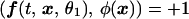
Indicator functions. We used indicator functions, which constitute a recent improvement in the extraction of weak image changes (9). This method exploits conditional averaging along with the fact that an orderly picture exhibits substantial interpixel correlations, which are absent from disorderly noise. As an initial step in the data processing, from each frame recorded after a presentation of a stimulus we subtracted the average reflectance of three response images collected just before the presentation of that stimulus. Next, we performed principal components analysis (11) on the entire data set, which typically exceeded 10,000 images, taken under all stimulus conditions. Only the first 50–100 principal components contained information related to the visual response, and a linear combination of these relevant principal components was used to construct the indicator function. As in the difference of averages method (4), the generation of indicator functions depends on a comparison of images collected during two contrasting stimulus conditions. An indicator function is a new picture generated from the raw images such that its inner product (which is proportional to correlation) with images from a particular orientation, say, θ₁, is as close as possible to +1, and its inner product with images from the contrasting orientation, say, θ₂, is as close as possible to −1. In other words, if we denote by ƒ(t, x, θ) images (with prestimulus frames subtracted) collected in response to orientation θ, where x is a pixel location and t indexes the images, then the indicator image, φ(x), is the image that best satisfies, in a variational sense, the following criteria:

where (ƒ, φ) is the spatial inner product (summed products of pixel values) of images ƒ and φ.

We performed extensive image-extraction experiments on simulated data sets in which we buried known images under sequential frames of noisy laboratory data, and we confirmed the ability of our technique to extract a quality approximation of the input image under signal-to-noise conditions in which the usual methods fail (9, 12). Under sufficiently clean signal-to-noise conditions, our method and the usual methods give similar results. Because the indicator function method depends on contrasting responses to stimuli that are similar in all respects except for the variable under investigation and because it gives similar results to differential imaging when the signal/noise ratio is large, it is convenient to think of the method as an enhanced differencing procedure.

Pairwise indicator functions.

Each of our 24 stimuli (four orientations, each at six spatial frequencies) was presented 20 times. The resulting data, for each cat, were divided into four subsets according to orientation. These four subsets were paired in all six possible pairs; then, indicator functions φ_ij(x) were found for all pairs of stimulating angles θ_i and θ_j, i ≠ j. In an exactly analogous manner, pairwise indicator functions were generated to contrast all 15 possible pairs of the six spatial frequency responses. All pairs were differenced, rather than just orthogonal pairs. This was done (i) to avoid the introduction of a possible artifact through orthogonal selection; and (ii) to follow a procedure that can be applied when spatial frequency, rather than orientation, is the variable. Although stimuli with different orientations elicit strongest responses at different locations on the cortex, the magnitude of the overall response is approximately the same for all orientations. However, the magnitude (as well as the location) differs for stimuli of different spatial frequencies because very low and very high spatial frequencies elicit little response (Fig. 1 panels g). The even-handed use of all difference pairs avoids some artifacts that arise, for example, when both strong and weak individual responses are differenced against a single “cocktail” superposition of strong and weak responses; in such differences, the weakest responses are overwritten by the negatives of the strongest contributors to the cocktail.

A second principal components analysis.

The question of “how many pictures are required to generate all pairwise average difference images or indicator images” was addressed by a second principal components analysis, this time applied to the set of pairwise images (11). More specifically, we sought basis functions or images ψ_n(x), that span the subspace of the neurooptical responses. In a least-squares sense, the optimal bases are generated by this principal components analysis.

RESULTS

We studied six adult cats and illustrate our results with data from two cats. The results from the remaining cats were consistent with these. Fig. 1 is divided into two panels that show data from the two cats. Fig. 1 panels a show a region of primary visual cortex, including blood vessels, and, within the outline, the area of detailed analysis. To explain the present technique we will first discuss its application to orientation response, and we then will apply it to the spatial frequency response.

Orientation.

Principal components analysis found two principal components or basis images, ψ_n(x), that contributed significantly to the generation of the six pairwise difference images or indicator functions. Therefore, the cortical response to any oriented stimulus may be described in terms of just these two basis pictures. Fig. 1 panels b and c are the two basis pictures, color-coded to show both positive and negative values, and which resemble the orientation columns imaged by other investigators (3, 4).

In order to find out how much each basis picture (principal component) contributes to the response at a particular stimulus orientation, we carried out the following procedure. At each stimulus orientation, θ, we “projected” (or “correlated”) each response image against each of the two basis pictures ψ₁(x) and ψ₂(x) (that is, we multiplied each pixel in a response image by the corresponding pixel in a basis picture and summed over pixels). We then averaged over response pictures at that orientation to find the corresponding two average weighting coefficients a₁(θ) and a₂(θ) of the basis picture in the orientation response at that orientation. Thus, a_n(θ) = (F(x, θ), ψ_n(x)), where F(x, θ) is the average of all images collected at orientation θ. The data points on the two smooth curves in Fig. 1 panels d show the values that these coefficients have for stimulus orientations of θ = 0°, 45°, 90°, 135°, and 180° (the data points for 0 and 180° are the same). The smooth curves have been interpolated through those points; the interpolated curves in Fig. 1 panels d and j prove insensitive to the interpolation method. As a consequence of our construction, at any orientation where one of these curves passes through zero, the spatial distribution of the optical orientation response is proportional to the complementary basis picture; at intermediate orientations, the response is the sum of the basis functions weighted by the coefficients a_n(θ).

As we noted above, two principal components or basis pictures are sufficient to represent the orientation response. The two principal components together account for 89% (cat I) and 84% (cat II) of the variance in all of the pairwise difference images. The third principal component accounts for only 6.5% (cat I) and 7% (cat II) of the variance and makes no significant difference to the conclusions below. However, both of the first two basis functions are essential for a faithful representation of the orientation response. Using either one alone completely misses the intrinsically two-dimensional nature of the response. Previous work (3, 4) has tacitly assumed this two-dimensionality; here, we provide direct evidence that the cortex is so organized.

Fig. 1 panels b and c are each constructed from a list of numerical pixel values, and they may be regarded as two vectors in a space whose dimension is equal to the number of pixels. As principal component vectors, they have the property that they are orthogonal vectors in the sense that the summed product of their pixel values is zero (their cross-correlation is zero). Together, they define a two-dimensional plane within the high-dimensional pixel space. The orientation-response images, as weighted combinations of the two basis pictures, correspond to points in that plane. Representing Fig. 1 panels b and c by horizontal and vertical vectors in the plane of Fig. 1 panels e, we use the two weighting curves a₁(θ) and a₂(θ) of Fig. 1 panels d to construct (on the plane of Fig. 1 panels e) the locus of orientation–response images represented as vectors in that plane. Thus, as the stimulus orientation sweeps clockwise through 360°, the orientation response is represented as traveling twice around the locus. The locus is circle-like, with data points almost equidistantly spaced along it; these conditions would be fulfilled exactly if the two curves of Fig. 1 panels d were exactly sine and cosine. It is the neural organization of the visual cortex that both has restricted the optical response images, conceived of as vectors in pixel space, to a two dimensional plane, and has produced the simple geometric relation in that plane shown in Fig. 1 panels e. This result is independent of the particular choice of orientations, as confirmed by other experiments.

The data we show here permit us to find the stimulus orientation that elicits the best response at each cortical location. Fig. 1 panels b and c assign to each pixel two response intensity values whose weighted sum, taken from the curves of Fig. 1 panels d, states the response amplitude for that pixel as a function of orientation angle. This information, in turn, tells us the orientation angle at which that pixel gives its maximum response. In Fig. 1 panels f, we have color-coded the best response angle at each cortical location, and we see an orderly progression with changing cortical position. The “pinwheel axles,” where all colors come together, are the locations where the response amplitudes in Fig. 1 panels b and c go through zero.

Our analysis is quite different from the commonly applied procedure of “vector summation,” which is used to extract orientation “pinwheels” from image data (3, 4) (see also ref. 13). The application of vector summation to our starting orientation responses gives a picture in good agreement with Fig. 1 panels f. We observe that, in form, the two curves in Fig. 1 panels d together bear a striking resemblance to sine and cosine; indeed, to a fair approximation where either curve crosses zero its companion achieves an extremum. This result is a consequence of the nature of the orientation response and has not been imposed by our data analysis. Vector summation assumes a priori that the cortical response conforms to a two-dimensional model in which the weighting curves are sine and cosine, so that the locus (Fig. 1 panels e) would be a circle. It is not hard to argue from the natural periodicity of grating stimuli, with increasing angle, that something qualitatively like this should occur, and that the good fit of data to maps generated by vector summation provides additional evidence for the two-dimensional model. Here, we provide direct evidence of the validity of the assumptions implicit in vector summation.

Spatial Frequency.

The same analysis procedure that we have applied to orientation can also address changes in the spatial frequency of the visual stimuli. To confirm that our data contain effects of such change, in Fig. 1 panels g, we show, at several spatial frequencies, the amplitude of the optical response in the indicator image from stimuli at right-angles. There are two curves: One shows vertical vs. horizontal stimuli, and the other shows the difference of opposite diagonal stimuli. The two experiments shown in Fig. 1 panels g, covered somewhat different spatial frequency ranges, but both included a maximum responsiveness at essentially the same spatial frequency near 0.15 cycles per degree [a reasonable maximum for cats (14)].

In the analogous manner to the analysis of orientation data, we paired the six data sets at different spatial frequencies in all 15 possible pairs and derived their 15 pairwise indicator images. A principal components analysis of those pairwise images once again yields two dominating basis pictures, which account for 74% and 63% of the variance in the 15 difference images. These spatial frequency columns, which are shown in Fig. 1 panels h and i, are fairly similar to the orientation columns of Fig. 1 panels b and c. Although it is a consequence of our analysis that the images in Fig. 1 panels h and i are mutually orthogonal to (uncorrelated with) each other, each of them is also almost orthogonal (the closest correlation is ≈0.1) to images in Fig. 1 panels b and c, and that is a consequence of cortical organization.

As we did with orientation, we calculated the weighting coefficients for the admixtures in Fig. 1 panels h and i in the optical response at each spatial frequency, and these are shown in Fig. 1 panels j. The fact that the two basis pictures, Fig. 1 panels h and i, suffice to span the averaged spatial frequency responses again implies that these responses lie in a two-dimensional plane in pixel space. Their locus in that plane is shown in Fig. 1 panels k; increasing spatial frequencies move counterclockwise on the curve. Once again, we emphasize that two basis pictures are necessary for a faithful description of the cortical response to spatial frequency. Adding a third basis function makes only a small difference in our results, in effect bending the locus of responses slightly out of the plane. On the other hand, using only one basis picture gives a severely distorted reproduction of the response.

At very low and very high spatial frequencies, the visual system is unresponsive and, as Fig. 1 panels g show, the cortical response falls off. One could hardly expect, therefore, that the curves of Fig. 1 panels j would be sinusoidal. Nonetheless, we again see that, where either curve crosses zero, its companion tends to have a nearby extremum. In fact, in the locus-plot of Fig. 1 panels k, the part of the curve defined by the four midrange data points, which spans a factor of 8 in spatial frequency, may be described as roughly an arc of a circle, and the data points (which correspond to equal logarithmic steps in stimulus magnification) cut the arc into three segments of about equal length.

The optimal spatial frequency at each pixel is color-coded in Fig. 1 panels l. Here, unlike Fig. 1 panels f, where the continuity in orientation induces a smooth change of color everywhere, the low-frequency (deep blue) and high frequency (deep red) ends of the spatial frequency range lead to discontinuities. Spatial frequency pinwheel axles appear again where the response goes through zero in Fig. 1 panels h and i. We recorded from cortical neurons in the regions that we imaged and validated the spatial frequency selectivity of the clusters our analysis here identified (A.K.P., R.M.E., B.W.K., L.S., and E.K., unpublished material).

DISCUSSION

Our data (Fig. 1 panels g) show non-zero responses over the full range of spatial frequencies used in our study. Currently, there are two contrasting views of the representation of spatial frequency in the primary visual cortex. One holds that there are two complementary cortical regions, one selective for low and the other for high spatial frequency (8, 15). The other view suggests that all spatial frequencies are separately represented, in a graded fashion, across the cortex (for example, refs. 16, 17, and 18). Tootell et al. (6) nonjudgmentally present evidence in support of both views. Based on 2-deoxyglucose data, DeValois and DeValois (5) proposed a radial arrangement of spatial frequency selectivity related to the CO blobs. Evidence from psychophysics (19) and from electrophysiology (14) indicates that all spatial frequencies are represented continuously in the cortex. Our study also supports the continuous representation view because the two-stream alternative would yield only a single significant basis picture, and the locus in Fig. 1 panels k would be reduced to a horizontal straight line. We emphasize that, like the orientation response, the spatial frequency response requires at least two dimensions for its representation. An attempt to reconstruct spatial frequency data from one basis picture, rather than two, leads to major degradation in the accuracy of the reconstruction and fundamentally changes the nature of the modeled response. The recent report of Shoham et al. (8), which supported the two-stream hypothesis, used mainly data from kittens; the difference between their observations and what we report here may reflect postnatal developmental changes in the cat visual cortex.

The major share of variance in our data is accounted for by a two-dimensional subspace, but the remaining variance still may be of significance. However, in all instances, we found the signal corresponding to the additional variance to be contaminated heavily by noise. We may speculate that other dimensions could fine tune and sharpen the curves of the orientation and spatial frequency responses.

A comment is in order concerning the mathematical structure of the cortical organization that has been shown here, in as much as mathematical structure often has proven a valuable guide to understanding neural function. The set of changes in stimulus orientation, and the set of changes in stimulus scale, may each be regarded as a one-parameter symmetry group of transformations. Our analysis has exploited the fact that a change in stimulus induces a change in an optical response image that may be regarded as a vector in a conceptual “pixel space.” Such an action of a symmetry group on vectors (if some consistency demands are fulfilled) is known as a group representation. The simplest of nontrivial group representations are two-dimensional,* which conforms to what we have presented here. To the extent that the curves in Fig. 1 panels d are sine and cosine, the locus in Fig. 1 panels e technically displays the action of a mathematically familiar two-dimensional representation of the one-parameter rotation group. In the case of stimulus rotations, this bit of group representation theory simply formalizes data manipulations to which investigators already have been led by good common sense. Some elementary arguments have been given (20) that indicate that we may indeed expect the cortex to have a layout that conforms to a two-dimensional representation of the rotation group.

In the case of scale-changes, what we should expect to find in the cortex is less evident, and the mathematical structure may be helpful for understanding function. In fact, the group of scale changes likewise has two-dimensional representations, in which the action of its elements carries a vector around the plane in a circular locus. The angle change induced by a group element is proportional to the logarithm of its scale change. In the midrange of grating sizes, we see that the same features emerge from our data analysis (Fig. 1 panels j). For the data of either cat shown in the figure, a half cycle is achieved with about a factor of 16 in scale change. Roughly speaking, an immediate physiological implication is that, if a visually centered object is presented at two scales that lie within the midrange here, equal areas of cortex (whose locations serve to index the different size scales) will be activated. This fact is also apparent from the approximately equal numbers of pixels devoted to logarithmic spatial frequency in Fig. 1 panels l. We note that Fig. 1 panels f and l together assign two colors to each pixel, which implies an assignment of both orientation and scale to each cortical location.

In a more speculative vein, we note that the primary visual cortex has sorted out the raw materials needed to perform a very important visual function. When a portrait (or the page before the reader) is rotated through a modest angle, it is immediately recognized as the same portrait. Subjectively, its sameness stands out far more than the fact of its changed orientation; this is the phenomenon of perceptual rotation invariance. If the portrait is moved away by a modest factor (two or three), again its sameness is subjectively more salient than its reduction in size; this is perceptual scale invariance. These two cases of the separation of the intrinsic features of the observed object itself from the variables of viewing condition are substantial challenges in pattern recognition, which somehow the visual cortex solves well. Our study shows that neurons that deal with these two elements of perceptual invariance are clustered in similar spatial arrangements and that the primary visual cortex represents orientation and spatial frequency in ways that are mathematically and structurally similar.

References

- 1.Hubel D, Wiesel T. J Physiol (London) 1963;165:559–568. doi: 10.1113/jphysiol.1963.sp007079. [DOI] [PMC free article] [PubMed] [Google Scholar]
- 2.Hubel D, Wiesel T. J Comp Neurol. 1974;158:267–294. doi: 10.1002/cne.901580304. [DOI] [PubMed] [Google Scholar]
- 3.Bonhoeffer T, Grinvald A. Nature (London) 1991;353:429–431. doi: 10.1038/353429a0. [DOI] [PubMed] [Google Scholar]
- 4.Blasdel G. J Neurosci. 1992;12:3115–3138. doi: 10.1523/JNEUROSCI.12-08-03115.1992. [DOI] [PMC free article] [PubMed] [Google Scholar]
- 5.DeValois R, DeValois K. Spatial Vision. Oxford Univ. Press: New York; 1988. [Google Scholar]
- 6.Tootell R, Silverman M, Hamilton S, Switkes E, DeValois R. J Neurosci. 1988;8:1610–1624. doi: 10.1523/JNEUROSCI.08-05-01610.1988. [DOI] [PMC free article] [PubMed] [Google Scholar]
- 7.O’Brien E, Prashanth A, Knight B, Kaplan E. Soc Neurosci Abstr. 1995;22:1704. [Google Scholar]
- 8.Shoham D, Hubener M, Schulze S, Grinvald A, Bonhoeffer T. Nature (London) 1997;385:529–533. doi: 10.1038/385529a0. [DOI] [PubMed] [Google Scholar]
- 9.Everson R, Knight B, Sirovich L. Biol Cybernetics. 1997;77:407–417. doi: 10.1007/s004220050400. [DOI] [PubMed] [Google Scholar]
- 10.Ratzlaff E, Grinvald A. J Neurosci Methods. 1991;36:127–137. doi: 10.1016/0165-0270(91)90038-2. [DOI] [PubMed] [Google Scholar]
- 11.Sirovich L, Everson R. Int J Supercomputing Applications. 1992;6:50–68. [Google Scholar]
- 12.Everson, R., Sirovich, L., Knight, B., Kaplan, E., O’Brien, E. & Orbach, D. (1998) Bio. Bull., in press.
- 13.Zhang J. Biol Cybernetics. 1990;63:135–142. doi: 10.1007/BF00203036. [DOI] [PubMed] [Google Scholar]
- 14.DeAngelis G, Ohzawa I, Freeman R. J Neurophysiol. 1993;69:1091–1117. doi: 10.1152/jn.1993.69.4.1091. [DOI] [PubMed] [Google Scholar]
- 15.Hübener M, Shoham D, Grinvald A, Bonhoeffer T. J Neurosci. 1997;17:9270–9284. doi: 10.1523/JNEUROSCI.17-23-09270.1997. [DOI] [PMC free article] [PubMed] [Google Scholar]
- 16.Tootell R, Silverman M, DeValois R. Science. 1981;214:813–815. doi: 10.1126/science.7292014. [DOI] [PubMed] [Google Scholar]
- 17.Prashanth A, Everson R, Kaplan E. Soc Neurosci Abstr. 1997;23:568. [Google Scholar]
- 18.Silverman M, Grosof D, DeValois R, Elfar S. Proc Natl Acad Sci USA. 1989;86:711–715. doi: 10.1073/pnas.86.2.711. [DOI] [PMC free article] [PubMed] [Google Scholar]
- 19.Campbell F, Robson J. J Physiol (London) 1968;197:551–566. doi: 10.1113/jphysiol.1968.sp008574. [DOI] [PMC free article] [PubMed] [Google Scholar]
- 20.Sirovich L, Everson R, Kaplan E, Knight B, O’Brien E, Orbach D. Physica D. 1995;96:355–366. [Google Scholar]