Self-Rated Health Trajectories and Mortality Among Older Adults

Abstract

Objectives

For this article, we evaluated whether measures of prior self-rated health (SRH) trajectories had associations with subsequent mortality that were independent of current SRH assessment and other covariates.

Methods

We used multivariable logistic regression that incorporated four waves of interview data (1993, 1995, 1998, and 2000) from the Asset and Health Dynamics Among the Oldest Old Survey in order to predict mortality during 2000–2002. We defined prior SRH trajectories for each individual based on the slope estimated from a simple linear regression of their own SRH between 1993 and 1998 and the variance around that slope. In addition to SRH reported in 2000, other covariates included in the mortality models reflected health status, health-related behaviors, and individual resources.

Results

Among the 3,129 respondents in the analytic sample, SRH in 2000 was significantly (p < .0001) associated with mortality, but the measures of prior SRH trajectories were not. Prior SRH trajectory was, however, a significant determinant of current SRH. We observed significant independent associations with mortality for age, sex, education, lung disease, and having ever smoked.

Discussion

Although measures of prior SRH trajectories did not have significant direct associations with mortality, they did have important indirect effects via their influence on current SRH.

Researchers first documented the association between self-rated health (SRH) and mortality in the early 1980s (Mossey & Shapiro, 1982), and since then there has been extensive activity in this area. Idler and Benyamini (1997; Benyamini & Idler, 1999) reviewed the literature examining this link and identified more than 45 studies, most of which found SRH to be an independent predictor of mortality despite controlling for numerous covariates. Idler and Benyamini offered the following possible interpretations of the consistent association between SRH and mortality: (a) “Self-rated health is a more inclusive and accurate measure of health status and health risk factors (italics added) than the covariates used“ (p. 27); (b) “Self-rated health is a dynamic evaluation, judging trajectory and not only current level of health” (p. 29); (c) “Self-rated health influences behaviors that subsequently affect health status” (p. 29); and (d) “Self-rated health reflects the presence or absence of resources that can attenuate decline in health” (p. 30).

This article evaluates the second interpretation, which might be called the trajectory hypothesis. The trajectory hypothesis suggests that people incorporate prior health status changes into their current health ratings and that poor SRH represents respondents’ assessments of their impending decline or death. It is important to emphasize, then, that the trajectory hypothesis contains two related components. The first is a trajectory reflecting how one’s health has changed in the past, whereas the second reflects how one anticipates her or his health changing in the future. Thus, as originally presented, the trajectory hypothesis implies both backward-looking and forward-looking trajectories. By using longitudinal data, we began to address this issue by evaluating whether prior SRH (i.e., backward-looking) trajectories had an independent and direct association with mortality, or whether that association was indirect via the influence of prior SRH trajectories on current SRH perceptions. In essence, we explored whether the association of prior SRH trajectories on mortality was fully mediated by their influence on current SRH.

In order to do this, we used data on the 3,129 older adults who were successfully interviewed and re-interviewed during all of the 1993, 1995, 1998, and 2000 waves of data collection in the Asset and Health Dynamics Among the Oldest Old (AHEAD) Survey in order to model their mortality risk during 2000–2002. We obtained measures of prior SRH trajectories for each individual from simple linear regressions of their first three SRH values as a function of the year of data collection. We then used the estimated slope and the fit of that slope to each individual’s actual SRH values in order to determine whether prior SRH trajectories were significantly and independently associated with mortality after adjusting for current SRH and other covariates. We also evaluated whether prior SRH trajectories had indirect effects on mortality via their influence on current SRH.

Methods

Data

As indicated above, we used data obtained in first four waves of interviews (1993, 1995, 1998, 2000) spanning 8 years (1993–2000) from the AHEAD survey in order to model mortality between 2000–2002. In 1993, AHEAD enrolled and interviewed a nationally representative sample of 7,447 community-dwelling adults (respondents) who were 70 years old or older. By 2002, 46.9% of the baseline respondents were known to be dead and 7.2% had been lost to follow-up. In order to be in our analytic sample, participants had to meet three criteria: (a) They had to be self-respondents (i.e., in order to ensure the SR part of SRH, we excluded proxy respondents); (b) they had to be alive at the time of the 2000 interview wave; and (c) they had to have answered the SRH question in 1993, 1995, 1998, and 2000. There were 3,254 respondents who met these criteria.

We based mortality status on data from the fifth (2002) wave of AHEAD interviews. Although the mortality information was not independently confirmed through the National Death Index, AHEAD typically learns of the death of a respondent when an interviewer attempts to reach the respondent for an interview during the main data collection period. Study organizers conduct an “exit” interview (95% completion rate) in order to determine whether the respondent is dead or simply lost to follow-up. Of the 3,254 respondents who met the selection criteria, 125 persons were lost to follow-up between 2000 and 2002, resulting in an analytic sample of 3,129 observations.

We imputed values for missing observations on 13 of the baseline covariates. Seven of the variables had only 1 missing observation, four had 2–5, one had 21, and one had 23 (0.7% of the analytic sample). In most cases (10 of 13), we set the missing observations equal to the sample’s modal response. We have provided the specific assumptions used for the observations with missing data in the footnotes to Table 1. We also used the assumptions described for the analytic sample in the subsequent text for the missing observations for respondents excluded from the analytic sample in order to compare the mean values for these two groups (see Table 1).

Table 1.

Model Variables, Coding Algorithms, and Mean Baseline Characteristics

		Mean for Observations
Baseline Characteristic and Model Variable	Coding Algorithm	Included in Analytic Sample (n = 3,129)	Excluded From Analytic Sample (n = 4,318)
SRH	95 = excellent, 90 = very good, 80 = good, 30 = fair, 15 = poor	72.8	57.6
SRH trajectory	Calculated (see Methods section)	2.88	—
SRH trjectory SSE	Calculated (see Methods section)	637.5	—
Self-rated change in health statusa	1 = much better, 2 = somewhat better, 3 = about the same, 4 = somewhat worse, 5 = much worse	3.30	—
Age	Age in years at baseline	75.5	79.0
Men (%)	1 = man	35.3	39.8
White (%)	1 = White	88.0	82.4
Live alone (%)b	1 = live alone	35.9	36.4
High school graduates (%)	1 = high school graduate	67.7*	49.3
High income (%)c	1 = income in top fourth or fifth quintile of all 7,447 AHEAD respondents	64.6	46.8
Religion very important (%)d,e	1 = religion is very important	67.7	65.0
Ever smoked (%)f	1 = former or current smoker	51.0*	52.4
Ever drunk alcohol (%)	1 = has drunk alcohol or currently drinks alcohol	53.0	39.5
Health conditiong
Hypertension (%)c	1 = high blood pressure/hypertension	43.7	47.6
Diabetes (%)c	1 = diabetes	9.9	14.1
Cancer (%)	1 = cancer or malignant tumor (excluding minor skin cancers)	11.3	14.1
Hip fracture (%)	1 = fractured hip	3.0	6.6
Lung disease (%)c	1 = chronic lung disease	6.2	11.9
Heart condition (%)c	1 = heart attack, coronary heart disease, angina, congestive heart failure, or other heart problem	23.7	33.3
Stroke (%)	1 = stroke	5.4	14.3
Obese (%)c,h	1 = BMI ≥ 30 kg/m2	15.1	12.6
Number of ADL limitationsc	Sum of ADLs with which respondent needs help or has difficulty (0–6)	0.161	0.531
Number of IADL limitationsc	Sum of IADLs with which respondent needs help or has difficulty (0–5)	0.159	0.851
CES-D8 scorei	Sum of “yes” responses for 8 items from the Center for Epidemiologic Studies-Depression scale	1.25	1.88
Prior year health service use
Hospital admissionsc	Number of different times in a hospital overnight in the past 12 months	0.214	0.468
Nursing home admissionsc	Number of different times as patient in a nursing home in the past 12 months	0.006	0.029
Doctor visitsj	Number of times talked to a medical doctor about own health in past 12 months	4.22	5.45
Probability of living at least 10 more years (%)	Chances of living at least 10 years, from 0 to 100; 0 = absolutely no chance; 100 = absolutely certain	45.9	36.7
Refused, missing (%)k	1 = refused, don’t know, missing, born before 1903	9.8	17.8
Percentage proxy (%)	1 = proxy respondent	0.0	18.3

Notes: SRH = self-rated health; SSE = sum of squared errors; AHEAD = Asset and Health Dynamics Among the Oldest Old; BMI = body mass index; ADL = activity of daily living; IADL = instrumental ADL; CES-D = Center for Epidemiologic Studies–Depression scale. Comparison of means based on 1993 (baseline) interview responses. All p < .001 unless otherwise indicated.

^aMissing observations (n = 2) imputed based on changes in SRH between 1998 and 2000, if available; otherwise, set to “no change.”

^bp = .6703.

^cMissing observations set to sample mode.

^dp = .0134; compared to those indicating religion is either somewhat or not important.

^eMissing observations (n = 4) set to religion not important or religion somewhat important.

^fp = .2097.

^gDichotomous marker based on respondents reporting ever having or having been told by doctor that they have the listed condition; 0 = not having condition.

^hp = .0019.

ⁱHigher score represents more depressive symptoms. Proxy respondents (none in analytic sample) did not answer this question.

^jMissing observations set equal to: Median_baseline × (Visits_wave# × Median_wave#); where wave# is first wave in which respondent’s doctor visits were available. If no data were available in any of the four waves (n = 2), set to sample mode.

^kThis question was not asked of individuals born before 1903. Value = 0 if individual answered the question or if questioned answered by a proxy respondent (there were no proxy respondents on the analytic sample).

^*Not significant at the .05 level.

Because SRH and its trajectories were the variables of primary interest in predicting mortality, a health state itself, we wanted to optimize the relevance and interpretation of the SRH measures rather than rely on the less sophisticated approaches typically used in the literature. The baseline SRH question for the AHEAD cohort was “Would you say your health is excellent [coded as 5], very good [coded as 4], good [coded as 3], fair [coded as 2], or poor [coded as 1]?” Most studies reviewed by Idler and Benyamini (1997) used a set of dummy variables for these SRH response levels. Although the results “almost always show a dose-response pattern” (Idler & Benyamini, p. 26), that pattern is ordinal, but clearly not linear.

The Short Form-36 (SF-36), the most widely used health-related quality-of-life measurement instrument in the world, recodes the five responses to the SRH question (as used in the AHEAD survey) to 5 for excellent, 4.4 for very good, 3.4 for good, 2 for fair, and 1 for poor. If one were to rescale this to a maximum of 100 (i.e., multiply each original value by 20), the resulting scale would be 100 (excellent), 88 (very good), 78 (good), 40 (fair), and 20 (poor). Although a thorough explanation of the SF-36 recoding rationale cannot be found in the literature, we presumed that the rescaled values would be more reflective of the underlying relative distance between the response options.

The rescaled SF-36 values are remarkably similar to those identified by Diehr and colleagues (2001) based on their analyses of longitudinal data from several large studies of older adults. The purpose of Diehr and colleagues’ study was to transform SRH to the probability of being healthy in the future, conditional on the current observed value. This would allow death to be included in SRH ratings and improve the interpretability of SRH measures. The Diehr and associates transformation results in a value of 95 for an SRH response of excellent, 90 for very good, 80 for good, 30 for fair, and 15 for poor. These transformed measures can also be thought of a general measure of health, where 0 is death and 100 is perfect health (Diehr et al.). In this article, we used the rescaled values recommended by Diehr and associates.

Analysis

In order to understand the profile of those respondents who met the criteria for inclusion in the analytic sample, we conducted t tests in order to assess differences in the mean values of various characteristics of the respondents in the analytic sample versus those not in that sample. We performed multivariable logistic regression in order to predict mortality between 2000 and 2002 (the fourth and fifth waves) for those in the analytic sample. We conducted all statistical analysis by using SAS statistical software (SAS for Windows: 9.1 TS Level 1M2; SAS Institute, Cary, NC) and weighted data. The weights adjusted for AHEAD’s complex sampling design and accounted for the unequal probabilities of selection because of either the multistage cluster sampling design and/or the over-sampling of Mexican American Hispanics, African Americans, and households in the State of Florida.

We examined four logistic regression models (Models 1–4) in order to predict mortality between 2000 and 2002, and we added explanatory variables or covariates with each model. Model 1 was a univariate model of mortality as a function of current SRH (2000) to gauge its crude effect. In Model 2, we added the slope measure of the prior SRH trajectory (1993–1998). In Model 3, we added the measure of the fit of that trajectory. Model 4 was the final model and included 23 covariates in order to determine the independent association between SRH and mortality.

In order to calculate prior SRH trajectory, we estimated the simple linear regression equation

$${\text{SRH}}_{\text{i}}=\text{a}+\text{b}\times {\text{Wave}}_{\text{i}}+\epsilon ,$$ (1)

where SRH is a function of the interview wave (i.e., 1, 2, and 3). In this respondent-specific regression, three observations corresponded to each of the three waves. We determined the estimate of the slope parameter, b, for each individual and defined an individual’s SRH trajectory as minus 1 times the slope coefficient (i.e., −1 × b). We did this because with a greater decline in SRH, the trajectory increases (and the slope becomes more negative), resulting in a positive odds ratio reflecting increased likelihood of death in the follow-up period.

We defined the measure of the fit of the SRH trajectory as the sum of squared errors (SSE) from the above regression. That is,

$$\text{SRH\hspace{0.17em}trajectory\hspace{0.17em}SSE}=\underset{i=1}{\overset{3}{\Sigma }}{(SR{H}_i-S\widehat{R}{H}_i)}^2,$$ (2)

where SRH_i is the reported SRH value in Wave i and SȒH_i is the predicted value based on the regression model.

As indicated above, following the guidelines outlined by Idler and Benyamini (1997), we included 23 baseline characteristics in Model 4 as covariates in order to determine the independent relationship between SRH and mortality. These covariates reflected health status and health risk, behaviors that affect health status, and the presence or absence of resources that can attenuate decline in health. The health status and risk factors included 3 demographic variables and 11 health status indicators. The demographic variables were baseline age in years and dichotomous markers for sex and race (White vs other). The health status indicators included whether the respondent had any of seven selected diseases or conditions (hypertension, diabetes, cancer, hip fracture, lung disease, heart condition, and stroke); was obese; or had difficulty with activities of daily living (ADLs) or instrumental ADLs (IADLs); we also included a measure of depressive symptoms. The obesity variable was a dichotomous marker for persons with a body mass index of 30 kg/m² or greater. The number of ADL limitations ranged from 0 to 5, and the number of IADL limitations ranged from 0 to 6. We used the sum of “yes” responses for eight items from the Center for Epidemiologic Studies–Depression scale as a measure of mental health.

The behavior variables included lifestyle and religiosity measures. These were reflected in the dichotomous markers for ever having smoked cigarettes or drunk alcohol, and whether the respondent considered religion as very important (vs not important or somewhat important). Resource measures were dichotomous markers for living alone and for the socioeconomic variables of being a high school graduate and having high income. We defined having high income as being in the top fourth or fifth income quintile among all AHEAD participants. In their text on education, social status, and health, Mirowsky and Ross (2003) concluded that health benefits from economic well-being and that education greatly moderates the association between economic resources and health. The long-term consequences of education produce health advantages that accumulate and grow over the life course.

Health services use reflects measures of constructs within each of the following three categories: health status and risk factors, health-related behavior, and availability of resources. We used three self-reported measures of health services use in the 12 months prior to the baseline interview: the number of hospital admissions, nursing home admissions, and physician visits.

In addition to evaluating the direct effect of the prior SRH trajectory on mortality, we also examined its indirect effect based on its influence on current SRH. This involved estimating a linear regression equation in which the dependent variable was current (2000) SRH and the predictive variables were the prior SRH trajectory and trajectory fit measures, as well as the 23 covariates identified above. We also included perceived life expectancy in this model in order to tap forward-looking trajectories.

We obtained the perceived life expectancy measure from baseline data; it was the self-estimated probability of the respondent living at least 10 more years. We examined the distribution of responses and developed a set of five indicator variables based on the reported probability groupings of 0%, 1%–49%, 50%, 51%–99%, and 100%. Also, because 10% of the analytic sample did not answer the life expectancy question, we established a dichotomous marker in order to indicate missing data. Most of the missing observations reflected individuals who refused to answer or responded “don’t know” (also, this life expectancy question was not asked of respondents born before 1903).

RESULTS

Table 1 includes a comparison of the baseline (1993) characteristics of the 3,129 respondents in the analytic sample (those who reported SRH in each of the first four waves and who were not lost to follow-up in the fifth wave) with those of the 4,318 not in the analytic sample. These are the covariates that we included in Model 4. The differences between the two groups were not surprising. The analytic sample was younger and had a higher percentage of women, Whites, high school graduates, and individuals with higher income. Those in the analytic sample also had a lower prevalence for each of the seven health conditions. Self-reported health services use in the 12 months prior to baseline was lower in the analytic sample as well. In addition, the analytic sample had more obese people and current or former drinkers.

Figure 1 depicts SRH means over the four waves of interviews. The figure shows five means, one for each origin group determined by baseline SRH. Mean values in 2000 for the five origin groups were less dispersed (with declines over time among those who reported excellent, very good, or good health at baseline, and improvements among those who reported fair or poor health at baseline). This apparent narrowing was partially due to ceiling and floor effects, as well as the selection effect that, by design, all participants who reported fair or poor health at baseline were alive at the time of their 2000 interview. A similar pattern is apparent when we examine the slope trajectory measures (not shown here) estimated for each respondent: 53.5% had declining SRH trajectories, 21.3% had stable SRH, and 25.2% had improving SRH trajectories.

Figure 1.

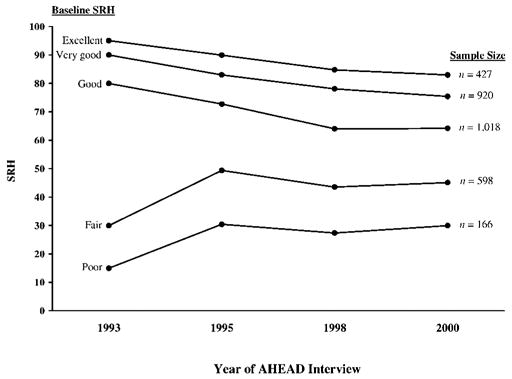
Trends in self-rated health (SRH) and analytic sample size grouped by baseline SRH, based on Diehr and colleagues (2001) interval values. Analytic sample includes only non-proxy respondents in each of the four waves who were still alive in Wave 4 (2000). AHEAD = Asset and Health Dynamics Among the Oldest Old.

Of the 3,129 persons in the analytic sample, 435 (13.9%) were known to have died between the fourth and fifth interview waves. Table 2 presents the results of the four logistic regression models that evaluated the direct effect of current SRH and prior SRH trajectories on mortality. Current SRH (2000) was significant (p < .0001) in all four models. The adjusted odds ratios were extremely robust, ranging only from .981 in Model 2 to .984 in Model 4. Furthermore, for each of the models, the 95% confidence intervals fell between 0.977 and 0.988. These results reflected the impact of a 1-point change in current SRH on subsequent mortality. Because SRH had been transformed to a 0–100-point scale, where the difference between good and fair health was 50 points, these results clearly have substantial clinical relevance.

Table 2.

Adjusted Odds Ratios and Model Fit Statistics for Four Logistic Regression Models to Predict Mortality in 2002

Variablea	Model 1	Model 2	Model 3	Model 4
SRHb (95% confidence interval)	0.981*** (0.977, 0.984)	0.981*** (0.977, 0.984)	0.981*** (0.978, 0.985)	0.984*** (0.980, 0.988)
SRH trajectoryc		0.995	0.993	1.002
SRH trajectory SSEd			1.014*	1.008
Covariatee
Age (years)				1.110***
Men				1.429**
High school graduates				0.726**
Have lung disease				2.115***
Ever smoked				1.350*
Model fit statistic
C statistic	.636	.636	.645	.720
Hosmer–Lemeshowf	.0185	.0132	.0990	.0749

Notes: SRH = self-rated health; SSE = sum of squared errors.

^aBased on baseline (1993) responses, except for SRH (2000), SRH trajectory (1993–1998), and SRH trajectory SSE.

^bBased on Diehr and colleagues (2001) transformation: excellent =95, very good = 90, good = 80, fair = 30, and poor = 15.

^cEqual to −1 times the estimate of the slope parameter from the univariate linear regression of the SRH values over time; a larger number represents a more negative slope or worsening SRH trend.

^dSSE from trajectory regression/100; represents a measure of fit of the calculated trajectory.

^eConfounders shown in table include only those with significant p values. In Model 4, the following nonsignificant variables are also included: race; living alone; income; religiosity; ever drunk alcohol; (ever) had hypertension, diabetes, cancer, hip fracture, heart condition, or stroke; obesity; number of activity of daily living (ADL) and instrumental ADL (IADL) limitations; and prior year hospital admissions, nursing home admissions, and doctor visits. The p values for number of ADL limitations and having a heart condition were each .08; for all other parameter estimates, p > .20.

^fNumber shown is p value of the Hosmer–Lemeshow goodness-of-fit test. p > .05 indicates that one cannot reject the hypothesis of an adequate model fit.

^*p < .05;

^**p < .01;

^***p < .001.

When we introduced the prior SRH trajectory slope measure in Model 2, it was not significant. Moreover, it failed to have a significant association with mortality after adjustment for all of the covariates. The SRH trajectory slope fit measure (SRH trajectory SSE) was significantly associated with mortality when introduced in Model 3 (p < .05), although its effect size was negligible. Furthermore, after adjustment for the covariates in Model 4, the trajectory slope fit measure was no longer significantly associated with mortality. Among the covariates in Model 4, only five were significantly associated with mortality. These were age and sex (risk factors), having had lung disease (health status), having ever smoked (behavior), and being a high school graduate (resource). Of these, only being a high school graduate had a protective effect. Based on the standardized parameter estimates (not shown in Table 2), the two variables in Model 4 having the largest associations with mortality were age and current SRH. The C statistic, a proportional reduction in errors measure (Hanley & McNeil, 1982), increased from .636 in Model 1 to .720 in Model 4. The Hosmer–Lemeshow test statistic (Hosmer & Lemeshow, 2000) p value was not significant in Models 3 and 4, indicating no evidence of heteroscedastic error.

Although the results shown in Table 2 make it clear that prior SRH trajectory has no direct effect on subsequent mortality, it might have an indirect effect through its influence on current SRH. In order to examine this possibility, we regressed current SRH (2000) on the two measures of prior SRH trajectory and the covariates. Table 3 shows these results. Both prior SRH trajectory measures (slope and slope fit) were significant (p < .0001) predictors of current SRH (2000), as were 16 of the covariates. Having higher income, being a high school graduate, living alone, and expecting to live more than 10 years each had a positive effect on current SRH. In contrast, the health status and risk factors, along with doctor visits, all had negative effects.

Table 3.

Parameter Estimates and Model Fit Statistics for Three Regression Models to Predict SRH Status in 2000

Variablea	Model 1	Model 2	Model 3
SRH trajectoryb	−0.862***	−0.626***	−0.846***
SRH trajectory SSEc		−1.127***	−0.713***
Confounderd
High school graduates			3.292**
Live alone			2.613*
Non-White			−3.695*
Religion not very important			−2.614**
Expectation (probability) of living 10 more yearse
0%			−7.020***
51%–99%			3.635**
100%			5.348**
High incomef			3.271**
Ever smoked			−4.051***
CES-D scoreg			−2.129***
Diabetes			−7.268***
Hypertension			−2.809**
Number of ADL limitationsh			−4.944***
Number of IADL limitationsi			−2.905**
Lung disease			−11.523***
Heart condition			−7.943***
Stroke (ever had)			−4.580*
Doctor visitsj			−0.373***
R2	.0344	.0959	.2677

Notes: SRH = self-rated health; SSE = sum of squared errors; CES-D = Center for Epidemiologic Studies–Depression scale; ADL = activity of daily living; IADL = instrumental ADL.

^aBased on baseline (1993) responses, except for SRH trajectory, SRH change 1998–2000, and SRH trajectory SSE.

^bEqual to −1 times the estimate of the slope parameter from the univariate linear regression of the self-rated health values over time; a larger number represents a more negative slope or worsening SRH trend.

^cSSE from trajectory regression/100; represents a measure of fit of the calculated trajectory.

^dConfounders shown in table include only those with significant p values. In Model 3, the following nonsignificant variables are also included: religiosity; ever drunk alcohol; (ever) had cancer or hip fracture; obesity; and prior year hospital admissions and nursing home admissions. The p values for number of ADL limitations and having a heart condition were .07 and .10, respectively; for all other parameter estimates, p > .25.

^eReference category = expected chance of living 10 years is 50%. The parameter estimate for the categorical variable indicating expectations of 1%–49% was not significant.

^fIncome in top fourth or fifth quintile of all 7,447 respondents of the Asset and Health Dynamics Among the Oldest Old survey.

^gSum of “yes” responses for 8 items from the CES-D. A higher score represents more depressive symptoms. Proxy respondents (none in analytic sample) did not answer this question.

^hNumber of ADLs with which respondent needed help or had difficulty (range is 0 to 6).

ⁱNumber of IADLs with which respondent needed help or had difficulty (range is 0 to 5).

^jNumber of times respondent talked to a medical doctor about own health in past 12 months (prior to baseline interview).

^*p < .05;

^**p < .01;

^***p < .001.

DISCUSSION

This article makes two important contributions to the trajectory hypothesis, which Idler and Benyamini (1997) proposed as one of four plausible explanations for the consistently observed relationship between SRH and mortality among older adults. First, we clarified that the trajectory hypothesis actually has two components—one reflecting how one’s health has changed in the past (i.e., a backward-looking trajectory) and the other reflecting how one anticipates that her or his health will change in the future (i.e., a forward-looking trajectory). Second, we specifically evaluated whether prior SRH (i.e., backward-looking) trajectories had independent and direct associations with mortality, or whether those associations were indirect via the influence of prior SRH trajectories on current SRH perceptions. Our analyses of SRH data obtained in 1993, 1995, and 1998 on 3,129 AHEAD respondents clearly showed that prior SRH trajectories did not have a significant, direct effect on mortality between 2000–2002 that was independent of SRH reports obtained in 2000, but that prior SRH trajectories did have an indirect effect on mortality via their substantial influence on current (i.e., 2000) SRH. Further research is needed, however, in order to address the forward-looking component of the trajectory hypothesis.

In concluding this article, it is important to note two limitations of our study: potential selection bias and the use of baseline rather than time-varying respondent characteristics. The most salient of these limitations is selection bias, which has two potential sources. The first results from the fact that individuals in the analytic sample had to have been alive for and participated in four waves of interviews in order for us to predict subsequent mortality. As shown in Table 1, the analytic sample differed from excluded participants in predictable ways. Although the reason for including only those AHEAD participants who survived and were re-interviewed through 2000 is straightforward (i.e., we needed three SRH data points in order to determine the slope and slope fit parameters for each respondent), the result was that all participants in the analytic sample survived for at least 9 years after baseline. This survivor effect was most concentrated among those who reported that their SRH at baseline was fair or poor. Essentially, we effectively constrained those respondents to be false negatives, at least in the short term, with regard to the deleterious effect of poor SRH on mortality.

The second potential source of selection bias involved loss to follow-up between 2000 and 2002. That is, to be included in the analytic sample, AHEAD participants not only had to have survived and been re-interviewed in 1995, 1998, and 2000, but their vital status had to have been determined in 2002. Of the successfully re-interviewed survivors in 2000, 125 were lost to follow-up in 2002. In order to examine the effect of omitting these 125 lost participants, we conducted additional sensitivity analyses. We re-estimated the final model (Model 4 in Table 2), incorporating these 125 respondents under two scenarios. In the first scenario, we assumed these respondents to have been alive in 2002, and in the second scenario, we assumed them to have died. Both scenarios yielded results equivalent to those reported in Table 2.

Our decision to treat the covariates as fixed at baseline is the second limitation of our study. By our using distal (1993) rather than current (2000) values, the effects of the covariates may have been attenuated. This problem would not apply to most variables, as age changes would have been constant for all respondents, sex and race would not have changed, changes in educational attainment would have been minimal, and the only changes in the disease history markers would have reflected incident cases. Changes in living arrangements, income, religiosity, ADLs, IADLs, depressive symptoms, and the use of health services, however, might have resulted in important misclassifications. However, given that our primary focus was on testing the trajectory hypothesis, and given that the trajectory measures were not significantly associated with mortality in Models 2 and 3, it is unlikely that our main conclusions would have been altered.

References

- Benyamini Y, Idler EL. Community studies reporting association between self-rated health and mortality, additional studies, 1995 to 1998. Research on Aging. 1999;21(3):392–401. [Google Scholar]
- Diehr P, Patrick DL, Spertus J, Kiefe CI, McDonell M, Fihn SD. Transforming self-rated health and the SF-36 scales to include death and improve interpretability. Medical Care. 2001;39:670–680. doi: 10.1097/00005650-200107000-00004. [DOI] [PubMed] [Google Scholar]
- Hanley JA, McNeil BJ. The meaning and use of the area under a receiver operating characteristic (ROC) curve. Radiology. 1982;143:29–36. doi: 10.1148/radiology.143.1.7063747. [DOI] [PubMed] [Google Scholar]
- Hosmer DW, Jr, Lemeshow S. Applied logistic regression. 2. New York: Wiley; 2000. [Google Scholar]
- Idler EL, Benyamini Y. Self-rated health and mortality: A review of twenty-seven community studies. Journal of Health & Social Behavior. 1997;38(1):21–37. [PubMed] [Google Scholar]
- Mirowsky J, Ross CE. Education, social status, and health. New York: Aldine de Gruyter; 2003. [Google Scholar]
- Mossey JM, Shapiro E. Self-rated health: A predictor of mortality among the elderly. American Journal of Public Health. 1982;72:800–808. doi: 10.2105/ajph.72.8.800. [DOI] [PMC free article] [PubMed] [Google Scholar]