Team Assembly Mechanisms Determine Collaboration Network Structure and Team Performance

Abstract

Agents in creative enterprises are embedded in networks that inspire, support, and evaluate their work. Here, we investigate how the mechanisms by which creative teams self-assemble determine the structure of these collaboration networks. We propose a model for the self-assembly of creative teams that has its basis in three parameters: team size, the fraction of newcomers in new productions, and the tendency of incumbents to repeat previous collaborations. The model suggests that the emergence of a large connected community of practitioners can be described as a phase transition. We find that team assembly mechanisms determine both the structure of the collaboration network and team performance for teams derived from both artistic and scientific fields.

Teams are assembled because of the need to incorporate individuals with different ideas, skills, and resources. Creativity is spurred when proven innovations in one domain are introduced into a new domain, solving old problems and inspiring fresh thinking (1-4). However, research shows that the right balance of diversity on a team is elusive. Although diversity may potentially spur creativity, it typically promotes conflict and miscommunication (5-7). It also runs counter to the security most individuals experience in working and sharing ideas with past collaborators (8). Successful teams evolve toward a size that is large enough to enable specialization and effective division of labor among teammates but small enough to avoid overwhelming costs of group coordination (9). Here, we investigate empirically and theoretically the mechanisms by which teams of creative agents are assembled. We also investigate how these microscopic team assembly mechanisms determine both the macroscopic structure of a creative field and the success of certain teams in using the resources and knowledge available in the field. We develop a model for the assembly of teams of creative agents in which the selection of the members of a team is controlled by three parameters: (i) the number, m, of team members; (ii) the probability, p, of selecting incumbents, that is, agents already belonging to the network; and (iii) the propensity, q, of incumbents to select past collaborators. The model predicts the existence of two phases that are determined by the values of m, p, and q. In one phase, there is a large cluster connecting a substantial fraction of the agents, whereas in the other phase the agents form a large number of isolated clusters.

We analyzed data from both artistic and scientific fields where collaboration needs have experienced pressures such as differentiation and specialization, internationalization, and commercialization (4, 10, 11): (i) the Broadway musical industry (BMI) and (ii) the scientific disciplines of social psychology, economics, ecology, and astronomy (Table 1). For the BMI, we considered all 2258 productions in the period from 1877 to 1990 (12, 13). Productions are defined as musical shows that were performed at least once in Broadway. The team members comprise individuals responsible for composing the music, writing the libretto and the lyrics, designing the choreography, directing, and producing the show, but not the actors that performed in it. For each of the scientific disciplines, we considered all collaborations that resulted in publications in recognized journals within the fields studied (14): seven social psychology journals, nine economics journals, 10 ecology journals, and six astronomy journals (Table 2). Collaboration networks (15-19) were then built for each of the journals independently and for the whole discipline by merging the data from the journals within a discipline (Materials and Methods).

Table 1.

Global network properties of the fields studied. The sources for the BMI are (12) and (13). The data analyzed excludes revivals and focus on the steady-state period from 1940 to 1985. The data for scientific publications was obtained from the Web of Science. We selected recognized journals in each of the different scientific fields (Table 2). For each field, we show the total number of productions and agents in all the periods considered, the values of p and q estimated with the model from the data, the f_R, the size, N, of the network in the last year of the period considered, the value, N_mod, predicted by the model, the fraction, S, of agents that belong to the largest cluster, and the value, S_mod, predicted by the model. S takes values between 0 and 1 and does not depend on the size of the network (31).

Field	Period	Productions	Agents	p	q	fR	N	Nmod	S	Smod
BMI	1877–1990	2258	4113	0.52	0.77	0.16	428	420	0.70	0.80
Social psychology	1955–2004	16,526	23,029	0.56	0.78	0.22	11,412	14,408	0.68	0.67
Economics	1955–2004	14,870	23,236	0.57	0.73	0.22	9527	11,172	0.54	0.50
Ecology	1955–2004	26,888	38,609	0.59	0.76	0.23	23,166	26,498	0.75	0.84
Astronomy	1955–2004	30,552	30,192	0.76	0.82	0.39	18,021	22,794	0.92	0.98

Table 2.

Journal-specific network structure. We present the same information as in Table 1 for each of the journals studied. We ranked journals within each field according to their impact factor (IF). For some low-impact journals, the f_R is too high to be reproducible with the model. In those cases, which we represent by q > 1, simulations of the model are done with q = 1. The model still reproduces the empirical results quite well for these cases.

Journal	IF	Period	Agents	p	q	fR	S	Smod
Social psychology
J. Pers. Soc. Psychol.	3.862	1965–2003	9112	0.56	0.74	0.20	0.75	0.79
J. Exp. Soc. Psychol.	2.131	1965–2004	2133	0.40	0.76	0.11	0.44	0.07
Pers. Soc. Psychol. B	1.839	1976–2004	4339	0.45	0.74	0.14	0.54	0.47
Eur. J. Soc. Psychol.	1.060	1971–2004	1790	0.41	0.93	0.15	0.44	0.08
J. Appl. Soc. Psychol.	0.523	1971–2004	4602	0.33	1.00	0.10	0.06	0.02
J. Soc. Psychol.	0.291	1956–2004	6294	0.32	>1	0.12	0.05	0.01
Soc. Behav. Personal.	0.227	1973–2004	1981	0.26	>1	0.08	0.03	0.01
Economics
Q. J. Econ.	4.756	1956–2004	2320	0.37	0.58	0.08	0.26	0.05
Econometrica	2.215	1965–2004	3351	0.45	0.67	0.13	0.26	0.05
J. Polit. Econ.	2.196	1956–2004	3464	0.30	0.88	0.07	0.06	0.01
Am. Econ. Rev.	1.938	1956–2004	6807	0.42	0.84	0.15	0.27	0.02
Econ. J.	1.295	1956–2004	4528	0.31	0.99	0.09	0.08	0.01
Eur. Econ. Rev.	1.021	1969–2004	2585	0.35	0.85	0.10	0.15	0.02
J. Econ. Theory	0.833	1969–2004	2062	0.28	>1	0.08	0.51	0.03
Econ. Lett.	0.337	1978–2004	5129	0.31	0.98	0.10	0.01	0.01
Appl. Econ.	0.200	1969–2004	4488	0.26	>1	0.08	0.01	0.01
Ecology
Am. Nat.	4.059	1955–2004	4990	0.44	0.70	0.13	0.49	0.19
Ecology	3.701	1965–2003	8885	0.48	0.71	0.15	0.56	0.65
Oecologia	3.128	1969–2004	10,545	0.44	0.81	0.15	0.51	0.36
Ecol. Appl.	2.852	1991–2004	3417	0.29	0.99	0.08	0.30	0.06
J. Ecol.	2.833	1955–2004	3639	0.43	0.91	0.15	0.40	0.19
Funct. Ecol.	2.351	1989–2004	2873	0.36	>1	0.13	0.05	0.02
Oikos	2.142	1961–2004	6589	0.43	0.84	0.15	0.48	0.11
Biol. Conserv.	2.056	1977–2004	5821	0.27	>1	0.09	0.08	0.01
Ecol. Model.	1.561	1978–2004	5260	0.35	>1	0.13	0.14	0.02
J. Nat. Hist.	0.497	1967–2004	2631	0.36	>1	0.04	0.13	0.01
Astronomy
Astron. J.	5.647	1965–2003	10,832	0.78	0.86	0.40	0.96	0.99
Publ. Astron. Soc. Pac.	3.529	1955–2004	6769	0.58	0.78	0.22	0.85	0.89
Icarus	2.611	1983–2004	4357	0.72	0.90	0.38	0.89	0.97
Publ. Astron. Soc. Jpn.	2.312	1965–2004	2432	0.77	0.95	0.44	0.95	0.99
Astrophys. Space Sci.	0.522	1968–2004	10,823	0.55	1.00	0.29	0.60	0.05
IAU Symp.	0.237	1984–2004	10,185	0.60	0.75	0.23	0.80	0.92

The evolution of team sizes in the BMI bears out the expectation that team size and composition depend on the intricacy of the creative task. In the period from 1877 to 1929, when the form of the Broadway musical show was still being worked out through trial and error (12), there was a steady increase in the number of artists per production, from an average of two to an average of seven (Fig. 1A). This increase in size suggests that teams evolved to manage the complexity of the new artistic form. By the late 1920s, the Broadway musical reached the form we know today, as did team composition (4). Since then, the typical set of artists creating a Broadway musical have been choreographer, composer, director, librettist, lyricist, and producer. For the following 55 years, a period that includes the Great Depression, World War II, and the postwar boom, the average size of teams remained around seven (20).

Fig. 1.

Time evolution of the typical number of team members in (A) the BMI and scientific collaborations in the disciplines of (B) social psychology, (C) economics, (D) ecology, and (E) astronomy.

We find similar scenarios for the evolution of team size in scientific collaborations. The four fields experienced an increase in team size with time (Fig. 1, B to E). The increase has been roughly linear in social psychology and economics and faster than linear in ecology and astronomy. For social psychology, team size growth rate was greater for high-impact compared with low-impact journals, suggesting that team size not only depends on the intricacy of the enterprise but also that successful teams might adapt faster to external pressures.

The analysis of team size cannot capture the fact that teams are embedded in a larger network (3). This complex network (21-26), which is the result of past collaborations and the medium in which future collaborations will develop, acts as a storehouse for the pool of knowledge created within the field. The way the members of a team are embedded in the larger network affects the manner in which they access the knowledge in the field. Therefore, teams formed by individuals with large but disparate sets of collaborators are more likely to draw from a more diverse reservoir of knowledge. At the same time and for the same reasons, the way teams are organized into a larger network affects the likelihood of breakthroughs occuring in a given field.

The agents composing a team may be classified according to their experience. Some agents are newcomers, that is, rookies, with little experience and unseasoned skills. Other agents are incumbents. They are established persons with a track record, a reputation, and identifiable talents. The differentiation of agents into newcomers and incumbents results in four possible types of links within a team: (i) newcomer-newcomer, (ii) newcomer-incumbent, (iii) incumbent-incumbent, and (iv) repeat incumbent-incumbent. The distribution of different types of links reflects the team's underlying diversity. For example, if teams have a preponderance of repeat incumbent-incumbent links, it is less likely that they will have innovative ideas because their shared experiences tend to homogenize their pool of knowledge. In contrast, teams with a variety of types of links are likely to have more diverse perspectives to draw from and therefore to contribute more innovative solutions.

Because quantifying the emergence and the effects of team diversity (2, 9, 27-29) is more difficult than measuring team size, we consider next a model for the assembly of teams. In our model, we assemble N teams in temporal sequence. The assembly of each team is controlled by three parameters: m, p, and q. The first parameter, m, is the number of agents in a team. In our investigations of the model, we considered three situations: (i) keep m constant, (ii) draw m from a distribution, or (iii) use a sequence of m values obtained from the data. For the theoretical analysis of the model, we kept m constant, whereas comparison with an empirical data set was done with the use of the sequence of m(t) values in the corresponding data set.

The second parameter, p, is the probability of a team member being an incumbent. Higher values of p indicate fewer opportunities for newcomers to enter a field. The third parameter, q, represents the inclination for incumbents to collaborate with prior collaborators rather than initiate a new collaboration with an incumbent they have not worked with in the past.

We start at time zero with an endless pool of newcomers. Newcomers become incumbents the first time step after being selected for a team. Each time step t, we assemble a new team and add it to the network (Fig. 2). We select sequentially m(t) different agents. Each agent in a team has a probability, p, of being drawn from the pool of incumbents and a probability, 1 – p, of being drawn from the pool of newcomers. If the agent is drawn from the incumbents' pool and there is already another incumbent in the team, then (i) with probability q the new agent is randomly selected from among the set of collaborators of a randomly selected incumbent already in the team; (ii) otherwise, he or she is selected at random among all incumbents in the network.

Fig. 2.

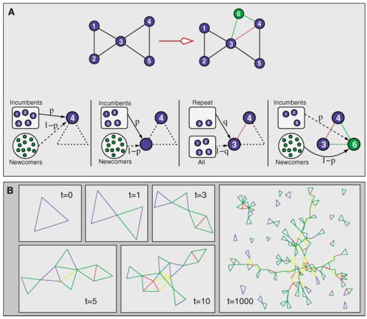
Modeling the emergence of collaboration networks in creative enterprises. (A) Creation of a team with m = 3 agents. Consider, at time zero, a collaboration network comprising five agents, all incumbents (blue circles). Along with the incumbents, there is a large pool of newcomers (green circles) available to participate in new teams. Each agent in a team has a probability p of being drawn from the pool of incumbents and a probability 1 – p of being drawn from the pool of newcomers. For the second and subsequent agents selected from the incumbents' pool: (i) with probability q, the new agent is randomly selected from among the set of collaborators of a randomly selected incumbent already in the team; (ii) otherwise, he or she is selected at random among all incumbents in the network. For concreteness, let us assume that incumbent 4 is selected as the first agent in the new team (leftmost box). Let us also assume that the second agent is an incumbent, too (center-left box). In this example, the second agent is a past collaborator of agent 4, specifically agent 3 (center-right box). Lastly, the third agent is selected from the pool of newcomers; this agent becomes incumbent 6 (rightmost box). In these boxes and in the following panels and figures, blue lines indicate newcomer-newcomer collaborations, green lines indicate newcomer-incumbent collaborations, yellow lines indicate new incumbent-incumbent collaborations, and red lines indicate repeat collaborations. (B) Time evolution of the network of collaborations according to the model for p = 0.5, q = 0.5, and m = 3.

Lastly, agents that remain inactive for longer than τ time steps are removed from the network. This rule is motivated by the observation that agents do not remain in the network forever: agents age and retire, change careers, and so on. The removal process enables the network to reach a steady state after a transient time. Our results do not depend in the specific value of τ (Materials and Methods).

Through participation in a team, agents become part of a large network (30). This fact prompted us to examine the topology of the network of collaborations among the practitioners of a given field. More specifically, we asked, “Is there a large connected cluster comprising most of the agents or is the network composed of numerous smaller clusters?” A large connected cluster would be supporting evidence for the so-called invisible college, the web of social and professional contacts linking scientists across universities proposed by de Solla Price (31) and Merton (32). A large number of small clusters would be indicative of a field made up of isolated schools of thought. For all five fields considered here, we find that the network contains a large connected cluster.

As is typically done in the study of percolation phase transitions (33), we use the fraction S of agents that belong to the largest cluster of the network to quantify the transition between these two regimes: invisible college or isolated schools. We explore systematically the (p,q) parameter space of the model. We find that the system undergoes a percolation transition (33) at a critical line, p_c(m,q). That is, the system experiences a sharp transition from a multitude of small clusters to a situation in which one large cluster, comprising a substantial fraction S of the individuals, emerges: the so-called giant component (Fig. 3). The transition line p_c(m,q) therefore determines the tipping point for the emergence of the invisible college (34). Our analysis shows that the existence of this transition is independent of the average number of agents 〈m〉 in a collaboration, although the precise value of p_c(m,q) does depend on m.

Fig. 3.

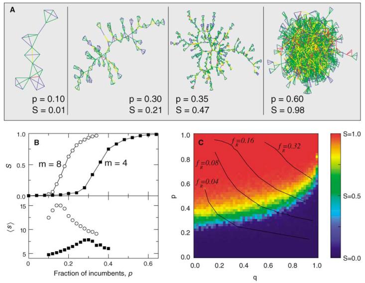
Predictions of the model. (A) Phase transition in the structure of the collaboration network. We plot only the largest cluster in the network. For small p, the network is formed by numerous small clusters (p = 0.10). At the critical point p_c, the tipping point, a large cluster emerges, that is, a cluster that contains a substantial fraction of the agents. In the vicinity of the transition, the largest cluster has an almost linear or branched structure (p = 0.30). As p increases, the largest cluster starts to have loops (p = 0.35) and eventually becomes a densely connected cluster containing essentially all nodes in the network (p = 0.60). We show results for q = 0.5 and m = 4, where m is the number of agents in a team. (B) The transition described in (A) can be characterized by the fraction S of nodes that belong to the giant component, the order parameter, and the average size 〈s〉 of the other clusters, the susceptibility (33). The model displays a second-order percolation transition as the fraction p of incumbents increases from 0 to 1. The transition occurs for p = p_c, which coincides with the maximum of 〈s〉. Note that p_c is a decreasing function of m. We show results for q = 0.5 and m = 4 and m = 8. (C) We display graphically the value of S as a function of p and q for m = 4. For any value of q, the model displays the percolation transition, and the critical fraction p_c depends on q, defining a percolation line p_c(m,q). The critical line p_c(m,q) is an increasing function of q. Even though the order parameter S is an important parameter to quantify the structure of the network, not all points with the same S, that is, all points represented with the same color, correspond to fields with identical properties. This result is made clear by the lines of equal f_R. The upper-right corner of the (p,q) plane is characterized by f_R close to one, whereas the lower-left corner corresponds to f_R close to zero. As we show in Fig. 4, all fields considered have parameter values above the transition line.

The proximity to the transition line, which depends on the distribution of the different types of links, determines the structure of the largest cluster (Fig. 3A). In the vicinity of the transition, the largest cluster has an almost linear or branched structure (Fig. 3A) (p = 0.30). As one moves toward larger p, the largest cluster starts to have more and more loops (Fig. 3A) (p = 0.35), and, eventually, it becomes a densely connected network (Fig. 3A) (p = 0.60).

Networks with the same fraction, S, of nodes in the largest cluster do not necessarily correspond to networks with identical properties. Each point in the (p,q) parameter space is characterized by both S and the fraction, f_R, of repeat incumbent-incumbent links. For example, in Fig. 3C, the line f_R = 0.32 corresponds to those values of p and q for which 32% of all links in new teams are between repeat collaborators (35). The f_R has a notable impact on the dynamics of the network. When f_R is large, collaborations are firmly established, and therefore the structure of the network changes very slowly. In contrast, low values of f_R correspond to enterprises with high turnover and very fast dynamics. Intermediate values of f_R are related to situations in which collaboration patterns with peers are fluid (Materials and Methods).

For each of the five fields for which we have empirical data, we measure the relative size of the giant component S (Materials and Methods). For all fields considered, S is larger than 50% (Table 1). This result provides quantitative evidence for the existence of an invisible college in all the fields. Intriguingly, the relative sizes of the giant component is similar for three of the four fields considered: S = 0.70, S = 0.68, and S = 0.75 for BMI, social psychology, and ecology, respectively. However, for astronomy S was significantly larger (0.92), whereas for economics it was significantly smaller (0.54).

To gain further insight in the structure of collaboration networks, we used our model to estimate the values of p and q for each field. Given the temporal sequence of teams producing the network of collaborations, one can calculate the fraction of incumbents and the fraction of repeat incumbent-incumbent links. These fractions and the model enable us to then estimate the values of p and q that are consistent with the data (36).

We estimated p and q for each field and then simulated the model to predict the key properties of the network of collaborations, including the degree distribution of the network and the fraction S of nodes in the largest cluster. By comparing predictions of the model with the empirical results, we are able to test and validate the model. We first compare the degree distribution of the collaboration networks with the predictions of the model (Fig. 4, A to E) and find that the model predicts the empirical degree distributions remarkably well. In Table 1, we compare the predictions of the model for S with the measured values. The model correctly predicts that an invisible college containing more than 50% of the nodes exists in all cases. Additionally, the values of S predicted by the model are in close agreement with the empirical results.

Fig. 4.

Network structure of different creative fields. Degree distributions for (A) the BMI, (B) the field of social psychology, (C) the field of economics, (D) the field of ecology, and (E) the field of astronomy. We carried out with the use of the sequence {m(t)} of team sizes found in the empirical data and with the values of p and q estimated from the measured fractions of the different types of links. We present the predictions of the model with the lines and the empirical degree distributions with the open circles. For all cases considered, the data falls within the 95% confidence intervals of the predictions of the model. The (p,q) parameter space of the network of collaborators is shown for (F) the BMI, (G) the field of social psychology, (H) the field of economics, (I) the field of ecology, and (J) the field of astronomy. The solid lines separating the red and the blue regions indicate the values of p and q for which 50% of the nodes belong to the largest cluster, that is, the percolation transition at which a giant component, the invisible college, emerges. The distance from the percolation line predicts the overall structure of the network. For example, the networks in astronomy are well above the tipping line and have a very dense structure (Table 1). In contrast, all other fields are close to the transition and have relatively sparse giant components. Another important characteristic of the network is provided by the value of f_R. To help with the interpretation of the results, we plot with dotted lines the curves for f_R = 0.32. For four of the creative networks considered, we find f_R < 0.25. For astronomy, we find f_R = 0.39.

To investigate how changes of the team assembly mechanism affect the structure of the network, we used the model to generate networks with the same sequence of team sizes as the data but with different values of p and q. We show in Fig. 4, F to J, that four out of the five creative networks we consider are very close to the tipping line at which an invisible college emerges. The exception is astronomy. We also find that, for astronomy, the f_R is significantly larger than for the other fields.

If diversity affects team performance and our model correctly captures how diversity is related to the way teams are assembled, then the parameters p and q must be related to team performance. To investigate this issue, we considered for the four scientific fields how teams publishing in different journals are assembled. We used each journal's impact factor as a proxy for the typical quality of teams' output. We then studied the different journals separately to quantify the relationship between team assembly mechanisms and performance.

In Fig. 5, we show the values of p, q, and S for the journals in each of the fields as a function of the impact factor of the journal. We found that p was positively correlated with impact factor for economics, ecology, and social psychology, whereas q was negatively correlated with impact factor for the same fields. The result for p implies that successful teams have a higher fraction of incumbents, who contribute expertise and know-how to the team, whereas the result for q implies that teams that are less diverse typically have lower levels of performance.

Fig. 5.

Relation between team assembly mechanisms, network structure, and performance. We calculate the values of p, q, and S for several journals in each of the four scientific fields considered. In a few cases, q should be larger than one in order to reproduce the empirical values of f_R; in these cases, q is considered one and the corresponding points are shaded. We plot the values of p, q, and S as a function of the impact factor of the journal and then use the Spearman rank-order correlation coefficient r_s to determine significant correlations. Shaded graphs indicate significantly correlated variables at the 95% confidence level.

The relative size S of the giant component in a journal was also associated with performance for ecology and social psychology. Teams publishing in journals with a high-impact factor typically give rise to a large giant component, whereas teams publishing in low-impact journals typically form small isolated clusters. This suggests that teams publishing in high-impact journals perform a better sampling of the knowledge within a field and thus are able to more efficiently use the resources of the invisible college. Surprisingly, neither p, q, or S were significantly correlated with impact factor in astronomy. This distinguishes astronomy from the other creative enterprises considered.

We have shown that team size evolves with time, probably up to an optimal size as in the case of the BMI. A similar process may be occurring for the parameters quantifying expertise, p, and diversity, q. Four of the five fields considered, all except astronomy, have very similar values of p and q, thus suggesting that a “universal” set of optimal values might exist. The fact that in astronomy there are no correlations between p, q, or S and the impact of journals also indicates that this field is different from the others. Whether these differences are caused by the needs imposed by the creative enterprise itself or to historical or other reasons is a question that we cannot answer conclusively.

References and Notes

- 1.Granovetter MS. Am. J. Sociol. 1973;78:1360. [Google Scholar]
- 2.Reagans R, Zuckerman EW. Organ. Sci. 2001;12:502. [Google Scholar]
- 3.Burt R. Am. J. Sociol. 2004;110:349. [Google Scholar]
- 4.Uzzi B, Spiro J. Am. J. Sociol. in press. [Google Scholar]
- 5.Larson JR, Christensen C, Abbott AS, Franz TM. J. Pers. Soc. Psychol. 1996;71:315. doi: 10.1037//0022-3514.71.2.315. [DOI] [PubMed] [Google Scholar]
- 6.Edmondson A. Adm. Sci. Q. 1999;44:350. [Google Scholar]
- 7.Jehn KA, Northcraft GB, Neale MA. Adm. Sci. Q. 1999;44:741. [Google Scholar]
- 8.Stasser G, Stewart DD, Wittenbaum GM. J. Exp. Soc. Psychol. 1995;31:244. [Google Scholar]
- 9.Katzenback JR, Smith DK. The Wisdom of Teams. Harper Business; New York: 1993. [Google Scholar]
- 10.Ziman JM. Prometheus Bound. Cambridge Univ. Press; Cambridge: 1994. [Google Scholar]
- 11.Brown JR. Science. 2000;290:1701. doi: 10.1126/science.290.5497.1701. [DOI] [PubMed] [Google Scholar]
- 12.Green S, Green K. Broadway Musicals Show by Show. ed. 5 Hal Leonard; Milwaukee, WI: 1996. [Google Scholar]
- 13.Simas R. The Musicals No One Came to See: A Guidebook to Four Decades of Musical-Comedy Casualties on Broadway, Off-Broadway and in Out-Of-Town Try-Out, 1943–1983. Garland; New York: 1988. [Google Scholar]
- 14.We imposed several requirements on the journals we selected for analysis. First, the main subject category of the journal must be the desired one. For example, we consider only those ecology journals whose subject category is either ecology or ecology and bio-diversity and conservation according to the Journal Citation Reports. We disregarded more specialized journals, such as Microbial Biology, whose subject category is more specific. We also required that journals contain a sufficiently large number of papers, typically larger than 1000.
- 15.Newman MEJ. Proc. Natl. Acad. Sci. U.S.A. 2001;98:404. [Google Scholar]
- 16.Barabási A-L, et al. Physica A. 2002;311:590. [Google Scholar]
- 17.Newman MEJ. Proc. Natl. Acad. Sci. U.S.A. 2004;101:5200. [Google Scholar]
- 18.Börner K, Maru JT, Goldstone RL. Proc. Natl. Acad. Sci. U.S.A. 2004;101:5266. doi: 10.1073/pnas.0307625100. [DOI] [PMC free article] [PubMed] [Google Scholar]
- 19.Ramasco JJ, Dorogovtsev SN, Pastor-Satorras R. Phys. Rev. E. 2004;70:036106. doi: 10.1103/PhysRevE.70.036106. [DOI] [PubMed] [Google Scholar]
- 20.This stationary state remains until the mid-1980s, when size drops again precisely at the time when a rash of revivals and revues conceivably simplified production.
- 21.Barabasi A-L, Albert R. Science. 1999;286:509. doi: 10.1126/science.286.5439.509. [DOI] [PubMed] [Google Scholar]
- 22.Watts DJ, Strogatz SH. Nature. 1998;393:440. doi: 10.1038/30918. [DOI] [PubMed] [Google Scholar]
- 23.Amaral LAN, Scala A, Barthélémy M, Stanley HE. Proc. Natl. Acad. Sci. U.S.A. 2000;97:11149. doi: 10.1073/pnas.200327197. [DOI] [PMC free article] [PubMed] [Google Scholar]
- 24.Albert R, Barabási A-L. Rev. Mod. Phys. 2002;74:47. [Google Scholar]
- 25.Newman MEJ. SIAM Rev. 2003;45:167. [Google Scholar]
- 26.Amaral LAN, Ottino J. Eur. Phys. J. B. 2004;38:147. [Google Scholar]
- 27.Etzkowitz H, Kemelgor C, Neuschatz M, Uzzi B, Alonzo J. Science. 1994;266:51. doi: 10.1126/science.7939644. [DOI] [PubMed] [Google Scholar]
- 28.Harrison DA, Price KH, Bell MP. Acad. Manage. J. 1998;41:96. [Google Scholar]
- 29.Barsade SG, Ward AJ, Turner JDF, Sonnenfeld JA. Adm. Sci. Q. 2001;46:174. [Google Scholar]
- 30.The teams and the agents are the nodes in a bipartite network. Technically, agents are connected only to teams and vice versa. However, this bipartite network can be projected onto a network comprising only agents and in which there is an edge (connection) between two nodes (agents) if the agents have been connected to at least one common team.
- 31.de Solla Price DJ. Little Science, Big Science… and Beyond. Columbia Univ. Press; New York: 1963. [Google Scholar]
- 32.Merton RK. The Sociology of Science. Univ. of Chicago Press; Chicago: 1973. [Google Scholar]
- 33.Stauffer D, Aharony A. Introduction to Percolation Theory. ed. 2 Taylor and Francis; London: 1992. [Google Scholar]
- 34.Gladwell M. The Tipping Point: How Little Things Can Make a Big Difference. Little, Brown; Boston: 2000. [Google Scholar]
- 35.Figure 3C shows that large fR occurs when p and q are large and corresponds to a network in which collaborations among incumbents are firmly established and opportunities for newcomers are few. Conversely, small fR, which occurs when p and/or q are small, indicates plentiful opportunities for newcomers to join new projects. In this case, newcomers are the norm and collaborations are rarely repeated. Lastly, intermediate values of fR suggest intermediate values of both p and q, that is, a situation for which there is a balance between seasoned incumbents and newcomers with fresh ideas.
- 36.The value of p is directly given by the fraction of incumbents in new creations. The value of q must be obtained numerically by simulating the model with different tentative values of q until the fraction fR of repeat incumbent-incumbent links predicted by the model coincides with the value measured from the data.
- 37.We thank K. Börner, V. Hatzimanikatis, A. A. Moreira, J. M. Ottino, M. Sales-Pardo, and D. B. Stouffer for numerous suggestions and discussions. R.G. thanks the Fulbright Program and the Spanish Ministry of Education, Culture, and Sports. L.A.N.A. gratefully acknowledges the support of a Searle Leadership Fund Award and of a NIH/National Institute of General Medical Studies K-25 award.