Accounting for rate instability and spatial patterns in the boundary analysis of cancer mortality maps

Abstract

Boundary analysis of cancer maps may highlight areas where causative exposures change through geographic space, the presence of local populations with distinct cancer incidences, or the impact of different cancer control methods. Too often, such analysis ignores the spatial pattern of incidence or mortality rates and overlooks the fact that rates computed from sparsely populated geographic entities can be very unreliable. This paper proposes a new methodology that accounts for the uncertainty and spatial correlation of rate data in the detection of significant edges between adjacent entities or polygons. Poisson kriging is first used to estimate the risk value and the associated standard error within each polygon, accounting for the population size and the risk semivariogram computed from raw rates. The boundary statistic is then defined as half the absolute difference between kriged risks. Its reference distribution, under the null hypothesis of no boundary, is derived through the generation of multiple realizations of the spatial distribution of cancer risk values. This paper presents three types of neutral models generated using methods of increasing complexity: the common random shuffle of estimated risk values, a spatial re-ordering of these risks, or p-field simulation that accounts for the population size within each polygon. The approach is illustrated using age-adjusted pancreatic cancer mortality rates for white females in 295 US counties of the Northeast (1970–1994). Simulation studies demonstrate that Poisson kriging yields more accurate estimates of the cancer risk and how its value changes between polygons (i.e. boundary statistic), relatively to the use of raw rates or local empirical Bayes smoother. When used in conjunction with spatial neutral models generated by p-field simulation, the boundary analysis based on Poisson kriging estimates minimizes the proportion of type I errors (i.e. edges wrongly declared significant) while the frequency of these errors is predicted well by the p-value of the statistical test.

1. Introduction

Cancer mortality maps are important tools in health research, allowing the identification of spatial patterns, clusters and disease ‘hot spots’ that often stimulate research to identify potential factors for locally high cancer mortality or morbidity rates (Jacquez, 1998; Rushton et al., 2000). In particular, borders where these cancer mortality or morbidity rates vary abruptly may indicate areas where causative exposures change through geographic space, the presence of local populations with distinct cancer incidences, or the impact of different cancer control methods (Jacquez and Greiling, 2003; Lu and Carlin, 2005). Because of the need to protect patient privacy, publicly available data are often aggregated to a sufficient extent to prevent the disclosure or reconstruction of patient identity. The detection of local boundaries in studies of human populations is thus conducted on areal data, using methods often referred to as areal or polygonal wombling following the seminal work by Womble (1951). Like other pattern recognition approaches, boundary analysis starts with the computation of a statistic that quantifies a relevant aspect of the spatial pattern. Typically a dissimilarity metric (e.g. Manhattan or Euclidian distance) is computed to assess the difference between rates measured in two adjacent geographical units. The observed value of this statistic is then compared to its distribution generated under a null spatial model, for example under the assumption of uniform risk across these two units. This provides a probabilistic assessment of how unlikely an observed spatial pattern is under the null hypothesis. The major weakness of most wombling or edge detection methods currently available is that both the uncertainty attached to the rates and their spatial correlation are ignored in the computation and testing of the boundary statistic.

Mortality rates computed from sparsely populated geographical entities or for diseases with a low frequency of occurrence can be very unreliable. Boundary analysis of raw rates can thus lead to the spurious detection of significant edges in areas of low population density where extreme rates are observed. Simulation studies have demonstrated the benefit of spatial smoothers to obtain more accurate predictions of the underlying risk of cancer. These methods range from simple deterministic techniques (i.e. head banging method, Mungiole et al., 1999) to sophisticated full Bayesian models (Best et al., 2005). Empirical Bayes smoothers (Clayton and Kaldor, 1987) and Poisson kriging (Goovaerts, 2005) provide model-based approaches with intermediate difficulty in terms of implementation and computer requirements. Despite their greater accuracy, risk estimates are still uncertain and this uncertainty should be properly accounted for in the computation and interpretation of the boundary statistic. Since this statistic involves two rates at a time, a measure of joint uncertainty is required in the common situation where these two rates are spatially dependent. Goovaerts (2006) recently developed a geostatistical approach that combines Poisson kriging and p-field simulation to generate multiple realizations of the spatial distribution of risk values. These simulated maps were then fed into local cluster analysis, allowing one to assess how the uncertainty about the spatial distribution of risk values translates into uncertainty about the location of spatial clusters and outliers. Lu and Carlin (2005) proposed a more complex approach based on Bayesian hierarchical models to account for uncertainty in areal wombling procedures.

In many implementations of the wombling approach (e.g. BoundarySeer commercial software), the detection of significant edges is still based on the subjective choice of a relative threshold, say 25%. Edges with a dissimilarity metric in the top 25% are then declared significant regardless of whether the difference between the two rates is statistically significant. Permutation tests were developed to assess the significance of boundaries, for example through subboundary analysis (Oden et al., 1993; Jacquez and Greiling, 2003). However, these tests are based on the hypothesis that each permutation of the observed values is equally likely. In other words, there is an underlying null hypothesis of spatial independence (SI) of observed rates, which is frequently invalidated by the presence of spatial patterns in mortality maps. The term “Neutral Model” captures the notion of a plausible system state that can be used as a reasonable null hypothesis. Goovaerts and Jacquez (2004) described a typology of neutral models that accounts for the spatial dependence of cancer rates, their regional background and spatially heterogeneous population sizes. These models were created using geostatistical simulation and their use in local cluster analysis led to the detection of different clusters and outliers according to the type of hypothesis included in the neutral model.

This paper presents a new geostatistical methodology to account for the instability and spatial patterns of rate data in the detection of significant edges between adjacent polygons. The approach is illustrated using age-adjusted pancreatic cancer mortality rates for white females in 295 US counties of the Northeast (1970–1994). Simulation studies are conducted to compare the performance of the proposed method to common tests based on the null hypothesis of spatial randomness and applied to raw rates or rates stabilized using local empirical Bayes smoothers. Performance criteria include the proportion of edges that are wrongly identified as significant or non-significant, as well as the ability of the significance level of the test to predict the actual proportion of false positives (type I errors).

2. Geostatistical methodology

2.1 The boundary statistic

For a given number N of entities A_α (e.g. counties, states, electoral ward), denote the observed mortality rates as z(u_α)=d(u_α)/n(u_α), where d(u_α) is the number of recorded mortality cases and n(u_α) is the size of the population at risk. These entities are referenced geographically by their centroids with the vector of spatial coordinates u_α=(x_α,y_α). The objective is to detect any significant change between neighboring entities which are here defined as entities sharing a common border or vertex (1-st order queen adjacencies). In this paper, the boundary statistic between any two adjacent entities A_α and A_β is simply defined as half the absolute difference between their corresponding rates:

$${\mathrm{\Delta }}_{\alpha \beta }=\frac{|z(u_{\alpha })–z(u_{\beta })|}{2}$$ (1)

This measure does not account for the shape or size of the two entities, and is not a gradient since the distance between centroids is ignored. By analogy with the local Moran’s I used in local cluster analysis, the boundary statistic (1) can be viewed as a local decomposition of the following global statistic known as madogram in the geostatistical literature:

$${\gamma }_M(h_1)=\frac{1}{2P_1}\sum _{\alpha ,\beta }\left|z(u_{\alpha })–z(u_{\beta })\right|$$ (2)

where P₁ is the number of pairs of entities that share a common border, and h₁ is the average Euclidian distance between their centroids.

2.2 Spatial smoothers

The boundary statistic (1) becomes very unreliable whenever one of the two rates is computed from sparsely populated geographical entities, in particular for diseases with low frequency of occurrence. To correct for the so-called “small number problem”, the observed rates in Equation (1) can be replaced by risk estimates:

$${\mathrm{\Delta }}_{\alpha \beta }^{*}=\frac{|\widehat{r}(u_{\alpha })–\widehat{r}(u_{\beta })|}{2}$$ (3)

A straightforward approach is the local empirical Bayes smoother that estimates the risk at any location u_α as a weighted sum of the rate observed at that location (kernel rate) and a prior local mean:

$${\widehat{r}}_{LEB}(u_{\alpha })=\lambda (u_{\alpha })z(u_{\alpha })+[1–\lambda (u_{\alpha })]m^{*}(u_{\alpha })$$ (4)

where the local mean m* (u_α ) is, for example, a population-weighted average of K neighboring observed rates, including the kernel rate (e.g. see Waller and Gotway, 2004, p. 87). The Bayes shrinkage factor λ(u_α) is computed as:

$$\lambda (u_{\alpha })=\{\begin{array}{cc}\frac{s^2(u_{\alpha })–m^{*}(u_{\alpha })/\overline{n}(u_{\alpha })}{s^2(u_{\alpha })–m^{*}(u_{\alpha })/\overline{n}(u_{\alpha })+m^{*}(u_{\alpha })/n(u_{\alpha })}\hspace{0.17em}\hspace{0.17em}\hspace{0.17em}\hspace{0.17em}& \text{if\hspace{0.17em}}\hspace{0.17em}\hspace{0.17em}{s}^2(u_{\alpha })\ge m^{*}(u_{\alpha })/\overline{n}(u_{\alpha })\\ 0\hspace{0.17em}\hspace{0.17em}\hspace{0.17em}& \text{otherwise}\end{array}$$

where m*(u_α) and s²(u_α) are the population-weighted mean and variance of K neighboring observed rates, and $\overline{n}$(u_α) is the average population size for these K entities. The relative weight λ(u_α) assigned to the kernel rate z(u_α) is smaller for less densely populated entities. For entities with similar population sizes, the factor λ(u_α) is also smaller in areas of greater homogeneity, i.e. characterized by a lower local variance s²(u_α). In other words, where there is less local variability, the estimate (4) tends to be closer to the local mean.

Simulation studies have demonstrated the greater accuracy of risk estimated by Poisson kriging relatively to Bayes smoothers (Goovaerts, 2005). Similarly to the Bayes estimate (4), the Poisson kriging estimate can be expressed as a linear combination of the kernel rate and the rates observed in (K−1) neighboring entities:

$${\widehat{r}}_{PK}(u_{\alpha })=\sum _{i=1}^K{\lambda }_i(u_{\alpha })z(u_i)$$ (5)

where λ_i (u_α) is the weight assigned to the rate z(u_i) when estimating the risk at u_α.The K weights are computed so as to minimize the mean square error of prediction under the constraint that the estimator is unbiased. They are the solution of the following system of linear equations:

$$\begin{array}{l}\sum _{j=1}^K{\lambda }_j(u_{\alpha })\left[C_R(u_i–u_j)+{\delta }_{ij}\frac{m^{*}}{n(u_i)}\right]+\mu (u_{\alpha })=C_R(u_i–u_{\alpha })\hspace{0.17em}\hspace{0.17em}\hspace{0.17em}\text{i}=1,\mathrm{...},K\\ \sum _{j=1}^K{\lambda }_j(u_{\alpha })=1\end{array}$$ (6)

where δ_ij=1 if u_i=u_j and 0 otherwise, and m* is the population-weighted mean of the N rates. The term μ(u_α) is a Lagrange parameter that results from the minimization of the estimation variance subject to the unbiasedness constraint on the estimator. The addition of an “error variance” term, m*/n(u_i), for a zero distance accounts for variability arising from population size, leading to smaller weights for less reliable data (i.e. measured over smaller populations). The prediction variance associated with the estimate (5) is computed using the traditional formula for the ordinary kriging variance:

$${\sigma }_{PK}^2(u_{\alpha })=C_R(0)–\sum _{i=1}^K{\lambda }_i(u_{\alpha })C_R(u_i–u_{\alpha })–\mu (u_{\alpha })$$ (7)

The computation of kriging weights and kriging variance (Equations (6) and (7)) requires knowledge of the covariance of the unknown risk, C_R(h), or equivalently its semivariogram γ_R(h)=C_R(0)−C_R(h). Following Monestiez et al. (2006) the semivariogram of the risk is estimated as:

$${\widehat{\gamma }}_R(h)=\frac{1}{2\sum _{\alpha =1}^{N(h)}\frac{n(u_{\alpha })n(u_{\alpha }+h)}{n(u_{\alpha })+n(u_{\alpha }+h)}}\sum _{\alpha =1}^{N(h)}\left\{\frac{n(u_{\alpha })n(u_{\alpha }+h)}{n(u_{\alpha })+n(u_{\alpha }+h)}{\left[z(u_{\alpha })-z(u_{\alpha }+h)\right]}^2-m^{*}\right\}$$ (8)

where the different pairs [z(u_α)−z(u_α+h)] are weighted by the corresponding population sizes to homogenize their variance. A permissible model, γ_R(h), is then fitted to the experimental semivariogram, i.e. using weighted least-square regression (Pardo-Iguzquiza, 1999) in this paper.

2.3 Probability field simulation

Despite the incorporation of the population size into the computation of the boundary statistic (3), there is always some uncertainty attached to the risk estimates, hence to their differences. In Poisson kriging, the uncertainty about the risk prevailing within an entity A_α is modeled using the Gaussian distribution:

$$F(u_{\alpha };r|(K))=\text{Prob}\{R(u_{\alpha })\le r|(K)\}=G\left(\frac{r-{\widehat{r}}_{PK}(u_{\alpha })}{{\sigma }_{PK}(u_{\alpha })}\right)$$ (9)

where G(.) is the cumulative distribution function of the standard normal random variable. The notation “|(K)” expresses conditioning to the local information, say, K neighboring observed rates. This distribution has a mean and variance corresponding to the Poisson kriging estimate and variance.

In presence of spatial dependence between the risk at u_α and u_β, knowledge of the function (9) does not suffice to characterize the uncertainty attached to the difference (3). A measure of the uncertainty prevailing jointly at locations u_α and u_β is required. This joint uncertainty can be modeled numerically through the simulation of a set of pairs of correlated risk values {(r^(l) (u_α), r^(l) (u_β)), l = 1,..., L}, leading to a set of L simulated values for the boundary statistic {Δ^(l)_αβ ,l =1,..., L}. The ensemble of L simulated values Δ^(l)_αβ is an empirical model of the uncertainty attached to the value of the boundary statistic between A_α and A_β. The mean of the boundary statistic can be computed as the arithmetical average of the L simulated values:

$${\mathrm{\Delta }}_{\alpha \beta }^s=\frac{1}{L}\sum _{l=1}^L{\mathrm{\Delta }}_{\alpha \beta }^{(l)}$$ (10)

At each location u_α the average of simulated risk values, known as E-type estimate, is approximately equal to the kriged risk (Goovaerts, 2006):

$${\widehat{r}}_E(u_{\alpha })=\frac{1}{L}\sum _{l=1}^L{r}^{(l)}(u_{\alpha })\approx {\widehat{r}}_{PK}(u_{\alpha })$$ (11)

Despite the equivalence of the E-type and Poisson kriging estimates, the statistics Δ^*_αβ and Δ^s_αβ are likely different since the absolute value function is convex (Lu and Carlin, 2005), more precisely:

$$\begin{array}{l}{\mathrm{\Delta }}_{\alpha \beta }^s=\frac{1}{L}\sum _{l=1}^L\frac{\left|r^{(l)}(u_{\alpha })-r^{(l)}(u_{\beta })\right|}{2}\\ \ge \frac{1}{2}\left|\frac{1}{L}\sum _{l=1}^L{r}^{(l)}(u_{\alpha })-\frac{1}{L}\sum _{l=1}^L{r}^{(l)}(u_{\beta })\right|=\frac{1}{2}\left|{\widehat{r}}_E(u_{\alpha })-{\widehat{r}}_E(u_{\beta })\right|={\mathrm{\Delta }}_{\alpha \beta }^E\approx {\mathrm{\Delta }}_{\alpha \beta }^{*}\end{array}$$ (12)

Correlated sets of risk values, {r^(l)(u_α), α=1,…,N}, are generated through the sampling of the set of Gaussian distributions of type (9) by a set of spatially correlated probability values {p^(l)(u_α), α = 1,…,N}, known as probability field or p-field. The simulated risk value at u_α is thus generated as:

$$r^{(l)}(u_{\alpha })=F^{-1}(u_{\alpha };p^{(l)}(u_{\alpha })|(K))={\widehat{r}}_{PK}(u_{\alpha })+{\sigma }_{PK}(u_{\alpha })y^{(l)}(u_{\alpha })$$ (13)

where y^(l)(u_α) is the quantile of the standard normal distribution corresponding to the cumulative probability p^(l)(u_α). The L sets of random deviates or normal scores, {y^(l)(u_α), α = 1,…N}, are generated using non-conditional sequential Gaussian simulation which is described in details in Goovaerts (2006).

2.4 Neutral models

Testing the significance of the difference between risks in adjacent entities A_α and A_β amounts at testing whether the boundary statistic is significantly different from zero or not. This test requires the comparison of the observed statistic Δ^*_αβ (or the distribution of simulated statistic values Δ^(l)_αβ ) to a reference distribution generated under a null hypothesis. The term “Neutral Model” captures the notion of a plausible system state that can be used as a reasonable null hypothesis, e.g. the hypothesis of uniform risk. Let {Δ^(j)_{αβ |H0} , j = 1,..., J} be the set of boundary statistic values generated under the null hypothesis H₀. The p-value is the probability that the test statistic takes on a value that is at least as extreme as the observed value when H₀ is true. It is computed as:

$$p_{\alpha \beta }=\frac{1}{J+1}\left(1+\sum _{j=1}^J{i}_{\alpha \beta }^{(j)}\right)$$ (14)

where i^(j)_αβ =1 if the observed boundary statistic exceeds Δ^(j)_αβ|H0, and zero otherwise. When an empirical distribution for the boundary statistic exists, which takes the form of a set of simulated values {Δ^(l)_αβ ,l =1,..., L}, the p-value is computed as:

$$p_{\alpha \beta }=\frac{1}{LJ+1}\left(1+\sum _{l=1}^L\sum _{j=1}^J{i}_{\alpha \beta }^{(lj)}\right)$$ (15)

where i^(lj)_αβ =1 if the simulated statistic Δ^(l)_αβ exceeds Δ^(j)_αβ|H0 , and zero otherwise. The p-value is compared to the significance level chosen by the user and representing the probability of rejecting the null hypothesis when it is true (Type I error). The edge between A_α and A_β is declared significant if the p-value is no greater than the significance level.

The common way to generate the reference distribution under the null hypothesis H₀ of uniform risk is to shuffle randomly the set of observed or smoothed rates, then the boundary statistic is computed for all pairs of adjacent entities, {Δ^(j)_αβ|H0 , ∀ α, β}. This operation is repeated J times, i.e. J=999 in this paper. The main drawback of this randomization procedure is that it implies a typically unrealistic assumption of spatial independence of rates. Intuitively, ignoring the spatial correlation of rates would lead one to overestimate the value of the boundary statistic expected under the null hypothesis, thereby increasing the risk that significant edges go undetected (i.e. larger proportion of false negatives or type II errors).

To account for the spatial pattern of rates the random shuffle can be replaced by the spatially ordered shuffling procedure proposed by Goovaerts and Jacquez (2004). The idea is to generate a standard normal random field with a given spatial covariance, e.g. the covariance of the risk C_R(h), using non-conditional sequential Gaussian simulation. Each simulated normal score is then substituted by the value of same rank in the distribution of observed or smoothed rates. For example, the maximum simulated normal score indicates the location of the maximum observed or smoothed rate in the re-ordered map.

A limitation of the above ordered shuffle is that it ignores the population size within the different geographical units, hence the locally varying reliability of the boundary detection analysis. To account for both the spatial pattern and population sizes, a stochastic simulation procedure similar to the one described in Section 2.3 can be used to generate the neutral models. In this paper, neutral models under the null hypothesis of uniform risk were generated as:

$$r^{(j)}(u_{\alpha }{|\text{H}}_0)=m^{*}+{\sigma }_{PK}(u_{\alpha })y^{(j)}(u_{\alpha })\hspace{0.17em}\hspace{0.17em}\hspace{0.17em}\alpha =1,\dots ,N$$ (16)

where m* is the population-weighted mean of all N rates, and σ_PK(u_α) is the Poisson kriging standard deviation. The J sets of random deviates or normal scores, $\{y^{(j)}(u_{\alpha }),\underset{\dot{}}{\alpha }=1,\dots N\}$, are generated using non-conditional sequential Gaussian simulation.

In summary, three types of neutral models can be generated using the following mechanisms of increasing complexity:

1. Random shuffle of rates, risk estimates or simulated risk values (Model I)

2. Spatially ordered shuffle of rates, risk estimates or simulated risk values (Model II)

3. Probability-field simulation (Model III)

These three types of neutral models correspond to the following three null hypotheses:

1. H₀: uniform and spatially random risk, uniform population size (Model I)

2. H₀: uniform and spatially correlated risk, uniform population size (Model II)

3. H₀: uniform and spatially correlated risk, heterogeneous population size (Model III)

3. Case Study

The new boundary detection method will be illustrated using directly age-adjusted mortality rates for pancreatic cancer. These data are part of the Atlas of Cancer Mortality in the United States (Pickle et al., 1999) and were downloaded from http://www3.cancer.gov/atlasplus/download.html. The rates were adjusted using the 1970 population pyramid. The analysis focuses on rates recorded for white females over the 1970–1994 period for 295 counties of 12 New England States. The population at risk was computed as: 100,000 × the total number of deaths over the 1970–1994 period divided by the age-adjusted cancer mortality rate; both datasets are available on NCI website. Figure 1 (top maps) shows the spatial distribution of age-adjusted mortality rates per 100,000 person-years and the county population at risk.

Figure 1.

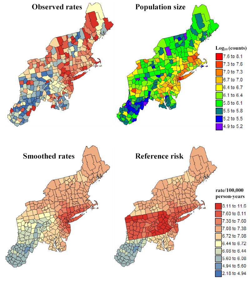
Generation of the reference risk map. The original map of pancreatic cancer mortality rates is first smoothed using a population-weighted kernel, then the rate in each Pennsylvania county is raised by a mortality of 1.45/100,000 person-years. The fill color in each county represents the mortality rate or risk per 100,000 person-years for the period 1970–1994; the class boundaries correspond to the deciles of the histogram of raw rates and the same color scheme is used for all cancer maps.

An objective assessment of performances of the different boundary analyses requires the availability of the underlying risk map and set of “true” boundaries, which are unknown in practice. Simulation provides a way to generate multiple realizations of the spatial distribution of cancer mortality rates under specific scenarios for the underlying risk. The following sections describe the creation of the reference risk map and identification of the set of significant edges, followed by the generation of maps of simulated cancer mortality rates.

3.1 The reference risk map

The reference risk map, {r(u_α), α=1,…,N}, was created in two steps:

1. The original cancer mortality map is smoothed by replacing each rate by the population-weighted average of rates recorded in the 32 closest counties, see Figure 1 (left bottom map). The closeness is measured by the Euclidian distance between the geographic centroids of these counties.

2. The smoothed rate in each county of Pennsylvania is raised by a mortality of 1.45/100,000 person-years, which corresponds to 20% of the population-weighted average of all rates recorded in 295 counties, see Figure 1 (right bottom map).

This operation creates an artificial set of 58 edges that coincide with the Pennsylvania state limits and are referred to as target edges in the subsequent analysis, see Figure 2. Nine additional edges were identified on the original map of smoothed rates based on the value of the boundary statistic (value > 0.3195 deaths per 100,000 person-years) and its spatial gradient (value > 0.7904/100km), see scattergram in Figure 2. The final set of target boundaries thus consists of 67 edges, which represents 8.6% of the total number of pairs of adjacent counties in the dataset.

Figure 2.

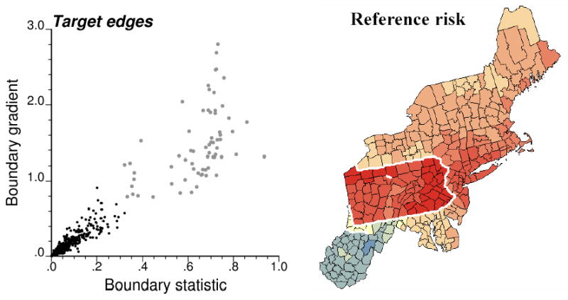
Scattergram of the boundary statistic versus a measure of spatial gradient (i.e. boundary statistic divided by Euclidian distance between centroids) for all 781 pairs of adjacent counties in the New England dataset. Large grey dots depict the target edges that are represented with thick white lines in the reference risk map.

3.2 Simulated maps of mortality rates

Twenty-five maps of simulated rate values were generated from the same underlying risk map of Figure 1 using the Poisson simulation procedure described in Goovaerts (2005). Each map will be considered as a real dataset and undergo the boundary analysis. Although the choice of 25 as number of simulations is somewhat arbitrary, this sample size allows one to reduce statistical fluctuations while processing all scenarios within a reasonable amount of CPU time. The number of cases recorded over each county A_α is simulated by random drawing of a Poisson distribution whose mean parameter is r(u_α)×n(u_α), that is the product of the reference risk by the population size. The simulated rate is computed by dividing the simulated count by the population size. Figure 3 shows the first three realizations generated by this procedure. These rates will be referred to as “raw rates” in the subsequent analysis.

Figure 3.

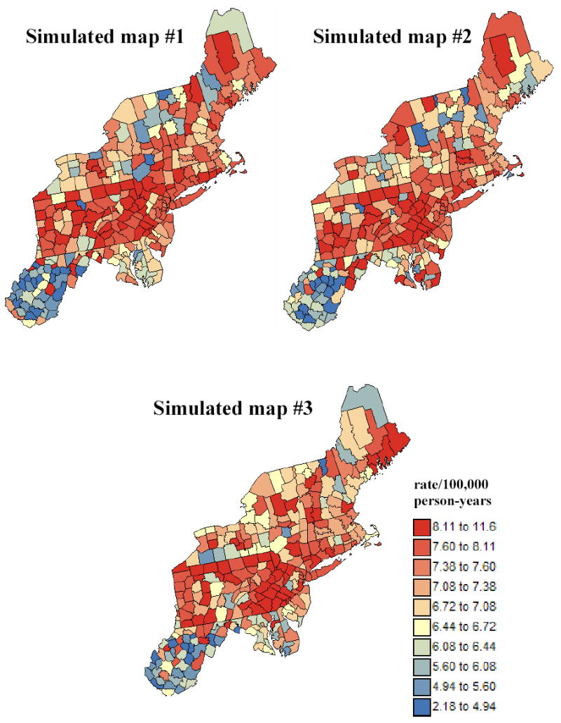
Three realizations of the spatial distribution of pancreatic cancer mortality rates generated using Poisson simulation with the reference risk and population maps displayed in Figure 1. The units are age-adjusted mortality rates per 100,000 person-years.

4. Results and discussion

Each simulated rate map underwent a boundary analysis. Results were compared to the reference risk map and set of target edges shown in Figures 1 and 2. The following four approaches of increasing complexity were implemented:

1. analysis of raw rates

2. analysis of rates smoothed using local empirical Bayes smoother

3. analysis of risk values estimated using Poisson kriging

4. modeling and propagation of uncertainty using p-field simulation (L=100)

Bayes smoothing, Poisson kriging and p-field simulation were performed using the public-domain executables presented in Goovaerts (2005, 2006). Results of the analysis of the first map of simulated rates (Figure 3, left top graph) are displayed in Figures 4 through 7. The experimental risk semivariogram for pancreatic cancer mortality was estimated using equation (8) along four directions. Figure 4 (bottom graph) shows the risk semivariogram, while the traditional semivariogram computed directly from the raw rates is displayed at the top of the Figure. On each graph, the solid curve denotes the model fitted using weighted least-square regression. The weight is the ratio of the square root of the number of data pairs N(h) by the semivariogram value, thereby assigning more importance to the modelling of the semivariogram at the origin. The semivariogram of the risk is much better structured and has a much smaller sill than the corresponding semivariogram of raw rates. This is expected since the weights in expression (8) attenuate the influence of extreme rates computed from small population sizes and subtraction of the correction term m* reduces the variance even more. Accounting for population size in the semivariogram computation reveals a strong anisotropy, with smaller variability along the EW direction of azimuth 90°. Such anisotropy is consistent with the North-South trend exhibited by the reference risk map.

Figure 4.

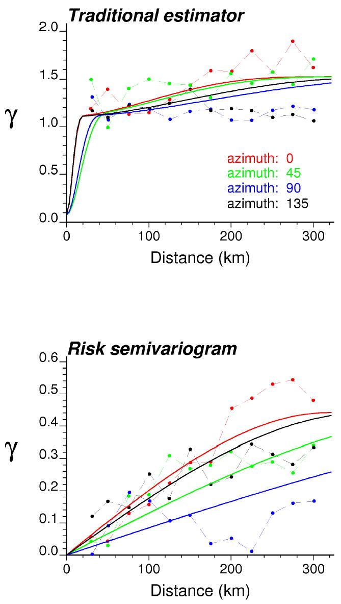
Directional semivariograms for pancreatic cancer mortality rates (realization #1 in Figure 3) computed using the traditional equally-weighted estimator and the risk estimator (Equation 8) that accounts for population size. Azimuth angles are measured in degrees clockwise from the NS axis. The solid curve denotes the anisotropic (i.e. direction-dependent) model fitted using weighted least-square regression.

Figure 7.

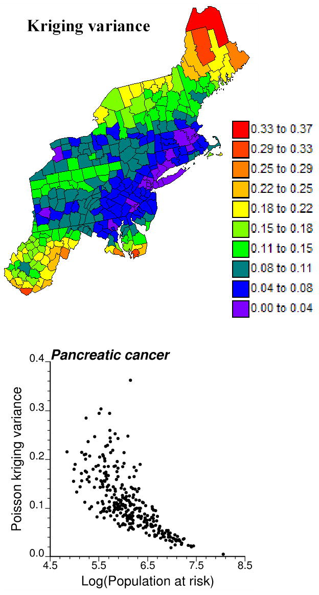
Map of the Poisson kriging variance and scattergram that illustrates the greater uncertainty of the risk estimated for sparsely populated counties.

Figure 5 shows the maps of reference risk values and estimates obtained from the first simulated rate map by application of local empirical Bayes (LEB) smoother, Poisson kriging, and averaging of 100 realizations generated using p-field simulation (E-type estimate). Comparison of the two top maps indicates that the Bayes smoother overestimates the reference risk in the West Virginia and Maryland counties close to the Southwest border of Pennsylvania. Visually, Poisson kriging produces a risk map that is closer to the reference map, which is confirmed by the higher correlation coefficient with reference values (ρ=0.91) than the one computed between reference and LEB risk estimates (ρ=0.86). As expected in theory (Equation 11), the maps of E-type and Poisson kriging estimates are similar (ρ=0.99). Indeed, the p-field realizations are generated by random sampling of Gaussian probability distributions centred on the Poisson kriging estimates, recall Section 2.3.

Figure 5.

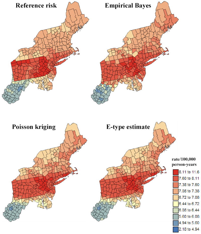
Maps of reference risk values and estimates obtained from the first simulated rate map by application of local empirical Bayes smoother, Poisson kriging, and averaging of 100 realizations generated using p-field simulation (E-type estimate). The units are age-adjusted mortality rates per 100,000 person-years.

Figure 6 shows the first two probability fields (top maps) and the corresponding simulated risk maps. Note the clear EW bands of high and low probabilities, which reflects the anisotropy displayed by the risk semivariogram model in Figure 4. Higher probabilities cause the sampling of the upper tail of local probability distributions, hence the generation of higher risk values in those counties. The map of Poisson kriging variances that define the spread of local probability distributions of risk values is displayed in Figure 7. The scattergram illustrates the higher reliability (i.e. smaller variance) of risk estimates for counties with larger population size.

Figure 6.

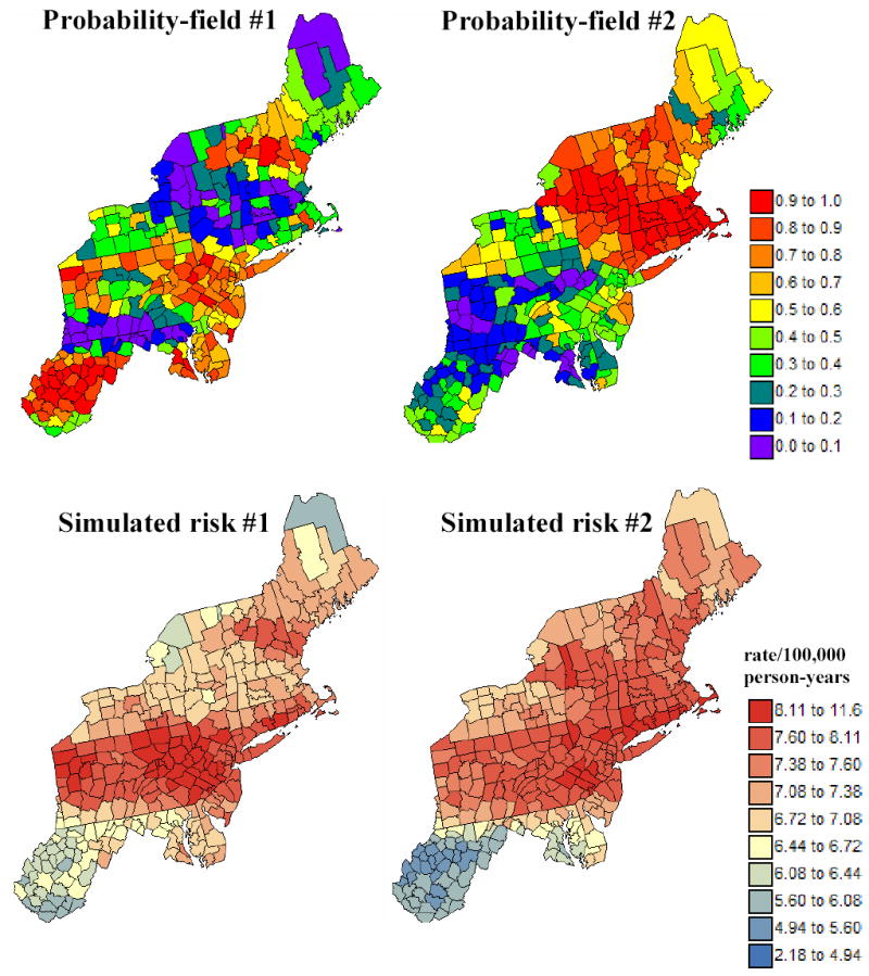
Two simulated maps of probabilities (i.e. probability field) that are used to sample local probability distributions for the risk, generating the two bottom maps of simulated risk values.

4.1 Prediction of the underlying risk

For each of the 25 simulated rate maps, the prediction performance of each approach was quantified using the mean absolute error (MAE) of prediction of risk values defined as:

$$MAE=\frac{1}{295}\sum _{\alpha =1}^{295}|r(u_{\alpha })-r^{*}(u_{\alpha })|$$ (17)

where r(u_α) is the reference risk value for A_α and r*(u_α) is either the raw rate, the local empirical Bayes estimate (Equation 4), the Poisson kriging estimate (Equation 5), or the E-type estimate (Equation 11). Table 1 shows, for each approach, the average and extreme MAE values calculated over the 25 simulated rate maps. Worst results are obtained for the analysis of raw rates. As expected in theory, the E-type and Poisson kriging estimates perform equally. On average, the geostatistical predictors slightly outperform the local empirical Bayes smoother. The benefit of Poisson kriging over the Bayes smoother is however systematic since it leads to smaller prediction errors 92% of the time. All estimators are globally unbiased: the mean of estimated risk values is close to the mean of the reference risk map, see Table 2. The largest bias, albeit small, is caused by the local empirical Bayes smoother that tends to overestimate the risk values, which confirms the visual interpretation of the maps of Figure 5.

Table 1.

Mean absolute error (MAE) of prediction for four alternate predictors. The average, minimum and maximum value calculated over 25 simulated rate maps are reported. The last column gives the percentage of simulations where the MAE for the geostatistical methods is lower than for the local empirical Bayes smoother.

Predictor	Average	Minimum	Maximum	% best prediction
Raw rates	0.6984	0.6413	0.7467
Empirical Bayes	0.2584	0.2252	0.2916
Poisson kriging	0.2345	0.1961	0.2740	92
E-type estimate	0.2348	0.1967	0.2750	92

Table 2.

Average of the reference risk values and the estimates obtained using four alternate approaches. The average, minimum and maximum value of the statistic calculated over 25 simulated rate maps are reported.

Predictor	Average	Minimum	Maximum
Reference risk	7.209	-	-
Raw rates	7.210	7.083	7.295
Empirical Bayes	7.303	7.227	7.364
Poisson kriging	7.242	7.165	7.300
E-type estimate	7.242	7.164	7.300

4.2 Prediction of the boundary statistic

To investigate how the prediction accuracy of the risk value influences the prediction of the boundary statistic (1), the mean absolute error of prediction of that statistic was computed as:

$$MAE=\frac{1}{P_1}\sum _{\alpha ,\beta }\left|{\mathrm{\Delta }}_{\alpha \beta }-{\mathrm{\Delta }}_{\alpha \beta }^{\text{est}}\right|\mathrm{\hspace{0.17em} }\mathrm{\hspace{0.17em} }\mathrm{\hspace{0.17em} }\text{with\hspace{0.17em}}\hspace{0.17em}\hspace{0.17em}{\mathrm{\Delta }}_{\alpha \beta }=\frac{|r(u_{\alpha })-r(u_{\beta })|}{2}$$ (18)

where Δ^est_αβ is the boundary statistic computed from either the raw rates, the local empirical Bayes estimates (Equation 4), the Poisson kriging estimates (Equation 5), or the E-type estimates ( Δ^*_αβ in Equation 12). The MAE statistic is also computed using the average of simulated boundary values ( Δ^s_αβ in Equation 10). Table 3 shows, for each approach, the average and extreme MAE values calculated over the 25 simulated rate maps. The ranking of methods is similar for criteria (17) and (18): Poisson kriging provides more accurate predictions than local empirical Bayes smoother for all but one simulations (24/25). The last two lines in this Table indicate that estimating the boundary statistic from the average of simulated risk values (i.e. E-type estimates) is more accurate than averaging simulated values of the boundary statistic. This result disagrees with the findings in Lu and Carlin (2005). The culprit for the poorer performance of the simulation approach is the overestimation of the boundary statistic: the average value of Δ^s_αβ over all counties and simulations is 0.1329, which is much larger than the reference value of 0.1019, see Table 4. It is also much larger than the average value of the statistic Δ^*_αβ (0.0938), which is expected according to expression (12). In other words, the simulation approach overestimates the local variability of the risk, which might be caused by the use of a very smooth reference risk map in this simulation study. Poisson kriging results are the closest to the reference value, with a slight underestimation of the boundary statistic. Local empirical Bayes smoother overestimates the value of the boundary statistic, though to a lesser extent than the statistic Δ^s_αβ . The erratic fluctuations caused by the small number problem leads to a boundary statistic, computed from raw rates, that is five times larger than the reference value.

Table 3.

Mean absolute error (MAE) of prediction of the boundary statistic by five alternate estimators. The average, minimum and maximum MAE calculated over 25 simulated rate maps are reported. The last column gives the percentage of realizations where the MAE for the geostatistical methods is lower than for the local empirical Bayes smoother.

Predictor	Average	Minimum	Maximum	% best prediction
Raw rates	0.4556	0.4178	0.4907
Empirical Bayes	0.1027	0.0830	0.1199
Poisson kriging	0.0890	0.0809	0.0985	96
Statistic ΔEαβ	0.0890	0.0807	0.0982	96
Statistic Δsαβ	0.1074	0.0925	0.1287	28

Table 4.

Average of the reference boundary statistic values and the estimates obtained using five alternate approaches. The average, minimum and maximum value of the statistic calculated over 25 simulated rate maps are reported.

Predictor	Average	Minimum	Maximum
Reference value	0.1019
Raw rates	0.5263	0.4826	0.5664
Empirical Bayes	0.1200	0.0954	0.1476
Poisson kriging	0.0937	0.0742	0.1187
Statistic ΔEαβ	0.0938	0.0743	0.1189
Statistic Δsαβ	0.1329	0.0990	0.1750

4.3 Detection of target edges

For the five types of estimators compared in Table 2, the significance of the boundary statistic was tested using neutral models (J=999) generated by the three following mechanisms described in Section 2.4:

1. Random shuffle of rates, risk estimates or simulated risk values (Model I)

2. Spatially ordered shuffle of rates, risk estimates or simulated risk values (Model II)

3. Probability-field simulation (Model III)

In each case, a p-value p_αβ is computed for every pair of adjacent counties A_α and A_β, and the corresponding edge is declared significant if p_αβ does not exceed a given significance level α₀. Two types of errors could then occur: misclassification of a non-target edge as significant (type I error or false positive) and misclassification of a target edge as non-significant (type II error or false negative).

Regardless of the choice of a significance level, it is worth comparing approaches according to the order of detection of the 67 target edges. For the neutral models I to III, these 67 edges were ranked according to increasing p-value, that is starting with the most easily detected edge. The boundary analysis was conducted on the raw rates, the local empirical Bayes and Poisson kriging estimates, and the simulated risk values. Each edge is characterized by the following two quantities: the value of the “true” boundary statistic computed from reference risk values, and the average population size of the two adjacent counties. The results were averaged over the set of 25 simulated rate maps, and they are plotted versus the relative order of detection in Figure 8. Poisson kriging and p-field simulation lead to the early detection of edges between counties with the largest differences in the underlying risk values, i.e. largest value of the “true” boundary statistic. The change in the value of the boundary statistic between the first and second half of target edges is particularly pronounced under neutral model III. The analysis of raw or smoothed rates does not allow one to discriminate between edges with large or small change in risk values (i.e. flat curve). When the boundary analysis is conducted on population-based estimates (i.e. smoothed rates, kriged or simulated risks), the target edges that separate the most densely populated counties are detected first, see Figure 8 (right column). The impact of the population size on the order of detection increases from neutral model I to III, with a strong effect when the uncertainty about the boundary statistic (p-field simulation approach) is accounted for under neutral model III.

Figure 8.

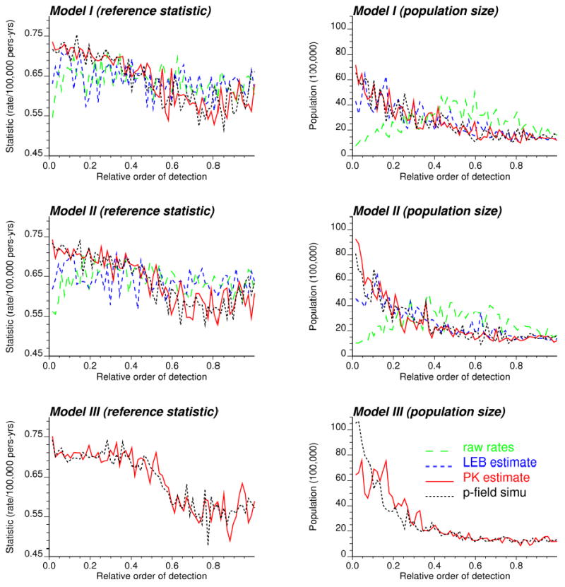
Characteristics (value of the reference boundary statistic and population of adjacent counties) of the target edges detected using four estimators for the boundary statistic: raw rates, smoothed (LEB) rates, risk values estimated by Poisson kriging or simulated by the p-field approach. The edges are ordered according to increasing p-value calculated under neutral models I through III: edges with low p-values are detected first. Results are averaged over the 25 maps of simulated rates.

4.4 Receiver Operating Characteristics Curves

Detection of target edges that have higher p-values requires the use of higher significance levels, thereby increasing the risk of type I error or false positive. The most efficient algorithm is the one that allows the detection of a larger fraction of target edges at the expense of fewer false positives. This information can be summarized in Receiver Operating Characteristics (ROC) curves that plot the probability of false positive versus the probability of detection (Swets, 1988). The probability of detection corresponds here to the proportion of target edges that are detected as the significance level increases. In practice, 67 significance levels, corresponding to the p-values of the 67 target edges, are selected. For each of them the probability of false positive is computed as the proportion of non-target edges that are wrongly declared significant. Figure 9 (left column) shows the ROC curves obtained for the three types of neutral models and various estimators for the boundary statistic. Note that the neutral model III can be applied only to geostatistical estimators. Results are averaged over the 25 maps of simulated rates.

Figure 9.

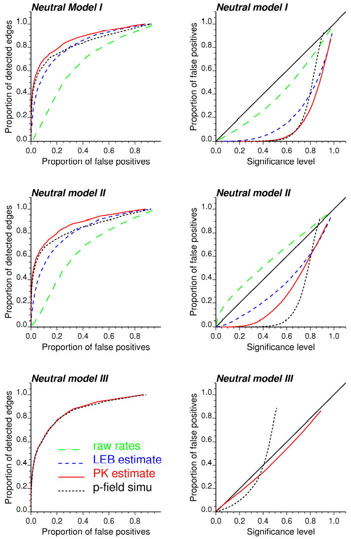
ROC curves (left column) and scattergrams of the expected versus actual proportions of false positives (right column) calculated using three types of neutral models and four estimators for the boundary statistic. Results are averaged over the 25 maps of simulated rates.

A quantitative measure of the detection efficiency is the relative area above the ROC curve, which represents the average proportion of false positives. The smaller this value, the better the detection algorithm. Table 5 shows, for each approach, the average and extreme values of the proportion of false positives calculated over the 25 simulated rate maps. The ranking of approaches is similar for neutral models I and II: raw rates cause the largest proportion of false positives, while the fewest errors are obtained using Poisson kriging. The p-field simulation approach outperforms Bayes smoothers for the early detection of target edges. The two geostatistical approaches are the only ones to benefit slightly from the use of spatial neutral models (type II) over complete randomization (type I). In agreement with the results obtained for the boundary MAE statistic (Table 3), accounting for the uncertainty attached to the boundary statistic through p-field simulation generates more false positives than the more straightforward and less CPU intensive Poisson kriging. Differences between both approaches become negligible when using neutral model III that accounts for population size.

Table 5.

Average proportion of false positives necessary to the detection of all 67 target edges using three types of neutral models and four estimators for the boundary statistic. The average, minimum and maximum proportions calculated over 25 simulated rate maps are reported. The last column gives the percentage of simulations where the particular method yields the smallest proportion of false positives.

Predictor	Average	Minimum	Maximum	% best results
	Neutral Model I
Raw rates	33.0	24.8	43.7	0
Empirical Bayes	17.2	9.63	27.4	4
Poisson kriging	12.7	7.39	18.2	16
Statistic Δsαβ	15.9	10.3	20.4	0
	Neutral Model II
Raw rates	34.0	26.5	45.1	0
Empirical Bayes	18.5	10.7	29.1	0
Poisson kriging	12.3	6.86	18.4	68
Statistic Δsαβ	15.3	10.9	21.4	0
	Neutral Model III
Poisson kriging	13.2	7.00	19.5	8
Statistic Δsαβ	13.2	6.84	20.3	4

4.5 Goodness of the probabilistic model

In addition to minimizing the proportion of false positives, the boundary analysis should provide a reliable estimate of the risk of these type I errors. In other words, the significance level should be as close as possible to the actual proportion of edges that are wrongly declared significant. For each ROC curve displayed in Figure 9, the expected and actual proportions of false positives, denoted F_i and F_i^*, were computed for significance levels corresponding to the p-values of the test for the 67 target edges. The scatterplots of the two sets of proportions are displayed in Figure 9 (right column); the 45 degree line represents the best case scenario. The agreement between both sets of values can be quantified using the goodness statistic (Goovaerts, 2001) defined as:

$$G=1-\frac{1}{67}\sum _{i=1}^{67}{\omega }_i|F_i-F_i^{*}|$$ (19)

where ω_i =1 if F_i^* < F_i, and 2 otherwise. Twice more importance is given to deviations when the proportion of false positives is higher than expected according to the significance level. Table 6 shows, for each approach, the average and extreme values of the goodness statistic calculated over the 25 simulated rate maps. The corresponding average p-value of the tests conducted for target and non-target edges are reported in Table 7.

Table 6.

Goodness statistic measuring the agreement between the actual proportion of false positives and the significance level used in tests based on three types of neutral models and four estimators for the boundary statistic. The average, minimum and maximum values calculated over 25 simulated rate maps are reported. The last column gives the percentage of simulations where the particular method yields the largest goodness statistic.

Predictor	Average	Minimum	Maximum	% best results
	Neutral Model I
Raw rates	0.898	0.873	0.919	0
Empirical Bayes	0.676	0.605	0.713	0
Poisson kriging	0.554	0.450	0.628	0
Statistic Δsαβ	0.561	0.472	0.629	0
	Neutral Model II
Raw rates	0.822	0.718	0.945	0
Empirical Bayes	0.877	0.814	0.927	0
Poisson kriging	0.772	0.691	0.817	0
Statistic Δsαβ	0.605	0.532	0.656	0
	Neutral Model III
Poisson kriging	0.969	0.883	0.994	96
Statistic Δsαβ	0.914	0.857	0.953	4

Table 7.

Average p-value for the tests conducted over the sets of target and non-target edges. The average, minimum and maximum values calculated over 25 simulated rate maps are reported. The last column reports the ratio of average p-values for non-target versus target edges.

Predictor	Target edges			Non-target edges			Contrast
	Aver.	Min.	Max.	Aver.	Min.	Max.
	Neutral Model I
Raw rates	0.432	0.255	0.575	0.599	0.209	0.918	1.38
Empirical Bayes	0.496	0.216	0.883	0.801	0.381	0.966	1.62
Poisson kriging	0.573	0.275	0.872	0.856	0.516	0.961	1.49
Statistic Δsαβ	0.596	0.312	0.858	0.808	0.558	0.921	1.36
	Neutral Model II
Raw rates	0.251	0.106	0.433	0.420	0.084	0.843	1.67
Empirical Bayes	0.308	0.049	0.756	0.657	0.206	0.920	2.13
Poisson kriging	0.351	0.088	0.727	0.723	0.292	0.883	2.06
Statistic Δsαβ	0.544	0.273	0.813	0.772	0.505	0.894	1.42
	Neutral Model III
Poisson kriging	0.141	0.001	0.578	0.532	0.037	0.855	3.76
Statistic Δsαβ	0.159	0.001	0.428	0.399	0.079	0.494	2.51

Under neutral model I, the p-values of the tests based on the two geostatistical approaches are unrealistically large and fail to predict the small proportion of false positives. The best agreement is found for the boundary analysis of raw rates, but it simply means that the p-value correctly predicts the large number of false positives generated by this approach, e.g. average = 0.432 for target edges and 0.599 for non-target edges. The use of spatial neutral models II increases the goodness statistic for all approaches, at the exception of the analysis of raw rates that now understates the actual proportion of false positives. Indeed, accounting for spatial correlation between rates in the generation of neutral models leads to smaller simulated values of the boundary statistic (i.e. reference distribution of the test statistic is shifted to the left), hence a reduction in the magnitude of p-values relatively to neutral model I, see Table 7. The contrast between target and non-target edges also improved under neutral model II. There is very good agreement between expected and actual proportions of false positives when the statistic Δ^*_αβ based on Poisson kriging estimates is used in conjunction with neutral model III. The average goodness statistic is 0.969 and there is a strong contrast between the average p-value of the tests conducted for target and non-target edges: 0.141 versus 0.532. This approach outperforms all others for 24 out of 25 simulations, and it is worth noting it also yields the second smallest proportions of false positives, recall Table 5.

Conclusions

The analysis and interpretation of cancer mortality or incidence maps is frequently hampered by the presence of extreme values caused by the estimation of rates from sparsely populated geographic entities. This problem is particularly stringent whenever rare cancers or minority populations are studied. Smoothers, such as the median-based head banging or empirical Bayes estimators, are routinely applied to stabilize rates. Yet, these methods fail to account for the fact that rates measured in entities that are close in the geographic space tend to be more similar than the ones recorded further apart. Recently, geostatistical variography and prediction were tailored to the situation where the data are composed of a numerator (i.e. death counts) and a denominator (i.e. population size). A form of kriging of data with varying measurement errors, called Poisson kriging, was developed to account for population size in the estimation of risk values from observed rates. The algorithm is easy to implement and the risk semivariogram can be calculated from raw rates using a population-weighted estimator. The simulation study in this paper confirmed that the geostatistical approach systematically outperforms empirical Bayes smoothers for the estimation of cancer risks.

Mapping rates of cancer mortality or incidence is often a preliminary step towards the detection of local areas of excess and deficit, which may guide future surveillance and control activities. Local cluster analysis aims to detect either aggregates of entities with significantly higher or lower cancer risk (i.e. clusters), or single entities that differ significantly from their neighbors (i.e. anomalies). Boundary analysis allows a finer analysis by considering two entities at a time, leading to the detection of significant changes or edges. The significance of both the cluster and boundary statistics is typically assessed under the assumption of independence of rates and without a proper account of the underlying population size. Studies have shown that ignoring spatial dependence in local cluster analysis can lead to over-identification of the number of significant spatial clusters or outliers. Unlike the cluster analysis that relies on a measure of similarity, boundary analysis is based on a dissimilarity metric whose reference value under the null hypothesis of uniform risk is overestimated whenever the spatial autocorrelation of rates is not incorporated in the generation of neutral models. This paper presented p-field simulation as an innovative way to account for both population size and spatial patterns in the generation of more realistic neutral models. The use of these models in statistical tests greatly reduces the magnitude of p-values that reflects better the frequency of false positives. Fewer errors were also committed when the analysis was conducted on the risks estimated by Poisson kriging.

The use of p-field simulation to propagate the uncertainty through the computation of the boundary statistic did not improve over the most straightforward Poisson kriging. The boundary statistic estimates were less accurate and the ROC curves revealed a larger proportion of type I errors for the simulation approach when the neutral models were generated by random or spatially constrained shuffling. Under the most complex neutral model of type III, differences between the kriging and simulation approaches became negligible. Yet, the availability of multiple simulated risk maps makes possible statistical inference regarding the existence of connected strings of significant edges. In other words, the probability for multiple edges to be jointly significant under the null hypothesis of uniform risk could be numerically approximated from the set of spatially correlated risk values.

References

- Best N, Richardson S, Thomson A. A comparison of Bayesian spatial models for disease mapping. Statistical Methods in Medical Research. 2005;14:35–59. doi: 10.1191/0962280205sm388oa. [DOI] [PubMed] [Google Scholar]
- Clayton DG, Kaldor J. Empirical Bayes estimates of age-standardized relative risks for use in disease mapping. Biometrics. 1987;43:671–681. [PubMed] [Google Scholar]
- Goovaerts P. Geostatistical modelling of uncertainty in soil science. Geoderma. 2001;103:3–26. [Google Scholar]
- Goovaerts P. Geostatistical analysis of disease data: estimation of cancer mortality risk from empirical frequencies using Poisson kriging. International Journal of Health Geographics. 2005;4:31. doi: 10.1186/1476-072X-4-31. [DOI] [PMC free article] [PubMed] [Google Scholar]
- Goovaerts P. Geostatistical analysis of disease data: visualization and propagation of spatial uncertainty in cancer mortality risk using Poisson kriging and p-field simulation. International Journal of Health Geographics. 2006;5:7. doi: 10.1186/1476-072X-5-7. [DOI] [PMC free article] [PubMed] [Google Scholar]
- Goovaerts P, Jacquez GM. Accounting for regional background and population size in the detection of spatial clusters and outliers using geostatistical filtering and spatial neutral models: the case of lung cancer in Long Island, New York. International Journal of Health Geographics. 2004;3:14. doi: 10.1186/1476-072X-3-14. [DOI] [PMC free article] [PubMed] [Google Scholar]
- Jacquez, G. (1998). GIS as an enabling technology. In GIS and Health, A. Gatrell and M. Loytonen (eds), Taylor and Francis, London. pp. 17–28.
- Jacquez GM, Greiling DA. Geographic boundaries in breast, lung and colorectal cancers in relation to exposure to air toxics in Long Island, New York. International Journal of Health Geographics. 2003;2:4. doi: 10.1186/1476-072X-2-4. [DOI] [PMC free article] [PubMed] [Google Scholar]
- Lu H, Carlin BP. Bayesian areal wombling for geographical boundary analysis. Geographical Analysis. 2005;37:265–285. [Google Scholar]
- Monestiez P, Dubroca L, Bonnin E, Durbec JP, Guinet C. Geostatistical modelling of spatial distribution of Balenoptera physalus in the Northwestern Mediterranean Sea from sparse count data and heterogeneous observation efforts. Ecological Modelling. 2006;193:615–628. [Google Scholar]
- Mungiole M, Pickle LW, Hansen Simonson K. Application of a weighted head-banging algorithm to mortality data maps. Statistics in Medicine. 1999;18:3201–3209. doi: 10.1002/(sici)1097-0258(19991215)18:23<3201::aid-sim310>3.0.co;2-u. [DOI] [PubMed] [Google Scholar]
- Oden NL, Sokal RR, Fortin MJ, Goebl H. Categorical wombling: detecting regions of significant change in spatially located categorical variables. Geographical Analysis. 1993;25:315–336. [Google Scholar]
- Pardo-Iguzquiza E. VARFIT: a Fortran-77 program for fitting variogram models by weighted least squares. Computers and Geosciences. 1999;25:251–261. [Google Scholar]
- Pickle LW, Mungiole M, Jones GK, White AA. Exploring spatial patterns of mortality: the new Atlas of United States mortality. Statistics in Medicine. 1999;18:3211–3220. doi: 10.1002/(sici)1097-0258(19991215)18:23<3211::aid-sim311>3.0.co;2-q. [DOI] [PubMed] [Google Scholar]
- Rushton G, Elmes G, McMaster R. Considerations for improving geographic information system research in public health. Journal of the Urban and Regional Information Systems Association. 2000;12:31–49. [Google Scholar]
- Swets JA. Measuring the accuracy of diagnostic systems. Science. 1988;240:1285–1293. doi: 10.1126/science.3287615. [DOI] [PubMed] [Google Scholar]
- Waller, L.A. and Gotway, C.A. (2004). Applied Spatial Statistics for Public Health Data, John Wiley and Sons, New Jersey.
- Womble W. Differential systematics. Science. 1951;114:315–322. doi: 10.1126/science.114.2961.315. [DOI] [PubMed] [Google Scholar]