Automated segmentation of the actively-stained mouse brain using multi-spectral MR microscopy

Abstract

Magnetic Resonance Microscopy (MRM) has created new approaches for high-throughput morphological phenotyping of mouse models of diseases. Transgenic and knockout mice serve as a test bed for validating hypotheses that link genotype to the phenotype of diseases, as well as developing and tracking treatments. We describe here a Markov Random Fields based segmentation of the actively-stained mouse brain, as a prerequisite for morphological phenotyping. Active staining achieves higher signal to noise ratio (SNR) thereby enabling higher resolution imaging per unit time than obtained in previous formalin-fixed mouse brain studies. The segmentation algorithm was trained on isotropic 43-micron T1- and T2-weighted MRM images. The mouse brain was segmented into 33 structures, including the hippocampus, amygdala, hypothalamus, thalamus, as well as fiber tracts and ventricles. Probabilistic information used in the segmentation consisted of a) intensity distributions in the T1- and T2-weighted data, b) location, and c) contextual priors for incorporating spatial information. Validation using standard morphometric indices showed excellent consistency between automatically- and manually-segmented data. The algorithm has been tested on the widely used C57BL/6J strain, as well as on a selection of six recombinant inbred BXD strains, chosen especially for their largely-variant hippocampus.

Introduction

Magnetic Resonance Microscopy (MRM) has become a routine imaging modality for a spectrum of mouse models of human neurological conditions. By studying the morpholgy of the brain in transgenic and knockout models of mice (Deng and Siddique 2000); (Price, Wong et al. 2000; Wong, Cai et al. 2002; Hashimoto, Rockenstein et al. 2003), one can obtain insight into the role of genetics and environment in the brain and its response to disease. MRM, with spatial resolution at 10–100 microns, provides a unique non-destructive, three-dimensional (3D) representation of anatomical structures. Numerous studies have demonstrated the value of 3D MR morphometry in mouse models (McDaniel, Sheng et al. 2001; Redwine, Kosofsky et al. 2003; Wilson, Petrik et al. 2004; Cyr, Caron et al. 2005; Bock, Kovacevic et al. 2006).

Most of the previous morphometric studies on the mouse brain have relied on manual and semi-automated methods to identify and delineate structures. Manual segmentations are tedious, error-prone, and are not scalable to larger studies. Automated segmentation in the mouse brain has received attention in the context of 3D probabilistic MR atlases. Several groups have addressed segmentation in the mouse brain as a registration problem (Kovacevic, Henderson et al. 2005); (Iosifescu, Shenton et al. 1997; Ma, Hof et al. 2005; Bock, Kovacevic et al. 2006). The approach has been to manually trace structures on a reference brain volume, non-linearly register the reference brain to the test brain, and then transfer the labels using the warp resulting from the grayscale registration. The standard reference brain consists of a single representative brain that has been selected from a group of brains, which are artifact-free and intact (Ma, Hof et al. 2005), or an averaged result from a group of brains (Kovacevic, Henderson et al. 2005). Segmentation of new brains was accomplished in the latter case, following iterative steps of non-linear registration between a continuously updated reference brain and the target brains. Labels were then transferred from the atlas to new brains. In the work by Ma et al. (Ma, Hof et al. 2005), a T2*-weighted brain scan was used as the reference brain. This single brain was labeled into 20 structures. The reference brain and its labels were then non-linearly registered into the target brains. This provided an initial ‘pilot’ segmentation of the brains, after which the labels were manually corrected for more accurate labeling.

These approaches have potential drawbacks. Registration errors can cause structure mismatches and unevenness of boundaries, for which a post-registration correction is usually required. Using a single reference brain can bias the registration towards the individual anatomy that has been used as the reference. On the other hand, averaging multiple brains retains only that information which is common to the majority of the specimens. In this case, the generation of the average brain obscures some of the underlying variability in the structures, a factor that might be important for assessing morphometric differences within and between groups. Kovacevic and colleagues (Kovacevic, Henderson et al. 2005) pointed out that in the average MR atlas, the definition of larger structures was enhanced, but smaller structures were penalized due to a local blurring effect and their inherent variability.

We have approached the segmentation task by a sequential execution of registration, followed by voxel classification based on the MR intensities and the spatial priors. In previous work, we outlined a multi-spectral MR acquisition protocol and algorithm for automated segmentation of formalin-fixed mouse brains into 21 different structures (Ali, Dale et al. 2005). The approach was based on previous work in human brain MRI that uses spatial and intensity priors for brain tissue classification (Kapur, Grimson et al. 1998; Cocosco, Zijdenbos et al. 2003) and structure labeling (Zavaljevski, Dhawan et al. 2000); (Fischl, Salat et al. 2002; Fischl, van der Kouwe et al. 2004). Unfortunately, this work was not readily scalable to larger number of animals because the time to execute a complete imaging protocol was excessive (18 hours). With the use of active staining techniques for the mouse brain (Johnson, Cofer et al. 2002), both the T1 contrast and resolution are significantly increased over that of the formalin-fixed brains, while the acquisition time is considerably reduced (2 hours). In recent work (Ali Sharief and Johnson 2006),(Ali Sharief and Johnson 2006) we provided a strategy to highlight an additional independent contrast mechanism (T2) in actively-stained tissues by using a 3D Carr-Purcell-Meiboum-Gill (CPMG) acquisition in combination with multi-echo Fourier encoding.

In the current work, we extend our previous segmentation methods to actively- stained specimens imaged with a multi-spectral acquisition protocol using both T1-weighted and T2-weighted sequences. The algorithm starts with an initial affine registration to remove differences in the brains based on position, orientation, and size. The brains are affine-registered to a common space; however, their variability is maintained within the atlas. A probabilistic atlas was constructed from previously-labeled brains, which stored MR intensity and spatial information for each structure on a location-specific basis. A Bayesian segmentation algorithm classifies each brain voxel based on the T1-weighted and T2-weighted intensity distribution, and the spatial information stored in the probabilistic atlas.

To test the segmentation algorithm we segmented a total of 12 brains-6 C57BL/6J brains and brains from 6 BXD strains. These latter strains were selected on the basis of a large and known variation in their hippocampal size (Lu, et al., 2001) (Peirce, Chesler et al. 2003). The BXD recombinant inbred strains (RI) are derived from progenitor strains of C57BL/6J and DBA/2J and are well characterized genetically. Neuro-anatomical phenotypes in these RI strains were correlated with genetic loci in a series of studies (Belknap, Phillips et al. 1992) (Martin, Dong et al. 2006). Segmentation for all brains uses the spatial and intensity priors generated by the C57BL/6J atlas.

Materials and Methods

Animals

All animal studies were approved by the Duke University Institutional Animal Care and Use Committee. Six C57BL6/J and six BXD (BXD 1, BXD 6, BXD 24, BXD 28, BXD 29, BXD 40) male mice approximately 9 weeks in age were used in this study. First, the animals were anesthetized with Nembutal. The fixation-perfusion was done using a transcardial approach, with an initial flush of saline (10:9, v:v) and gadoteridol (ProHance®, Bracco Diagnostics, Inc., Princeton, NJ) in concentration (10:1, v:v or 50 mM), then followed by a mixture of 10% buffered formalin and ProHance (10:1, v:v or 50 mM). The mouse head was stored in the mixture overnight, and scanned within 24 hours. The brains were scanned in the cranium to limit any geometric distortion.

MR image acquisition

The fixed specimens were imaged on a 9.4 T (400 MHz) vertical bore Oxford magnet with a GE (GE Healthcare, Milwaukee, WI) EXCITE console (Epic 11.0). A 14-mm diameter solenoid RF coil was used for the ex vivo, in situ mouse brains. The shielded gradients on the system were capable of peak strength of 850 mT/m with a rise time of 100 microseconds.

The image acquisition consisted of isotropic 3D T1-weighted and T2-weighted scans. Both acquisitions were done with the readout gradient applied along the long (anterior-posterior) axis of the brain. For the T1-weighted image contrast, we used a 3D spin warp sequence with parameters: TE/TR of 5.2/50 ms, a field of view (FOV) of 22 × 11 × 11 mm, and a matrix size of 1024 × 512 × 512 resulting in isotropic 21.5-micron resolution. T2-weighted images were acquired with a 3D CPMG sequence, described previously (Ali Sharief and Johnson 2006). The phase and slice-encoding gradients, rewinders, and crusher gradients were balanced by encoding opposite halves of k-space in the odd and even echo readouts. The protocol produced 8 echo volumes, each with a matrix size of 512 × 256× 256 over a field of view of 22 × 11 × 11 mm with isotropic 43-micron resolution. Table 1 provides the scan parameters for both, T1- and T2-weighted protocols. The total acquisition time was reduced to 6 hours by limiting the acquisition to 75% of the full Nyquist sample along each of the two phase-encoding axes.

Table 1.

Acquisition parameters for imaging protocols used on the actively stained brain.

	T1	Multi-echo T2
Flip angle	90	90
NEX	1	1
BW	62.5 kHz	62.5 kHz
TE	5.2 ms	7 ms–112 ms (8 echoes)
TR	50 ms	400 ms
Matrix size	1024 × 512 × 512	512 × 256 × 256
FOV	22 × 11 × 11 mm	22 × 11 × 11 mm
Scan time	2 hrs	4 hrs

For the T2-weighted acquisition, a complex Fourier transform was computed at each voxel along the echo dimension to generate the T2-weighted image set with the multi-echo frequency domain image contrast (MEFIC) (Ali Sharief and Johnson 2006). This produced a T2-weighted image set with exceptionally high signal-to-noise ratio (SNR) and contrast-to-noise ratio (CNR).

Image post-processing

The T1- and T2-weignted scans are registered acquisitions with the brain in the same position, since the specimen is not moved between scans. For computational ease, the T1-weighted dataset was downsampled to match the resolution of the T2-weighted data. The whole brain was segmented applying a sequence of morphological operations in ImageJ (Rasband 2004). The processing started with an initial smoothing, successive steps of erosion, which were followed by connected component labeling, and dilation. This process removed most of the tissue and bone surrounding the brains and the remaining skull areas were removed manually, if required.

The T1-weighted and T2-weighted datasets were intensity normalized, after discarding the upper 2% of the values in the image histogram. This was performed in order to compensate for variations in image intensity that take place in similar brain regions in different brains, primarily due to receiver gain changes. This was done using the following equation (Fisher, Perkins et al. 1994):

$$I_{\mathit{norm}}=I_{min}+\left(\frac{(I_{\mathit{MAX}}-I_{\mathit{MIN}})}{(I_{max}-I_{min})}\times (I_{\mathit{input}}-I_{min})\right)$$ (1)

The lower-case subscript refers to the image being normalized and the upper-case subscripts refer to the values selected for the normalization.

Structure classes identified in the actively-stained mouse brain

On each C57BL/6J brain, 33 structures comprising large gray matter structures, smaller nuclei, white matter bundles, and the ventricular system were outlined manually. The traces were done on the T2-weighted dataset. However, both the T1- and T2-weighted images were used for making decisions regarding boundaries. Each slice was viewed in the horizontal plane and traced in the same plane proceeding from dorsal-to-ventral. Tracings were done using the ImageJ plugin, Voxstation (MRPath, Durham, NC). To ensure correct labeling of structures in all planes, the traces were loaded into the visualization software SHIVA (MacKenzie-Graham, Jones et al. 2003) and viewed in all three planes simultaneously. Several iterations of the label correction process were required to ensure anatomically-correct labeling.

The naming conventions and structure definitions are in accordance with the (Paxinos and Franklin 2001) atlas of the mouse brain. The segmented structures include: septum (SEPT); nucleus accumbens (ACB); amygdala (AMYG); hypothalamus (HYP); superior colliculus (SUPCOL); the fimbria (FIMB); cochlear nucleus (COCHNU); lateral lemniscus (LLM); the anterior pretectal nucleus-dorsal and ventral part (APT) and mesencephalic nuclei with the red nucleus (MRN) of the midbrain; and groups of thalamic nuclei, including the laterodorsal thalamic nucleus-dorsomedial and ventrolateral parts (LDDM), ventral thalamic nucleus (VT), and the geniculate nucleus (GN). The VT consists of the ventral anterior nucleus (VA), the ventral lateral nucleus (VL), and the ventral posterior nucleus (VP). The geniculate nucleus consists of the lateral and medial geniculate nucleus. Table 2 provides the all structure labels and the abbreviations adopted in this study.

Table 2.

Segmented structure names and abbreviations for the actively stained mouse brain.

Structure	Abbreviation	Structure	Abbreviation
Cerebral Cortex	CORTEX	Trigeminal tract	TRI
Cerebellum	CBLM	Cerebral peduncle	CPED
Olfactory bulb	OLFBLB	Internal Capsule	ICAP
Hippocampus	HC	Brainstem	BST
Caudate Putamen	CPU	Periaqueductal gray	PAG
Globus pallidus	GP	Anterior Pretectal Nucleus	APT
Amygdala	AMYG	Superior Colliculus	SUPCOL
Septum	SEPT	Inferior colliculus	INFCOL
Accumbens	ACB	Substantia nigra	SNR
Hypothalamus	HYP	Pontine nuclei	PON
Ventricular system	VEN	Interpeduncular nucleus	IPED
Fiber tracts		Cochlear nucleus	COCHNU
Corpus callosum	CC	Mesencephalic nuclei	MRN
Optic tract	OT	Thalamus	THAL
Anterior commisure	ACOM	Laterodorsal thalamic nucleus	LDDM
Fimbria	FIMB	Geniculate nucleus	GN
Lateral lemniscus	LLM	Ventral thalamic nucleus	VT

Construction of the probabilistic atlas and segmentation

We used the same methods to generate the probabilistic atlas and the subsequent segmentation as that described in detail by Ali and colleagues (Ali, Dale et al. 2005). We include here the most important features. For the registration, a representative brain from the MRM datasets was used as the reference. Each brain was registered to the reference brain using an affine registration algorithm (Rueckert, Frangi et al. 2003) with 12 degrees of freedom, and b) a nonlinear registration algorithm (courtesy of Anders Dale) (Fischl, Salat et al. 2002). The atlas was created by registering each of the C57BL/6J brains into a common space using one brain as the reference. The transformation parameters used for the intensity registration were also applied to the manually-traced labels of the C57BL/6J brains to bring them into a common reference space. The probabilistic atlas was then created by extracting intensity and spatial priors from each of the non-linearly aligned MR data and the corresponding labeled data.

The intensity distribution of every anatomical structure was modeled as a multivariate Gaussian characterized by a mean and a covariance matrix. Spatial prior information was incorporated in two forms in the probabilistic atlas—a location prior and a contextual prior. The location prior is simply the prior probability of the occurrence of a label at a voxel location. This is a measure of the number of times a particular class occurs at a voxel location. The contextual priors were estimated by computing pairwise probabilities for every combination of structure pairs between the voxel under consideration and the six neighboring voxels taken one at a time in the first order neighborhood:

$$P{(v)}_{k_i{k}_j}=\frac{\#\mathit{vox}\{L{(}_v)=k_i\mid L(Nv)=k_j\}}{\#\mathit{vox}\{L{(}_v)=k_i\}}$$ (2)

where P(v)_kikj is the probability of observing the class k_i at location ν, when class k_j occurs at a voxel in N_v in the neighborhood. A histogram function computes the number of times the particular label configuration has occurred; probabilities are then stored in a K × K matrix for every atlas location v for all 6 directions around the voxel of interest. K is 34 for 33 structure classes and one miscellaneous class (undecided or background). Currently the information is extracted at a scale of 43 microns and then averaged in a 3 × 3 grid around each voxel. Both the intensity and spatial priors were stored on a location-per-location basis. In the classification, intensity values at each voxel were evaluated only against means and covariance values that describe the MR intensity distribution data of structures occurring at that location in the atlas.

The segmentation algorithm was applied in the atlas space and the labels that were generated were then retransformed back to the original space. For the C57BL6/J brains, the segmentation of each brain utilizes the atlas priors created by keeping that particular brain out of the atlas construction, the jack-knife approach (Quenouille, 1956). The remaining five brains were registered into a common space, overlaid, and their intensity and anatomical information stored for every location. All other brains were segmented using priors based on the 6 C57BL6/J brains.

Bayesian decision theory was employed in the structure segmentation using the image intensity distribution and the priors computed from the atlas. For classification, the likelihood measure of class k having generated an image intensity vector Y was computed using the multivariate Gaussian distribution function. The maximum likelihood estimates of mean μ_k(v) and covariance matrix $\sum _k(v)$ for each class was derived from the training data as follows:

$$p([Y]\mid L(v)=k)=\frac{1}{{(\sqrt{2\pi })}^d\sqrt{\mid {\sum }_k(v)\mid }}\times exp\left(\frac{-1}{2}\left({([Y](v)-{\mu }_k(v))}^T\sum _k{(v)}^{-1}([Y](v)-{\mu }_k(v))\right)\right)$$ (3)

where p([Y]|L(v) = k) is the probability of observing image intensity vector Y if the label at v belonged to class k. d is the dimensionality of the feature space, which is 2 in this case. The exponential term is the Mahalanobis distance measure.

After incorporating the location priors and the contextual priors using Markov Random Fields, the complete expression for the segmentation using the Bayesian framework is:

$$argmaxp(L(v)=k\mid L(vi),[Y](v),vi)=p([Y](v)\mid L(v)=k)p(L(v)=k)\prod _{i=1}^{k}p(L(v_i)\mid L(v)=k,v_i)$$ (4)

where p([Y](v)|L(v) = k) is the conditional probability of observing an intensity vector Y for a particular class k. p(L(v) = k) is the prior probability of the voxel at v being labeled as belonging to structure k. $\prod _{i=1}^{k}p(L(v_i)\mid L(v)=k,v_i)$ is the joint conditional probability given the current estimate of labels at location v and v_i where v_i ∈ N_v. The above equation was evaluated until no more voxels changed labels. This was followed by a post-processing step of connected component labeling. Isolated groups of voxels were relabeled according to the majority of labels in their neighborhood. Fig. 1 illustrates the pipeline used for the segmentation algorithm.

Figure 1.

Pipeline for atlas construction and brain segmentation. The black arrows indicate the path followed for construction of the atlas. The arrows with the dotted lines indicate the path for segmentation of a new test brain.

Validation

The algorithm was cross-validated on each of the C57BL/6J and the BXD mouse brain volumes. Each brain was segmented automatically and then compared with results from its manual tracings. The C57BL/6J brains were completely segmented manually and automatically. For the BXD brains, we manually traced only the hippocampus to check the validity of the segmentation. The segmentation was statistically validated using the percent voxel overlap and percent volume difference between the automatically-generated labels and the manually-generated labels. This first metric is known also as the κ index or the Dice coefficient (Rijsbergen 1979). Letting L_M and L_A indicate the voxel labeling of a structure from the manual tracing and automated segmentation, respectively, the percent voxel overlap can be computed as:

$$O(L_A,L_M)=\frac{V(L_A\cap L_M)}{(V(L_A)+V(L_M))/2}\times 100$$ (5)

where V denotes volumes, given by the number of voxels. The intersection term in the numerator makes this metric sensitive to differences in spatial location to a greater extent than differences in size. Higher values of this metric indicate greater conformity between the automated and manual segmentation.

Volumetric differences between labeling obtained by the automated and manual methods, independent of the spatial position, were also evaluated using the percent volume difference:

$$D(L_A,L_M)=\frac{\mid V(L_A)-V(L_M)\mid }{(V(L_A)+V(L_M))/2}\times 100$$ (6)

A higher value of D leads to a reduced statistical power to detect subtle volumetric changes in the structures.

To assess the effect of one of the essential components in the segmentation procedure—namely the registration of test brains to the atlas—we compared the segmentation accuracy for the case of affine registration versus a higher order, deformable registration

Results

Qualitative imaging aspects

Six C57BL/6J mouse brains were scanned conforming to the acquisition protocol outlined in Table 1, using two contrasts: T1-weighting and T2-weighting at an isotropic resolution of 21.5 μm and 43 μm, respectively. Fig. 2 presents an example of slices from registered T1 and T2 acquisitions and illustrates the complementary nature of these two contrasts in the discrimination of structures. In Fig. 2b, the T2-weighted image shows superior contrast between regions of inferior colliculus (1), PAG (2), and superior colliculus (3), aiding in their discrimination. On the contrary, the stained layer of granule cells in the dentate gyrus (4) appears easier to discriminate in the T1-weighted image (Fig. 2a). Both the T1-weighted and T2-weighted images show the layering of the cortex (5), though it is more pronounced in the T2-weighted data. A layered pattern is also seen in the cerebellum (6), consisting of the innermost fiber tracts, the middle granular cell layer, and the outermost molecular layer. The T1-weighted image shows with great contrast the layers of the hippocampus. They appear as hypo-intense—primarily in the region of granule cells in the dentate gyrus, but also, to a lesser degree, in the pyramidal cell areas in the cornu ammonis (CA1 to CA3). The same areas appear diffuse in the T2-weighted image, partly due to the lower resolution of the acquisition, but also because of a different contrast. Similarly, Fig. 3 presents horizontal sections through registered T1- and T2-weighted datasets at a level through the brain where lateral lemniscus (1-LLM), lateral and medial geniculate bodies (2-GN), mesencephalic nucleus (3-MRN) ventral thalamic nucleus (4-VT), and laterodorsal thalamic nucleus (5-LDDM) can be identified in the T2-weighted image. The optic tract (6-OT) is seen distinctly in the T2-weighted image only. Its definition in the T1-weighted data is not evident, but the T1-weighted image distinctly shows the boundary between the septum (7-SEPT) and the fimbria (8-FIMB).

Figure 2.

Horizontal slices from (a) T1-weighted and (b) T2-weighted registered acquisitions illustrate the different capacities of the two scans to discriminate among structures. Nuclei such as the inferior (1-INFCOL) and superior colliculus (3-SUPCOL), as well as the periaqueductal gray (2-PAG) have greater contrast in the T2-weighted scan, while the hippocampus and its dentate gyrus (4) show superior detail in the T1-weighted scan. Cortical (5) and cerebellar (6) layers are visible, but with different contrast in both images.

Figure 3.

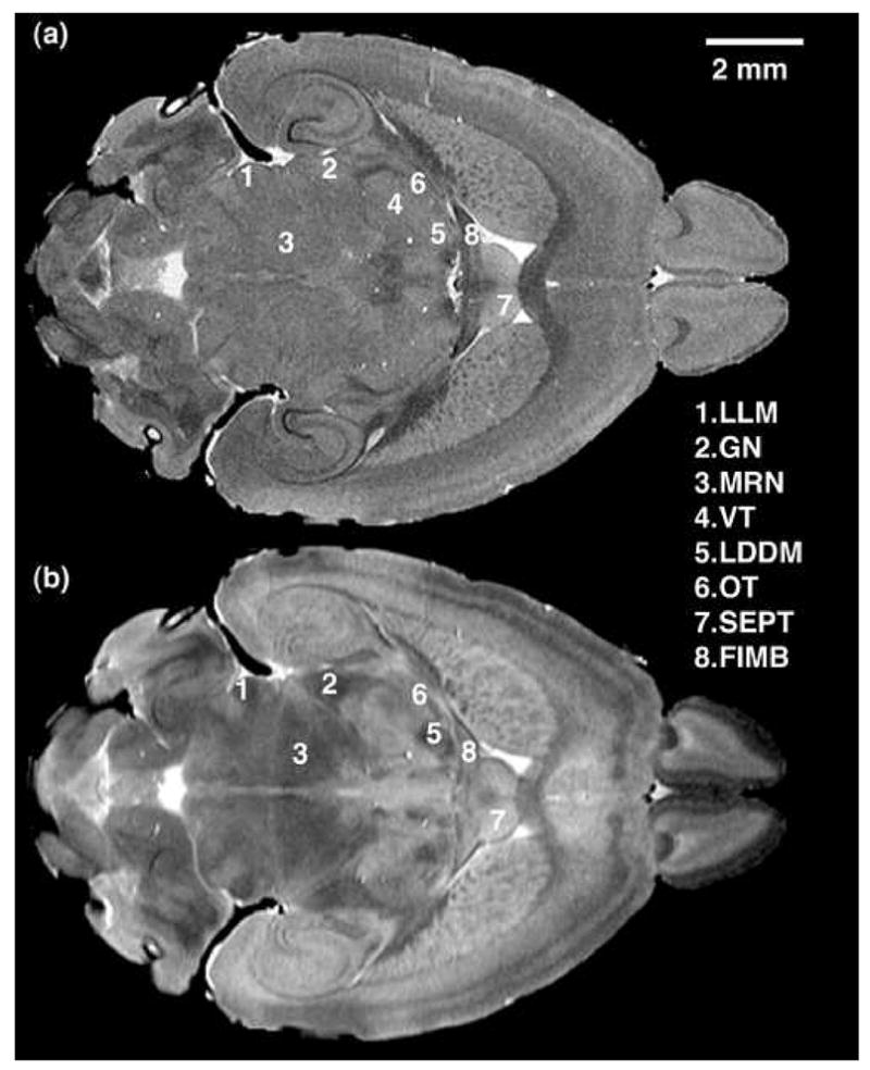
Horizontal slices from (a) T1-weighted and (b) T2-weighted registered acquisitions illustrating different contrast in the two scans for lateral lemniscus (1-LLM), geniculate bodies (2-GN), mesencephalic reticular nucleus (3-MRN), ventral thalamic nuclei (4-VT), laterodorsal thalamic nucleus (5-LDDM), optic tract (6-OT), septal nucleus (7-SEPT), fimbria (8-FIMB).

Segmentation evaluation

The combination of two imaging protocols, the enhanced contrast provided by active staining and MEFIC processing, together with the high resolution of these images allowed the discrimination of 33 structures, including groups of nuclei, white matter tracts, and the ventricular system, as listed in Table 1. .

Fig. 4 shows registered coronal slices from a T1-weighted (a) and MEFIC-T2-weighted (b) data of the brain overlaid transparently with corresponding manual labels (c) and automated segmentation results (d). We evaluated the correspondence between the labels boundaries and the image boundaries, as apparent in the two datasets, as well as the similarity of the labels shapes and their smoothness. A qualitative examination of the segmentations was indicative of the agreement between the two sets of labels, however a quantitative evaluation represents a more accurate assessment of the automated segmentation method.

Figure 4.

Coronal sections through the (a) T1-weighted and (b) T2-weighted datasets, and the manual (c) and automated (d) segmentation results overlaid transparently on the anatomy of the C57BL/6 mouse brain. The color-coding identifies the segmented structures present in the selected coronal slice: corpus calossum (CC), hippocampus (HC), fimbria (FIMB), ventricles (VEN), caudate-putamen (CPU), internal capsule (ICAP), optic tract (OT), amygdala (AMYG), laterodorsal nucleus of the thalamus (LDDM), thalamus (THAL), hypothalamus (HYP), ventral thalamic nulei (VT), globus pallidus (GP).

The measurement of the agreement between the auto-segmented labels and the manual traces was done in two ways: based on the percent voxel overlap and percent volume difference. Fig. 5 illustrates the percent volume overlap between the automated labelings of the 33 segmented structures and their manual tracings, averaged over the brains in the atlas. The graph illustrates the mean percent overlap, together with the standard errors from the mean. The volume overlap is greater than 80% for most structures, except for small irregular or elongated structures, such as the anterior commisure, cerebral peduncles, interpeduncular nucleus, ventricles, and the internal capsule. Even small structures, such as groups of nuclei of the brainstem and thalamus, show high segmentation accuracy: 92.1±0.1% for the mesencephalic reticular nuclei, 86.4±0.1% for the laterodorsal nucleus of thalamus, 84.5±0.1 for ventral thalamic nuclei, 83.8±0.1% for anterior pretectal nucleus, and 81.51±0.02 for geniculate body. The percentage volume difference indicate excellent agreement, with values ranging from 0.8±0.1 % for caudoputamen, 1.4±0.2% for cortex, 1.8±0.3% for brainstem to 10.3±2.6 for the geniculate bodies, 12.7±3.9 for pons, and 13.2±3.7% for trigeminal tract.

Figure 5.

Segmentation validation using the percent voxel overlap (dark gray) and the percent volume difference (light gray) between the automated segmentation results and the manual labels. See Table 2 for abbreviations.

Fig. 6 compares the percent volume overlap results for the high-resolution, high-contrast actively-stained data in this study and the formalin-fixed, comparatively lower resolution data (90 μm) from our previous segmentation efforts (Ali, Dale et al. 2005). The graph indicates that the segmentation of almost all structures is improved in the present study with combined application of active staining, increased resolution, and enhanced T2-weighted contrast. This metric has been computed and compared for structures that were common in the two studies. A two-sample t test with unequal variances was performed for the volume overlap comparing the formalin-fixed brains with the actively-stained brains. Results indicated that for the structures marked with an asterisk in the graph of Fig. 6, the increase in percent volume overlap was statistically significant (p<0.05). Significant improvement is seen in the olfactory bulbs, globus pallidus, caudate putamen, optic tract, anterior commisure, corpus callosum, and ventricles, as well as for brainstem and cortex. Approaching significance (P<0.01) are the improvements in segmentation accuracy for hippocampus and substantia nigra. A smaller, yet distinguishable improvement is noted for most other structures included, with the expection of thalamus and PAG. Improvement in the segmentation of the globus pallidus was directly due to the enhanced contrast and definition in the T2-weighted image. The ventricles in the formalin-fixed excised brain suffered from high variability of shape due to perfusion differences. The actively-stained insitu protocol corrects for this to some extent and could be the cause of improved accuracy in their segmentation. The thalamus shows slightly reduced overlap relative to that seen previously. This could be due to the higher definition of structure now inside the thalamus than in the earlier study where the thalamus was much more homogeneous. The thalamus was subdivided into thalamic nuclei classes, which have a high volume overlap. The other structure segmented with a lesser accuracy is the PAG. However, the difference between the formalin-fixed and actively-stained results was within the standard error of the formalin-fixed results.

Figure 6.

Validation of segmentation based on percent volume overlap between the automated segmentation results and the manual gold standard. The results of automated segmentation for structures segmented in both studies show improvement for the higher resolution, actively-stained images. See Table 2 for abbreviations.

The volumes of the segmented structures have been computed using both the manual and automated labeling, using voxel counting and multiplying the number of voxels by the voxel volume. There was no distinguishable bias in the automatically computed volumes (data not shown).

Fig. 7 compares the segmentation accuracy between the affine registration and the higher order, deformable registration. In general, the results indicated a closer agreement between the manual labels and the automated segmentation based on nonlinear registration, but there is no statistically significant difference compared to the segmentation based on affine registration in the case of the C57BL/6 brains. However, when sizeable volume and shape differences are to be expected, such as in the case of segmenting the brain of a different strain or a genetically modified variant, a nonlinear registration is the method of choice. Therefore, the nonlinear registration method was used in a feasibility study where the segmentation has been applied to a set of BXD mouse brains selected based on the high variability of the hippocampal weight and volumes, as reported by Lu and colleagues (Lu, Airey et al. 2001). A quantitative evaluation has been done only on the known variable structure, the hippocampus, and the agreement between the autosegmented labels and the manual labels ranges from 69.2% for a BXD16 male mouse hippocampus to 82.6% for a BXD 40 male mouse, with an average value of 77.7± 10.8% (Fig. 8). These variations have been obtained for the voxel overlap, while the volume difference between the labeled structures (hippocampi) ranged from 17.6 mm³ for BXD28 to 24.53 mm³ for BXD 16 and 28.4mm³ for BXD40; accounting for a variability up to 34% in the volume of the segmented structures. Fig. 9 illustrates the automatically generated segmentation labels overlaid on the anatomy of the BXD 40 mouse strain.

Figure 7.

Comparison of segmentation accuracy for the C57BL/6J brains based on percent voxel overlap of automated generated labels against manual labels, for the case of affine-based registration and nonlinear registration. The results indicated in general a closer agreement between the manual labels and the automated segmentation when nonlinear registration was used, but the results do not differ significantly compared to segmentation using affine registration.

Figure 8.

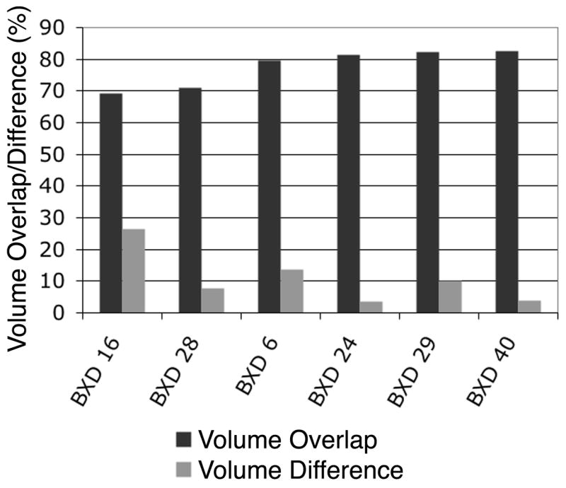
Hippocampus segmentation validation for six recombinant inbred BXD strains. The percent volume overlap averages 78%, while the volume difference averages 11%.

Figure 9.

Segmentation of a BXD 40 mouse brain showing promising results on the applicability of the segmentation method to other mouse strains. (a) Horizontal slices through the T1-weighted (left) and T2 weighted (right) images of the BXD 40 mouse brain. (b) Horizontal slices through the BXD40 mouse brain after its registration to the atlas space. Subtle deformations are noticeable in the shapes of the striatum. (c) Automatically generated labels overlaid on the anatomy of the BXD40 mouse brain in a horizontal (left) and a coronal (right) slice. A qualitative evaluation shows good agreement with the expected labels locations, confirmed quantitatively by the Dice coefficient for the hippocampus.

Discussion

We have shown that the use of multiple contrasts in MR imaging allowed a more comprehensive understanding of the anatomy compared to any single contrast (Ali Sharief and Johnson 2006). The layered structure of the cortex and cerebellum have been identified based on the enhanced contrast of the MEFIC processed T2-weighted images. The increased contrast in this type of images is due to the rapid signal decay of myelin-associated water in cortical layers, which are characterized by short T2s.

Several groups of nuclei located in the thalamus (LDDM, VT, GN) and brainstem (APT, MRN, INFCOL, SUPCOL, PON) have been identified based on the T2-weighted images (see Fig. 2 and Fig. 3). The isolation and volumetric quantification of these nuclei was made possible using the enhanced T2 contrast, while the high-resolution T1-weighted images allowed a better discrimination of hippocampal layers (see granular cell layer in the dentate gyrus [4] in Fig. 2) and thin white matter tracts (see optic tract [6] and fimbria [8] in Fig. 3).

Note that the substantia nigra is hypo-intense in the T2-weighted image and hyper-intense in the T1-weighted image, the internal capsule is clearly demarcated in the T1-weighted image, but the adjoining globus pallidus is not. The T2-weighted image shows the globus pallidus (data not shown). The hypo-intensity of basal ganglia structures substantia nigra and globus pallidus is partly due to deposition of the brain iron ferritin in these regions. This causes magnetic susceptibility differences decreasing tissue T2s and hence a faster decay of signal.

The use of active staining allowed the identification of brain structures with higher detail, such as darkly-stained layers in the hippocampus, white matter striations in the caudate, compared to the formalin-fixed brain. These advantages gained in image contrast also allowed a better qualitative evaluation of the data before manual segmentation.

Together with active staining, higher resolution, and use of multiple contrasts, including the MEFIC processing in the T2-weighted acquisition, enabled the labeling of the mouse brain into a larger number of structure classes and with a higher accuracy than those reported in the formalin-fixed brain (Ali, Dale et al. 2005). The better definition of structures in the current, higher resolution, imaging protocols compared to the unstained data, as well as the fact that the brains were scanned intact in the cranium lead us to believe that the volume estimates in the actively-stained brains are more accurate that those obtained from brains that were scanned after extraction from cranium.

The quantization of morphometic parameters like volumes of the segmented structures makes this method promising for phenotyping the mouse brains. We attempted to segment the brains of mice from 6 BXD strains, for which the hippocampus shows significant variation, as reported by Lu et al. (Lu, Airey et al. 2001), ranging from 21.6 mg on one end of the spectrum to 30.8 mg at the other end of spectrum. This variation in hippocampus weight is reflected in volume differences that can be estimated from MRM segmented images, but also noticeable are differences in the shape of the hippocampus across strains. A global transformation such as an affine registration is not enough to compensate for these changes and a local transformation is required to better match the internal structures of the brain.

A tremendous amount of information regarding the phenome and genome of these BXD mice is available online (see the Mouse Brain Library at http://www.mbl.org/) and it can be expected that volumetric morphometry, as made possible by MR histology, will provide a critical data for connecting specific genetic variations to morphological changes.

The validation of the segmentation method for these six different BXD strains shows promising results (Fig. 8) towards the applicability of this segmentation technique in mouse strains other than the C57BL/6. In the case of the BXD mouse sets, the known genetic background would enable correlating the anatomical phenotype with other phenotypic features, as well as genotype markers. The acquisition and segmentation protocols need to be executed rapidly and the results need to be acquired with a large confidence interval for MRM to become a routine tool for quantitative morphometry. The results here suggest that this will be possible.

References

- Ali AA, Dale AM, et al. Automated segmentation of neuroanatomical structures in multispectral MR microscopy of the mouse brain. Neuroimage. 2005;27(2):425–35. doi: 10.1016/j.neuroimage.2005.04.017. [DOI] [PubMed] [Google Scholar]
- Ali AA, Dale AM, et al. Automated segmentation of neuroanatomical structures in multispectral MR microscopy of the mouse brain. NeuroImage. 2005;27(2):425–435. doi: 10.1016/j.neuroimage.2005.04.017. [DOI] [PubMed] [Google Scholar]
- Ali Sharief A, Johnson GA. Enhanced T2 contrast for MR histology of the mouse brain. Magnetic Resonance in Medicine. 2006;56(4):717–725. doi: 10.1002/mrm.21026. [DOI] [PubMed] [Google Scholar]
- Belknap JK, Phillips TJ, et al. Quantitative trait loci associated with brain weight in the BXD/Ty recombinant inbred mouse strains. Brain Res Bull. 1992;29(3–4):337–44. doi: 10.1016/0361-9230(92)90065-6. [DOI] [PubMed] [Google Scholar]
- Bock NA, Kovacevic N, et al. In vivo magnetic resonance imaging and semiautomated image analysis extend the brain phenotype for cdf/cdf mice. J Neurosci. 2006;26(17):4455–9. doi: 10.1523/JNEUROSCI.5438-05.2006. [DOI] [PMC free article] [PubMed] [Google Scholar]
- Cocosco CA, Zijdenbos AP, et al. A fully automatic and robust brain MRI tissue classification method. Medical Image Analysis. 2003;7(4):513–527. doi: 10.1016/s1361-8415(03)00037-9. [DOI] [PubMed] [Google Scholar]
- Cyr M, Caron MG, et al. Magnetic resonance imaging at microscopic resolution reveals subtle morphological changes in a mouse model of dopaminergic hyperfunction. NeuroImage. 2005;26(1):83–90. doi: 10.1016/j.neuroimage.2005.01.039. [DOI] [PubMed] [Google Scholar]
- Deng HX, Siddique T. Transgenic mouse models and human neurodegenerative disorders. Archives of Neurology. 2000;57(12):1695–1702. doi: 10.1001/archneur.57.12.1695. [DOI] [PubMed] [Google Scholar]
- Fischl B, Salat DH, et al. Whole brain segmentation: automated labeling of neuroanatomical structures in the human brain. Neuron. 2002;33:341–355. doi: 10.1016/s0896-6273(02)00569-x. [DOI] [PubMed] [Google Scholar]
- Fischl B, van der Kouwe A, et al. Automatically parcellating the human cerebral cortex. Cerebral Cortex. 2004;14(1):11–22. doi: 10.1093/cercor/bhg087. [DOI] [PubMed] [Google Scholar]
- Fisher B, Perkins S, et al. Hypermedia Image Processing Reference 1994 [Google Scholar]
- Hashimoto M, Rockenstein E, et al. Transgenic models of alpha-synuclein pathology: past, present, and future. Ann NY Acad Sci. 2003;991(1):171–188. [PubMed] [Google Scholar]
- Iosifescu DV, Shenton ME, et al. An automated registration algorithm for measuring MRI subcortical brain structures. NeuroImage. 1997;6(1):13–25. doi: 10.1006/nimg.1997.0274. [DOI] [PubMed] [Google Scholar]
- Johnson GA, Cofer GP, et al. Morphologic phenotyping with magnetic resonance microscopy: the visible mouse. Radiology. 2002;222(3):789–793. doi: 10.1148/radiol.2223010531. [DOI] [PubMed] [Google Scholar]
- Kapur T, Grimson WEL, et al. Medical Image Computing and Computer-Assisted Interventation —MICCAI’98. Berlin/Heidelberg: Springer; 1998. Enhanced spatial priors for segmentation of magnetic resonance imagery. 1496/1998. [Google Scholar]
- Kovacevic N, Henderson JT, et al. A three-dimensional MRI atlas of the mouse brain with estimates of the average and variability. Cereb Cortex. 2005;15(5):639–45. doi: 10.1093/cercor/bhh165. [DOI] [PubMed] [Google Scholar]
- Lu L, Airey DC, et al. Complex trait analysis of the hippocampus: mapping and biometric analysis of two novel gene loci with specific effects on hippocampal structure in mice. J Neurosci. 2001;21(10):3503–14. doi: 10.1523/JNEUROSCI.21-10-03503.2001. [DOI] [PMC free article] [PubMed] [Google Scholar]
- Ma Y, Hof PR, et al. A three-dimensional digital atlas database of the adult C57BL/6J mouse brain by magnetic resonance microscopy. Neuroscience. 2005;135(4):1203–1215. doi: 10.1016/j.neuroscience.2005.07.014. [DOI] [PubMed] [Google Scholar]
- MacKenzie-Graham A, Jones ES, et al. The informatics of a C57BL/6J mouse brain atlas. Neuroinformatics. 2003;1(4):397–410. doi: 10.1385/NI:1:4:397. [DOI] [PubMed] [Google Scholar]
- Martin MV, Dong H, et al. Independent quantitative trait loci influence ventral and dorsal hippocampal volume in recombinant inbred strains of mice. Genes Brain Behav. 2006;5(8):614–23. doi: 10.1111/j.1601-183X.2006.00215.x. [DOI] [PubMed] [Google Scholar]
- McDaniel B, Sheng H, et al. Tracking brain volume changes in C57BL/6J and ApoE-deficient mice in a model of neurodegeneration: a 5-week longitudinal micro-MRI study. Neuroimage. 2001;14(6):1244–55. doi: 10.1006/nimg.2001.0934. [DOI] [PubMed] [Google Scholar]
- Paxinos G, Franklin KBJ. The Mouse Brain in Stereotaxic Coordinates. New York: Academic Press; 2001. [Google Scholar]
- Peirce JL, Chesler EJ, et al. Genetic architecture of the mouse hippocampus: identification of gene loci with selective regional effects. Genes Brain Behav. 2003;2(4):238–52. doi: 10.1034/j.1601-183x.2003.00030.x. [DOI] [PubMed] [Google Scholar]
- Price DL, Wong PC, et al. The Value of Transgenic Models for the Study of Neurodegenerative Diseases. Ann NY Acad Sci. 2000;920(1):179–191. doi: 10.1111/j.1749-6632.2000.tb06920.x. [DOI] [PubMed] [Google Scholar]
- Rasband W. ImageJ. Bethesda, Maryland, USA: National Institute of Mental Health; 2004. [Google Scholar]
- Redwine JM, Kosofsky B, et al. Dentate Gyrus volume is reduced before onset of plaque formation in PDAPP mice: A magnetic resonance microscopy and stereologic analysis. Proceedings of National Academy of Sciences. 2003;100(3):1381–1386. doi: 10.1073/pnas.242746599. [DOI] [PMC free article] [PubMed] [Google Scholar]
- Rijsbergen CJv. Information Retrieval. London: Butterworths; 1979. [Google Scholar]
- Rueckert D, Frangi AF, et al. Automatic construction of 3-D statistical deformation models of the brain using nonrigid registration. IEEE Trans Med Imaging. 2003;22(8):1014–25. doi: 10.1109/TMI.2003.815865. [DOI] [PubMed] [Google Scholar]
- Wilson JMB, Petrik MS, et al. Quantitative measurement of neurodegeneration in an ALS–PDC model using MR microscopy. NeuroImage. 2004;23(1):336–343. doi: 10.1016/j.neuroimage.2004.05.026. [DOI] [PubMed] [Google Scholar]
- Wong PC, Cai H, et al. Genetically engineered mouse models of neurodegenerative diseases. Nature Neuroscience. 2002;5(7):633–639. doi: 10.1038/nn0702-633. [DOI] [PubMed] [Google Scholar]
- Zavaljevski A, Dhawan AP, et al. Multi-level adaptive segmentation of multi-paramter MR brain images. Computerized Medical Imaging and Graphics. 2000;24:87–98. doi: 10.1016/s0895-6111(99)00042-7. [DOI] [PubMed] [Google Scholar]