Use of a SQUID array to detect T-cells with magnetic nanoparticles in determining transplant rejection

Abstract

Acute rejection in organ transplant is signaled by the proliferation of T-cells that target and kill the donor cells requiring painful biopsies to detect rejection onset. An alternative non-invasive technique is proposed using a multi-channel superconducting quantum interference device (SQUID) magnetometer to detect T-cell lymphocytes in the transplanted organ labeled with magnetic nanoparticles conjugated to antibodies specifically attached to lymphocytic ligand receptors. After a magnetic field pulse, the T-cells produce a decaying magnetic signal with a characteristic time of the order of a second. The extreme sensitivity of this technique, 10⁵ cells, can provide early warning of impending transplant rejection and monitor immune-suppressive chemotherapy.

A methodology using superparamagnetic nanoparticles in conjunction with extremely sensitive magnetometers has been developed to determine if a transplanted organ is undergoing acute rejection by the immune system without requiring biopsies. Rejection of transplanted organs is a significant problem. Transplants replace many different diseased organs such as the kidney, heart, liver and lungs. In kidney disease alone, there are about 52,000 people in the United States on waiting lists for kidney transplants. In addition, 60,000 people die each year of kidney disease. Between 1996 and 1998, 94,000 kidney transplants were done in the United States [1]. One-third of the donors are not good matches. Currently, biopsy is the method to ascertain impending rejection, once the symptoms have occurred, and to monitor the progress of chemotherapy.

Most rejections result from actions of the adaptive immune system. Rejection occurs through several mechanisms including antibodies produced by B-cells, cytokine release, and proliferation of T-cells. The technique described here, focuses on a non-invasive method of detecting, in vivo, T-cell lymphocytes that target and destroy the cells of the transplant, that they recognize as foreign, in the same manner as they destroy true pathogens [2–4]. To offset this response, transplanted organs are selected carefully for compatibility between donor and recipient. The procedure is usually accompanied by chemotherapy designed to minimize the immune system response. This care is often insufficient and the organ is rejected by the recipient. Numerous biopsies may be necessary to monitor progress of the transplanted organ to determine the effect of chemotherapy and success of the transplant. Biopsies, requiring a microscopic examination of the tissue for lymphocytes, delay the diagnosis and thus may miss the early onset of rejection.

Acute rejection can occur within 24 h of transplantation and may persist over days to weeks. The adaptive immune system recognizes certain proteins on the surfaces of cells in the organ as foreign ligands and prepares antibodies to attack these cells. The immune system produces B-cell lymphocytes that generate antibodies that attach to these ligands to label the foreign cells for destruction. The immune system also activates T-cells that can latch onto these foreign cell-surface proteins and kill the transplanted cells. The most important of the proteins distinguishing foreign cells are the major histocompatability complex (MHC) that appears on all invertebrate cells. The MHC proteins in humans are the human-leukocyte-associated antigens (HLA antigens). The presence of proliferating lymphocytes, primarily T-cells, indicates the organ is being rejected. The T-cells recognize the MHC proteins bound to the foreign proteins on the surface of the host cells and they also recognize foreign unattached MHC proteins that may be present in the transplanted tissue [2–4]. The antibodies CD8 and CD4 are co-receptors on T-cells where CD8 is expressed primarily on cytotoxic T-cells recognizing Class I MHC proteins and CD4 is expressed primarily on helper T-cells and Class II MHC proteins.

The large number of lymphocyte cells in the body, approximately 10¹², primarily reside in the lymphatic system and the lymphoid organs (thymus, spleen and appendix). Lymphocytic cells are not normally present in other organs but, on recognition of a foreign substance, exponentially multiply and invade the organ. The patient will suffer fever or other responses to this immune system response. A biopsy of the transplant will be made to determine the presence of lymphocytes through microscopic observation or other means. The initial period of inflammation after the transplant surgery must also be taken into account in any studies of this type. Reduction of biopsies would be of great patient benefit since the biopsies are painful and there is risk of infection, which is of much concern since the patient has a reduced immune system response due to the chemotherapy. Thus any method that can significantly eliminate the need for invasive procedures would have substantial impact on the patient’s well being.

The following discussion outlines the materials and method used in this approach to detecting transplant rejection [5]. This methodology, when used on human beings, is intended to reduce the need for biopsies and to monitor a transplant for the effects of chemotherapy.

(a) Magnetic nanoparticles of 20–25 nm in diameter are conjugated to specific T-cell antibodies, and attached to live cultured T-cells. (b) The cells are inserted into phantoms representing human kidneys and placed under a multichannel superconducting quantum interference device (SQUID) magnetometer [6]. (c) A brief magnetizing field is applied to the cells and particles. (d) The SQUID array detects the decaying remanence fields from these labeled cells after termination of the pulse [5,7]. (d) The field amplitudes are extracted from the data after signal averaging and removal of line-frequency artifacts. (e) A least-squares comparison is done between the field data and a theoretical source representing the known geometry of the sensor array and the total magnetic moment of the cells obtained giving the source strength and location. (f) The moment amplitude is divided by the moment of a single nanoparticle to obtain the total number of nanoparticles in the sample. (g) If the number of cells is known from a cell cytometry measurement, the number of nanoparticles/cell is determined by dividing the number of nanoparticles by the number of cells. (h) If the nanoparticles/cell has been determined previously, the number of cells is determined by this value and the total nanoparticle count. (i) Incubation dependence, saturation effects, and linearity of response are measured using various sample dilutions and incubation times.

The technique requires minute amounts of labeled nanoparticles, consisting of iron oxide, similar to those used as MRI contrast agents and other biomedical applications [7]. These particles would be injected into the subject where they would specifically target activated T-cells. The array of SQUIDs is then used to detect and image the targeted cells. The method is sufficiently sensitive to detect sub-nanograms of iron-oxide material, requiring injected amounts much less than a few milligrams where the known tolerance level is 5 mg/kg of body weight. Results indicate a detection sensitivity of less than 10⁵ live cells at 4 cm from the sensor array. There are similar programs using SQUIDs and remanence field measurements in immunoassay [8] and determination of the parameters of superparamagnetic nanoparticles [9–12].

A photo of one of these cultured T-cells with attached nanoparticles is shown in Fig. 1. The nanoparticles can be seen as points surrounding this cell of approximately 10 μm in diameter. There are about 10,000 nanoparticles attached to this cell.

Fig. 1.

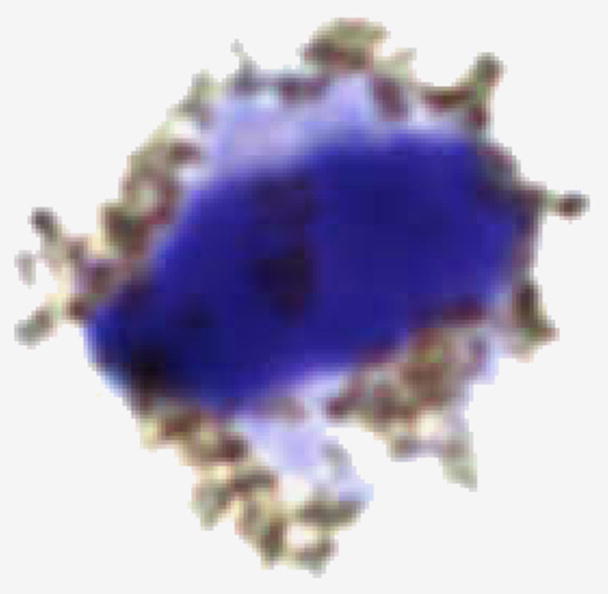
A microscopic photo (20,000 × ), of a live T-cell as used in these measurements. Attached to this cell by CD2 antibodies are approximately 10,000 magnetite nanoparticles of 25 nm diameter with a carboxyl coating.

The nanoparticles that are not bound to cells do not produce measurable fields, eliminating background signals from unbound particles circulating in the blood. This background suppression is a consequence of the two different relaxation times for the alignment of the particle’s permanent magnetic moment following the application of a magnetizing pulse. The first relaxation time, referred to as “Brownian”, applies to particles that are free to rotate in the viscous fluid in which they are suspended. This characteristic time is proportional to the volume of the particle, the viscosity of the suspending solution, and inversely proportional to the temperature. The second relaxation time applies when the physical particle cannot rotate such as, for example, if it were attached to the surface of a cell. In this case, the aligned electron spins comprising the magnetic moment, have to overcome a spin–lattice interaction energy to change their orientations. Even though the single-domain crystal is hindered in its rotation, the collective moment due to the coherent alignment of hundreds of thousands of electron spins does realign. This Néel relaxation time [13] has an exponential dependence on the volume of the magnetic core, the isotropy energy density of the crystal and on the inverse of the absolute temperature. There is also a strong decrease in this time with increasing strength of the applied field.

For magnetite nanoparticles with a core diameter about 24 nm, the Brownian relaxation time is of the order of 1 μs and Néel relaxation time of the order of 1 s. As a result only those particles that are bound to cells are seen by the SQUIDs; the nanoparticles that have not attached to anything will not be seen. Thus, background from the unbound particles is eliminated, unlike the case when such magnetic particles are used as contrast agents in MRI.

Polydispersity leads to important effects. First the particles whose size significantly differs from the optimal will not make any contribution to the signal observed by the SQUIDs. The best sample so far gave only 20% of expected amplitude. One possibility is that ~80% of the binding sites for a T-cell are occupied by particles not producing an observable signal. The signal could be improved by a factor of 5 by simply acquiring the right size distribution if this were the case. However, an alternative explanation for this reduction is that multiple sites are occupied by the same nanoparticle. Also, due to the strong size-dependence of Néel mechanism, particles with even a slight difference in diameter will have noticeably different time constant. As a result the relaxation of the net magnetic moment μ(t) of the nanoparticle ensemble will have non-exponential tail described by

$$\mu (t)=a\hspace{0.17em}ln(1+b/t),$$

where t is the time; a and b can be fit to the data. An exponential fit is used, for the very short times, to extrapolate into t = 0, where the logarithmic relation is singular.

Because the relaxation times predicted by the Néel mechanism decrease drastically for the larger fields that are required to find the asymptotic induced magnetization, the duration of the magnetizing pulse can be fairly short. Normally pulses with 0.3–1 s duration are used, collecting data for 1–10 s after that. To increase the signal-to-background ratio, this pattern is repeated 10–25 times and the obtained signals averaged. A background run with no source is also made to remove the system’s response to the pulsing. Although the pulse is terminated with a field drop to zero in less than 3 ms, a delay of 50 ms is required between the cessation of the magnetizing pulse and the beginning of the measurement period to permit induced currents in the system to die away. The magnetizing pulse from the Helmholtz coils produces a uniform field at the subject of 38 G. Fig. 2 shows these coils located around the snout of the SQUID system, where the pick-up coils are located, positioned above a kidney phantom.

Fig. 2.

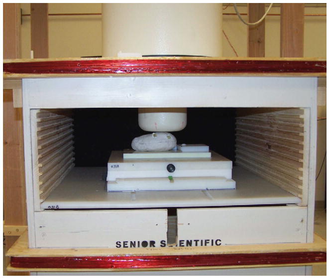
Photo of measurement platform showing SQUID sensors, magnetizing coils, moveable stage and full sized kidney containing two nanoparticle sources of live cells in vials.

In order to determine the number of cells that produce the signal seen by the SQUIDs, the number of nanoparticles bound to each cell must be known, and also the average magnetic moment of the particle. The latter quantity is determined as follows: The average magnetic moment μ_p of the nanoparticles contributing to the signal is obtained by fitting a normalized Langevin function to the “excitation curve” for a given sample. The Langevin function is the average value of the cosine of the angle between the magnetic dipole and the applied magnetic field as determined by classical Boltzmann statistics. The excitation curve is just the signal at a given time t measured by the SQUIDs as a function of the field B produced by the Helmholtz coils, starting at low levels and rising to the maximum possible field. The argument of the Langevin function, i.e. the coupling energy of the dipole to the field divided by the thermal energy, determines the shape of the curve, so by adjusting μ_p the fit can be optimized. Determination of the approximate moment of the particles is necessary in the interpretation of these measurements.

In estimating N, the number of particles contributing to the observed collective dipole moment of the polarized sample, the following representation for the signal measured by the SQUIDs is assumed:

$$S(t,B)=\mu (t)L(x)$$

with x = μ_pB/kT. μ(t) represents the asymptotic limit of the signal (the collective moment of the aligned nanoparticles in the cell cluster) for very large B since L(x) goes to unity. Thus

$$N={lim}_{t\to 0}\mu (t)/{\mu }_p.$$

An exponential fit near t = 0 is used to extrapolate our data to the limit.

The magnetic nanoparticles are Chemicell [Chemicell, Berlin, Germany] Simag-1411 nanoparticles. The iron oxide cores were 25 nm in diameter with 50 nm hydrodynamic radius and provided good remanence field signals. The particles contained a carboxyl coating to provide the linking to the CD2 and CD3 antibodies. The study of the Chemicell particles included measurements of: (1) remanent fields as a function of magnetizing pulse time and amplitude, (2) remanent fields as a function of the medium of deposition—both dried and fluid, and (3) SEM measurements of their diameters. As mentioned above, the core diameter is very important in these measurements in order to obtain the optimal remanence times. An examination of a large variety of nanoparticles from various companies excluded many of their particles because their diameters were either too large or small.

A kidney, as an example of an organ that is typically transplanted, can be simulated using a mold based on a full sized accurate anatomical model. A model using clay was shaped into a kidney phantom. Nanoparticle cluster samples and vials containing liquid and live cells could be inserted into this phantom. These results provided excellent models for the in vitro studies that are necessary to proceed with the in vivo studies in humans.

Fig. 2 displays a kidney phantom under the sensor system with two vials, containing nanoparticles coupled to live T-cells, and inserted at two different positions. Remanence magnetic field distributions from the phantom were obtained by the SQUID array magnetometer to test imaging capabilities for two distinct sources. In addition to vials containing the cells in PBS liquid, small 2–5 mm cotton tips injected with nanoparticles were also inserted into various positions in these phantoms. This phantom method, although quite simple, permits the exploration of the consequences of various nanoparticle types, numbers, bindings, site density of nanoparticles/cell, and cell types using realistic geometries. The kidney phantom was placed under the sensor system to simulate its position in the human body undergoing a biomagnetic scan.

An example of a 7-channel remanence field measurement of live T-cells, SupT1 [14] as placed within the kidney phantom is shown in Fig. 3. SupT1 is an immature continuous T-lymphoblastoid cell line to which the nanoparticles are attached after being conjugated with CD2 antibodies, specific to this line. Both carboxyl- and amino-coated Simag-1411 nanoparticles from Chemicell were used in these experiments. Similar measurements were made on Jurkat cells [15], a human T-cell leukemia line, with nanoparticles labeled with CD3 antibodies. The antibodies are quite specific to these cell lines; Table 1 contains the number of sites for each cell line. Cell cytometry methods [16–18] established the number of antigen sites for the SupT1 cell line displayed for CD2 to be 4.78 × 10⁴ and none for the CD3 antibodies, whereas for the Jurkat cells, there were 3.01 × 10⁴ antigens displayed for the CD3 antibodies and none for the CD2 antibodies. peripheral blood lymphocytes (PBL) were obtained from human serum. They were first labeled with CD2 antibodies and Miltenyi (Miltenyi Biotec Inc., Auburn, CA) nanoparticles and then run through a magnetic separator. The CD2 positive cells were then labeled with CD3 and the Chemicell Simag-1411 nanoparticles. Normal human lymphocyte T-cells have antigens for both CD2 and 3 as the table shows. Approximately 10% of the expected CD3 sites were seen in this experiment. The Miltenyi nanoparticles were too small to produce a measurable signal by this technique. The number of particles bound to each cell is determined by measuring the total magnetic moment from a known number of cells, determined by cytometry count, and dividing the moment by the product of the moment of a single nanoparticle times the number of cells.

Fig. 3.

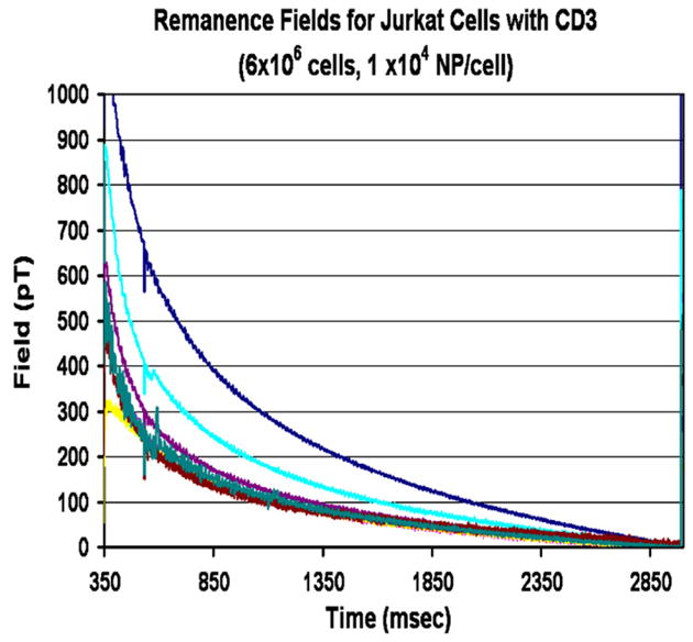
Decaying remanence field as seen in all 7-channel SQUID channels from a source of nanoparticles coupled to Jurkat Cells conjugated with CD3 antibodies.

Table 1.

Prep.	N	Cellsa	Sites/cellb	Sites/cella	% Sites
CD2-SupT1c	5.19 × 1010	5.04 × 106	1.03 × 104	4.78 × 104	22
CD3-Jurkatc	4.16 × 1010	6.72 × 106	6.19 × 103	3.01 × 104	21
CD2-SupT1d	3.35 × 1010	3.72 × 106	9.02 × 103	4.78 × 104	19
CD3-Jurkatd	5.26 × 1010	8.22 × 106	6.40 × 103	3.01 × 104	21
CD3-SupT1	0.0	0.0	0.0	0.0
CD2-Jurkat	0.0	0.0	0.0	0.0
CD2-PBL	5.03 × 104
CD3-PBL	7.30 × 1010	2.22 × 106	3.29 × 104	3.40 × 105	9.7e

^aCytometry count.

^bN/cells.

^cSimag1411(amino).

^dSimag1411(carboxyl).

^eCD2 sites occupied by Miltenyi nanoparticles, CD3 by Simag1411 (amino).

The remanence field measurements were made directly from: (1) vials containing the cells, (2) vials inserted into the phantom, (3) extracted cells placed on small cotton balls inserted into the phantoms, (4) “bare” nanoparticles on cotton balls and (5) “bare” nanoparticles in liquid in the vials. These comparisons served the purpose of extracting net magnetic dipole moments of the cluster and nanoparticles/cell densities. Similarly, the signals from the vials containing the live cells were compared to vials containing “bare” nanoparticles in liquid. The latter gave no measurable signal as expected for unbound particles, confirming that the observed fields were only from particles bound to cells.

These measurements are limited by the current sensitivity of this SQUID system due to noise background of approximately 10 pT. The expected noise limit of the system in a magnetically unshielded environment is 0.04 pT and the dynamic range of the data acquisition system is 0.1 pT so the current noise level is well above instrumental limitations. This noise limits the threshold number-of-cells sensitivity, using the measurement method described above, for T-cells to ~10⁴ at 1 cm and ~10⁵ at 4 cm. These numbers are small compared to the expected number of T-cells accumulating in small nodules in a rejected organ that amount to many millions before symptoms of rejection would occur. There are a number of ways that the current noise floor can be reduced in this system and it is anticipated that a factor of 50–100 increased sensitivity to cells can be achieved.

Imaging measurements made using the 7-channel SQUID system have included single and multiple placements of the stage to simulate either moving the subject under the sensor or moving the sensor above the subject to obtain more complete coverage. The sensors are arranged with one in the center on the axis of symmetry and six in a circle around this at a radius of 2.15 cm, center to center. Initially, the imaging was done with small cotton balls containing nanoparticles described above or vials containing live cells. The ball sources were moved under each of the seven sensors to determine the position of each sensor to 0.02 mm. Cell sources were then placed into the phantoms for imaging following the procedures described above.

Theoretical models of image positions were compared to the remanence field data contained the full geometry of the sensors. The sensors are second-order gradiometers to minimize the contribution of distant background sources. All sources point in the direction of the magnetizing field produced by the Helmholtz coils, the axis of the central sensor.

Fig. 4 is an example of magnetic field contour lines obtained using two vials of live SupT1 cells inserted into the phantom kidney. The vials, in the geometry shown in Fig. 2, and containing nanoparticle and cell counts similar to shown in Table 1, serve as distributed sources. The cells in the vials are suspended in several ml of PBS solution. The contour lines serve as a guide in the x and y value choices in the minimization process. The theoretical and data magnetic field contours are shown side-by-side as obtained by minimizing χ². The results of the fitting procedure for the two sources in the phantom are shown in Table 2 where measured positions of the vials in the phantom are compared to the calculated image fits. The major uncertainty arises from the poorly defined shape of the distributed source represented by the liquid PBS solution in the vial containing the cells. Improvements in the fitting procedure could be obtained using a downhill-simplex method [19].

Fig. 4.

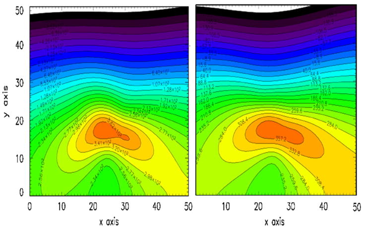
Contour lines of the fields produced by two sources of nanoparticles. On the right are the field contours from the two sources of live cells shown in Fig. 2 and Table 1. On the left are theoretical contour fields from two dipole sources that have been allowed to vary in position and amplitude until a least-squared fit to the data were obtained. The resulting coordinates and source strengths are given in Table 2.

Table 2.

Comparison of source geometries to image results

	x (cm)	y (cm)	z (cm)	m (J pT)
Source 1
Measured	1.4±0.3	−1.1±0.3	5.5±0.3	1.52 × 10−7
Imaged	1.3±0.4	−1.9±0.4	5.0±0.3	1.45 × 10−7
Source 2
Measured	−2.7±0.3	−1.5±0.3	5.5±0.3	1.60 × 10−7
Imaged	−2.7±0.4	−2.2±0.3	5.0±0.3	1.60 × 10−7

^(a)Measurements uncertain due to liquid in vial.

^(b)Imaging errors are SD from fitting.

^(c)Measured m from single vials out of phantom.

To determine the resolution capability of this system using only a single placement of the system, data obtained from a nanoparticle source containing 8.5 × 10⁹ nano particles were fit to the theory. The coordinates, x, y, and z, were varied to obtain values of χ² vs. position for all three axes. These results are shown in Figs. 4 and 5 for a source at a typical distance from sensor to kidney of 4.8 cm. The depth of the source, z, can be determined with a standard deviation of 0.026 cm at a distance of 3–0.20 cm at 5 cm. Extrapolating these findings to deeper sources that might be encountered in human subjects, the depth resolution increases to 0.5 cm at 6 cm from the sensors. Similarly, the x and y resolutions at these distances correspond to standard deviations of 0.25 cm at ~3 cm depth and 0.5 cm at ~5 cm depth. The standard deviation for the collective magnetic moment of 1.82 × 10⁻⁷ J/pT for the last live cell sample of Table 2 is 0.22–10⁻⁷ J/pT. The precision can be improved with additional measurements either through multiple positions in the stage or through the addition of more channels in a larger system. For the imaging case shown in Fig. 5 and Table 2, the SD for value of x1, for example, is improved from 0.50 to 0.43 cm by using two stage positions and could be improved further by additional measurements as previously shown [20].

Fig. 5.

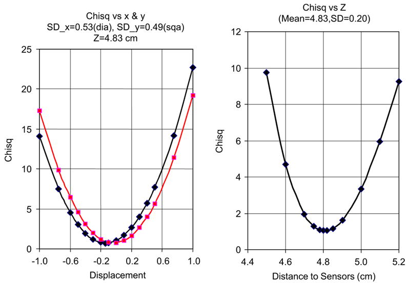
Values of χ² fits to nanoparticle sources as a function of x and y, left figure, and z, the right figure. These were obtained by varying the theoretical forward calculation coordinates and obtaining the χ² values as a function of these coordinates. Standard error analysis were then used to obtain the χ² values.

This study indicates that the biomagnetic approach using labeled nanoparticles to gauge the immune system response to a transplanted organ can be successfully applied to an early diagnosis of impending rejection. The T-cell sensitivity is much greater than other non-invasive techniques and could replace biopsies. The present threshold sensitivity for these cells of ~10⁵ is very small compared to the millions that occur in small nodules in the early stages of immune system attack. Moreover, this high sensitivity could be used to direct drug treatment to counter such attacks while monitoring the amount of T-cells in the transplanted organ. Since no radiation is involved and the quantity of injected iron-oxide nanoparticles is orders of magnitude below tolerance levels, the health of the transplant can easily be repeatedly monitored.

The biomagnetic method for examining the status of a transplant can be applied to many different organs. The kidney has been primarily discussed here because it is the most common organ transplanted. However, this method can also be applied to heart, liver, lung and other transplanted organs as well since the immune system response to transplant is mediated by the T-cells in each case. At present there are only limited animal models to test this methodology although recent work on lung transplants in rats holds promise to alleviate this situation [22–24].

This program complements other areas of SQUID application for the detection of magnetic nanoparticles in biological systems. Extremely sensitive immunoassay studies [8] have been carried out with this technique using SQUID sensors located closely to the samples. A number of pioneering studies in the area of remanence field measurements have produced many of the parameters and formalism for the use of SQUIDs for in vivo studies [9–11]. The present work extends these measurements to live cells and detailed results for nanoparticles coupled to these cells.

References

- 1.Merion RM, et al. JAMA. 2005;294:2726. doi: 10.1001/jama.294.21.2726. [DOI] [PubMed] [Google Scholar]
- 2.Parhan P. Elsevier Ltd; New York/London: 2001. [Google Scholar]
- 3.Bentley GA, Mariuzza RA. Annu Rev Immunol. 1996;14:563. doi: 10.1146/annurev.immunol.14.1.563. [DOI] [PubMed] [Google Scholar]
- 4.McDevitt HO. Annu Rev Immunol. 2000;18:1. doi: 10.1146/annurev.immunol.18.1.1. [DOI] [PubMed] [Google Scholar]
- 5.Flynn ER, Bryant HC. Phys Med Biol. 2005;50:1273. doi: 10.1088/0031-9155/50/6/016. [DOI] [PMC free article] [PubMed] [Google Scholar]
- 6.Hamalainen M, et al. Rev Mod Phys. 1993;65:413. [Google Scholar]
- 7.Andrä W, Nowak H. Magnetism in Medicine. Wiley-VCH; Berlin: 1998. [Google Scholar]
- 8.Chemia Y, Grossman H, Poon Y, et al. Proc Natl Acad Sci. 2000;26:14268. doi: 10.1073/pnas.97.26.14268. [DOI] [PMC free article] [PubMed] [Google Scholar]
- 9.Del Gratta C, et al. In: Aine C, et al., editors. Springer; Berlin: 2000. [Google Scholar]
- 10.Eberbeck D, Hartwig S, Steinhoff U, Trahms L. Magnetohydrodynamics. 2003;39:77. [Google Scholar]
- 11.Eberbeck D, Bergemann Ch, Wiekhorst F, Glöckl G. Magnetohydrodynamics. 2005;41:305. [Google Scholar]
- 12.Pankhurst QA, et al. J Phys D. 2003;36:R167. [Google Scholar]
- 13.Néel L. Ann Géophys. 1949;5:99. [Google Scholar]
- 14.Ablashi DV, et al. J Virol Methods. 1998;73:123. doi: 10.1016/s0166-0934(98)00037-8. [DOI] [PubMed] [Google Scholar]
- 15.Weiss A, Wiskocil RL, Stobo JD. J Immunol. 1984;133:123. [PubMed] [Google Scholar]
- 16.Edwards BS, Curry MS, Tsuji H, et al. J Immunol. 2000;165:404. doi: 10.4049/jimmunol.165.1.404. [DOI] [PubMed] [Google Scholar]
- 17.Larson RS, Brown DC, Sklar LA. Blood. 1997;90:2747. [PubMed] [Google Scholar]
- 18.Larson RS, McCurley TL., III Am J Clin Pathol. 1995;104:204. doi: 10.1093/ajcp/104.2.204. [DOI] [PubMed] [Google Scholar]
- 19.Huang M, Aine CJ, Supek S, et al. Clin Neurophys. 1998;108:32. doi: 10.1016/s0168-5597(97)00091-9. [DOI] [PubMed] [Google Scholar]
- 20.Flynn ER. Rev Sci Instrum. 1994;65:922. [Google Scholar]