A parallel implementation of the Cellular Potts Model for simulation of cell-based morphogenesis

Abstract

The Cellular Potts Model (CPM) has been used in a wide variety of biological simulations. However, most current CPM implementations use a sequential modified Metropolis algorithm which restricts the size of simulations. In this paper we present a parallel CPM algorithm for simulations of morphogenesis, which includes cell–cell adhesion, a cell volume constraint, and cell haptotaxis. The algorithm uses appropriate data structures and checkerboard subgrids for parallelization. Communication and updating algorithms synchronize properties of cells simulated on different processor nodes. Tests show that the parallel algorithm has good scalability, permitting large-scale simulations of cell morphogenesis (10⁷ or more cells) and broadening the scope of CPM applications. The new algorithm satisfies the balance condition, which is sufficient for convergence of the underlying Markov chain.

1. Introduction

Simulations of complex biological phenomena like organ development, wound healing and tumor growth, collectively known as morphogenesis, must handle a wide variety of biological agents, mechanisms and interactions at multiple length scales. The Cellular Potts Model developed by Glazier and Graner (CPM) [1-3] has become a common technique for morphogenesis simulations, because it easily extends to describe the differentiation, growth, death, shape changes and migration of cells and the secretion and absorption of extracellular materials. Some of the many studies using the CPM treat cell–cell adhesion, chicken limb-bud formation and Dictyostelium discoideum development, and non-biological phenomena like liquid flow during foam drainage and foam rheology [4-9].

The CPM approach makes several choices about how to describe cells and their behaviors and interactions. First, it describes cells as spatially extended but internally structureless objects with complex shapes. Second, it describes most cell behaviors and interactions in terms of effective energies and elastic constraints. These first two choices are the core of the CPM approach. Third, it assumes perfect damping and quasi-thermal fluctuations, which together cause the configuration and properties of the cells to evolve continuously to minimize the effective energy, with realistic kinetics, where cells move with velocities proportional to the applied force (the local gradient of the effective energy). Fourth, it discretizes the cells and associated fields onto a lattice. Finally, the classic implementation of the CPM employs a modified Metropolis Monte-Carlo algorithm which chooses update sites randomly and accepts them with a Metropolis–Boltzmann probability.

The Cellular Potts Model (CPM) generalizes the Ising model from statistical mechanics and it shares its core idea of modeling dynamics based on energy minimization under imposed fluctuations. The CPM uses a lattice to describe cells. We associate an integer index to each lattice site (pixel) to identify the space a cell occupies at any instant. The value of the index at a pixel (i, j, k) is l if the site lies in cell l. Domains (i.e. collections of pixels with the same index) represent cells. Thus, we treat a cell as a set of discrete subcomponents that can rearrange to produce cell motion and shape changes. As long as we can describe a process in terms of a real or effective potential energy, we can include it in the CPM framework by adding it to the effective energy. Cells can move up or down gradients of both diffusible chemical signals (i.e. chemotaxis) and insoluble extracellular matrix (ECM) molecules (i.e. haptotaxis). The CPM models chemotaxis and haptotaxis by adding a chemical potential energy, cell growth by changing target volumes of cells, and cell division by a specific reassignment of pixels. If a proposed change in lattice configuration (i.e. a change in the index associated with a pixel) changes the effective energy by ΔE, we accept the change with probability:

$$P\left(\Delta E\right)=\{\begin{array}{cc}1,\hfill & \Delta E\le 0,\hfill \\ e^{-\Delta E∕T},\hfill & \Delta E>0,\hfill \end{array}\phantom{\}}$$ (1)

where T represents the effective cytoskeletal fluctuation amplitude of cells in the simulation in units of energy. One Monte-Carlo Step (MCS) consists of as many index-change attempts as the number of pixels in the lattice (or subgrid in the parallel algorithm). A typical CPM effective energy might contain terms for adhesion, a cell volume constraint and chemotaxis:

$$E=E_{\text{Adhesion}}+E_{\text{Volume}}+E_{\text{Chemical}}.$$ (2)

We discuss each of these terms in Section 2.

Since the typical discretization scale is 2–5 microns per lattice site, CPM simulations of large tissue volumes require large amounts of computer memory. Current practical single-processor sequential simulations can handle about 10⁵ cells. However, a full model of the morphogenesis of a complete organ or an entire embryo would require the simulation of 10⁶–10⁸ cells, or between 10–1000 processor nodes.

Clearly, we need a parallel algorithm which implements the CPM and runs on the High Performance Computing Clusters available in most universities. Wright et al. [14] have implemented a parallel version of the original Potts model of grain growth. However, in this model the effective energy consists only of local grain boundary interactions, so a change of a single pixel changes only the energies of its neighbors. Mombach et al. recently developed a parallel algorithm for the CPM, based on a Random-Walker approach [10]. The standard CPM algorithm always rejects spin flip attempts inside a cell, wasting much calculation time. The Random-Walker approach attempts flips only at cell boundaries, reducing rejection rates. The sequential Random-Walker algorithm runs 5.7 to 15.6 times faster than the standard sequential CPM algorithm depending on the application. However, the parallel scheme in this algorithm depends on a replicated lattice among all processors, which inherently limits its scalability.

We developed a spatial decomposition parallel algorithm based on the common Message Passing Interface Standard (MPI), which allows large scale CPM simulations running on computer clusters. The main difficulty in CPM parallelization is that the effective energy is non-local. Changing one lattice site changes the volume of two cells and hence the energy associated with all pixels in both cells. If a cell's pixels are divided between subdomains located on two nodes and the nodes attempt updates affecting the cell without communication, one node will have stale information about the state of the cell. If we use a simple block parallelization, where each processor calculates a predefined rectangular subdomain of the full lattice, non-locality greatly increases the frequency of interprocessor communication for synchronization and, because of communication latency, the time each processor spends waiting rather than calculating. To solve this problem, we improve the data structure to describe cells and decompose the subdomain assigned to each node into smaller subgrids so that corresponding subgrids on different nodes do not interact, a method known as a checkerboard algorithm. We base our algorithms on those Barkema and collaborators developed for the Ising model, see, e.g., [11]. The checkboard algorithm allows successful parallel implementation of the CPM using MPI [12,13]. Essentially the algorithm uses an asynchronous update algorithm updating different subgrids at different times. When indices on a current subgrid are updated indices on neighboring subgrids are fixed and the cell volume changes occur only on the current subgrid.

In MPI parallelization, the larger the number of computations per pixel update, the smaller the ratio of message passing to computation, and thus the larger the parallel efficiency. In the Ising model, the computational burden per pixel update is small (at most a few floating point operations), which increases the ratio of message passing to computation in a naive partition. However, in the CPM, the ratio of failed update attempts to accepted updates can be very large (typically 10⁴ or more). Only accepted updates change the lattice configuration and potentially stale information in neighboring nodes. The large effective number of computations per update reduces the burden of message passing. However, because we can construct pathological situations which have a high acceptance rate, we need to be careful to check that such situations do not occur in practice.

2. The Cellular Potts Model

In this section we discuss each of energy terms, cell differentiation and reaction–diffusion equations used in the CPM. We also describe the numerical scheme we used in solving reaction–diffusion equations.

2.1. Cell–cell adhesion energy

In Eq. (2)E_Adhesion phenomenologically describes the net adhesion or repulsion between two cell membranes. It is the product of the binding energy per unit area, J_{τ, τ′}, and the area of contact between the two cells. J_{τ, τ′} depends on the specific properties of the interface between the interacting cells:

$$\begin{array}{cc}\hfill E_{\text{Adhesion}}=& \underset{(i,j,k)(i^{\prime },j^{\prime },k^{\prime })\text{neighbors}}{\Sigma }{J}_{\tau \left(\sigma \right){\tau }^{\prime }\left({\sigma }^{\prime }\right)}\hfill \\ \hfill & \times (1-\delta (\sigma (i,j,k),{\sigma }^{\prime }(i^{\prime },j^{\prime },k^{\prime }))),\hfill \end{array}$$ (3)

where the Kronecker delta, δ(σ, σ′) = 0 if σ ≠ σ′ and δ(σ, σ′) = 1 if σ = σ′, ensures that only the surface sites between different cells contribute to the adhesion energy. Adhesive interactions act over a prescribed range around each pixel, usually up to fourth-nearest-neighbors.

2.2. Cell volume and surface area constraints

A cell of type τ has a prescribed target volume v_target(σ, τ) and volume elasticity λ_σ, target surface area s_target (σ, τ) and membrane elasticity ${\lambda }_{\sigma }^{\prime }$. Cell volume and surface area change due to growth and division of cells. E_Volume exacts an energy penalty for deviations of the actual volume from the target volume and of the actual surface area from the target surface area:

$$\begin{array}{cc}\hfill E_{\text{Volume}}=& \underset{\text{All-cells}\sigma }{\Sigma }{\lambda }_{\sigma }{(v(\sigma ,\tau )-v_{\text{target}}(\sigma ,\tau ))}^2\hfill \\ \hfill & +\underset{\text{All-cells}\sigma }{\Sigma }{\lambda }_{\sigma }^{\prime }{(s(\sigma ,\tau )-s_{\text{target}}(\sigma ,\tau ))}^2.\hfill \end{array}$$ (4)

2.3. Chemotaxis and haptotaxis

Cells can move up or down gradients of both diffusible chemical signals (i.e. chemotaxis) and insoluble extracellular matrix (ECM) molecules (i.e. haptotaxis). The energy terms for both chemotaxis and haptotaxis are local, though chemotaxis requires a standard parallel diffusion-equation solver for the diffusing field. The simplest form for chemotactic or haptotactic effective energy is:

$$E_{\text{Chemical}}=\mu \left(\sigma \right)C\left(\overrightarrow{x}\right),$$ (5)

where $C\left(\overrightarrow{x}\right)$ is the local concentration of a particular species of signaling molecule in extracellular space and μ(σ) is the effective chemical potential.

2.4. Cell growth, division and cell death

Typically, we model cell growth by gradually increasing a cell's target volume and cell death by setting the cell's target volume to zero. Cell division occurs when the cell reaches a threshold volume at which point we split the cell into two cells with the same volume, assigning a new index value to one of the new cells.

2.5. Reaction–diffusion (RD) equations

Turing [16] introduced the idea that interactions of two or more reacting and diffusing chemicals could form self-organizing instabilities that provide the basis for spatial biological patterning. We can describe such interactions of reaction and diffusion in terms of a set of reaction–diffusion (RD) equations. The general form for a set of RD equations with M components is:

$$\frac{\partial {\mu }_i}{\partial t}={\nabla }^2{\mu }_i+F_i\left(\mu \right),$$ (6)

where i = 1⋯M, μ = (μ₁⋯μ_M), μ_i is the concentration of the ith chemical species, F_i(μ) is the reaction term.

We use a finite difference numerical scheme to solve the reaction–diffusion equations with calculations being very fast when performed using a sequential algorithm on a small lattice. The chemical field values in the CPM calculations were interpolated from the numerical solution of the reaction–diffusion equations. We plan to parallelize the numerical scheme for the reaction–diffusion equations for larger lattices.

2.6. Cell differentiation

Most multicellular organisms have many different types of cells performing different functions. The cell types result from cell differentiation in which some genes turn on or activate and other genes turn off or inactivate. As a result, different cell types have different behaviors. In the CPM, all cells of a particular differentiation type share a set of parameters describing their behaviors and properties.

3. Data structures and algorithms

3.1. System design principles

Our parallel CPM algorithm tries to observe the following design principles: to implement the CPM model without systematic errors, to homogeneously and automatically distribute calculations and memory usage among all processor nodes for good scalability, and to use object oriented programming and MPI to improve flexibility.

3.2. Spatial decomposition algorithm

Our parallel algorithm homogeneously divides the lattice among all processor nodes, one subdomain per node. The effective energy terms for cell–cell adhesion, haptotaxis and chemotaxis are local, but the constraint energy terms, e.g., for cell volume and surface area, have an interaction range of the diameter of a cell. During a CPM simulation, some cells cross boundaries between nodes. If nodes attempted to update pixels in these cells simultaneously, without passing update information between nodes, cell properties like volume and surface area would stale and energy evaluations would be incorrect. We use a multi-subgrid checkerboard method to solve this problem and Fig. 1 illustrates the topology of the spatial decomposition algorithm. In each node we subdivide the subdomain into four subgrids indexed from 1–4. At any given time during the simulation we restrict calculations in each node to one subgrid with indices at adjacent subgrids being fixed. Notice that each subgrid is much larger than a cell diameter. Therefore, calculation at any given node does not affect the calculations occurring simultaneously at other nodes. Fig. 1 illustrates a cell located at the corner of 4 nodes. If the calculation is taking place at a subgrid of a given node indicated in white, calculations in all other nodes are occurring at white subgrids with no calculations occurring at adjacent subgrids (indicated with different shades of grey). In principle, we should switch subgrids after each pixel update to recover the classical algorithm. Since acceptance rates are low on average, we should be able to make many update attempts before switching between subgrids. However, because acceptance is stochastic, we would need to switch subgrids at different times in different nodes, which is inconvenient. In practice we can update many times per subgrid meaning that sometimes we use stale positional information from the adjacent subgrids. This is possible because the subgrids are large, the acceptance rate is small and the effects of stale positional information just outside the boundaries are fairly weak. We use a pseudo-random switching sequence to switch between sub-grids frequently enough to make the effect of stale positional information negligible compared to the stochastic fluctuations intrinsic to Monte-Carlo methods. Each subdomain hosts a set of buffers which contains pixel information from the border regions of neighboring subgrids. If a flip attempts takes place at a subgrid border, we can retrieve the neighboring subgrid's pixel information from these buffers. Before subgrid switching, the updated subgrid needs to pass this border pixel information to neighboring subgrids.

Fig. 1.

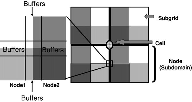
Spatial decomposition. Each computer node consists of four subgrids. At any given time, calculations are performed on only one subgrid of each node indicated in different shading in the figure. Each node includes a set of buffers which duplicate the border areas of neighboring subgrids. During simulations pixel information in neighboring nodes is retrieved from these buffers.

Initialization()SpatialDecomposition()for eachSubRunStepdo CalcuSwitchSequence() for eachsubgrid_runningsdo  for eachupdate_attemptdo   accepted := JudgeUpdate (update)   if (accepted):    CellUpdate()    LatticeUpdate() Communicate() CellMapUpdate() RemapBuffers()if (output) GlobalProperties()Program 1. Algorithm pseudo code.

Program 1 gives the pseudo code for this algorithm. In the pseudo code, Initialization() reads the control file and field information, constructs the framework classes and initializes parameters. SpatialDecomposition() includes topology controller initialization, lattice decomposition, and subgrid initialization. CalcuSwitchSequence() generates a random switching sequence for all nodes. Each SubRunStep lasts a fixed number of MCS. Different instances of SubRunStep can have different switching rates depending on user requirements (we discuss the effect of the switching rate on efficiency in Section 4.2). JudgeUpdate() is a function which determines whether to accept an index change attempt according to Eqs. (1) and (2). CellUpdate() and LatticeUpdate() change the corresponding cell and lattice data for a successful update. Communicate() passes updated lattice and cell information (such as cells' volume and states) to neighboring subgrids and receives corresponding information. CellMapUpdate() allocates memory for incoming cells and updates the CellMap data. RemapBuffers() changes the buffer data from the format in which it is received communicating state (a NodeID and an index ID for each cell) into that used by calculation (pointers to cells).

3.3. Balance condition

The classical Monte Carlo algorithm selects a site or spin at random ensuring that the detailed balance condition is satisfied at all times. In our parallel algorithm detailed balance is violated because the flip cannot be reversed immediately after a subgrid switch. However, detailed balance is unnecessary for the convergence of the underlying Markov chain to be able to converge to the desired equilibrium distribution. Instead, the weaker balance condition is necessary and sufficient for convergence [15].

The Metropolis algorithm evolves a Markov process and generates a sequence of states s₁, s₂, s₃,... with x = (x₁, x₂, x₃,...) as its stationary or equilibrium distribution. We define the transition matrix A(n) (n = 1, 2,....,k) as follows:

$$A_{\mathit{ij}}=q_{\mathit{ij}}{\alpha }_{\mathit{ij}},\forall i\ne j,$$ (7)

$$A_{\mathit{ii}}=1-\underset{i\ne j}{\Sigma }{A}_{\mathit{ij}},$$ (8)

where q_ij is a proposed transitional probability from i to j and α_ij is an acceptance probability from i to j defined as:

$${\alpha }_{\mathit{ij}}=\min \left(1,\frac{x_j}{x_i}\right).$$ (9)

The corresponding transitional kernel (for k sites) of each sweep is the product of all updating matrices

$$P=\prod _{n=1}^k{A}^{\left(n\right)}.$$ (10)

If the parallel algorithm satisfies the balance condition

$${\mathbf{x}}^{\mathrm{T}}\cdot P={\mathbf{x}}^{\mathrm{T}},$$ (11)

the underlying Markov chain converges to the equilibrium distribution.

We now prove that our algorithm satisfies the balance condition. In accordance with the classical Monte Carlo algorithm at every step a site is randomly selected from a lattice. In our parallel algorithm we randomly select a site from the restricted area (inside of a subgrid). However, each single flip of a site or spin is still accepted using Metropolis rules and detailed balance is still satisfied for each A⁽ⁿ⁾

$$x_i{A}_{\mathit{ij}}^{\left(n\right)}=x_j{A}_{\mathit{ji}}^{\left(n\right)},$$ (12)

and thus

$$\underset{i}{\Sigma }{x}_i{A}_{\mathit{ij}}=x_j,$$ (13)

which shows that the balance condition x^T·A⁽ⁿ⁾ = x^T is satisfied for each individual flip of a site or spin. Therefore, we have that

$${\mathbf{x}}^{\mathrm{T}}\cdot P={\mathbf{x}}^{\mathrm{T}}\prod _{n=1}^k{A}^{\left(n\right)}={\mathbf{x}}^{\mathrm{T}}\cdot A^{\left(1\right)}\cdot A^{\left(2\right)}\cdots A^{\left(k\right)}={\mathbf{x}}^{\mathrm{T}},$$ (14)

which proves that the balance condition is still satisfied for each sweep in the parallel algorithm.

3.4. Data structures

The two basic data structures of the parallel CPM algorithm are the cell and the lattice. During simulations, cells move between subdomains which different nodes control. Cells can also appear due to division and disappear due to cell death. In the classical single processor algorithm, each cell has its own global cell index. This data structure works efficiently for sequential algorithms. In a parallel algorithm, this data structure would require a Cell Index Manager to handle cell division, disappearance and hand off between nodes. For example, when a cell divides in a particular node, the node would send a request to the Manager to obtain a new cell index and the Manager would notify all other nodes about the new cell. Instead, we assign each cell two numbers, a node ID and an index ID. The Node ID is the index of the node which generates the cell and the index ID, like the old index, is the index in the cell generation sequence in that node. Since cell IDs are now unique, each node can generate new cells without communicating with other nodes. Since cells may move between nodes, a node dynamically allocates the memory for cell data structures on creation or appearance and releases it when a cell moves out of the node or disappears. To optimize the usage of memory and speed data access, the index in each pixel is a pointer to the cell data structure. Cell properties (such as cell volume, cell area, cell type, center of mass, cell state, etc.) are stored in the data structure “cell map” and when properties of a cell are changed, corresponding data in the cell map is updated. During cell differentiation the corresponding “cell type” value in the cell map structure is updated resulting in the change of cell energy constants. After each subgrid calculation the communication algorithm transfers properties of cells located on subgrids boundaries to adjacent subgrids and synchronizes the adjacent subgrids' cell maps. Fig. 2 illustrates the data structures of the lattice and the cell map.

Fig. 2.

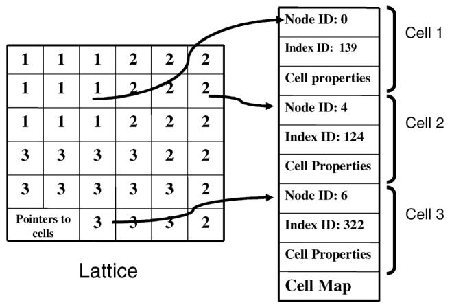
Data structures of the lattice and the cell map. Each cell has a unique cell ID which include a node ID and an index ID. The lattice structure stores pointers to cells.

3.5. Energy calculation

Energy calculation plays an essential role in the CPM. Our parallel algorithm implements three types of energies: adhesion energy, volume energy and chemical energy. Because the local chemical concentration determines the effective chemical energy, this energy is local. Our implementation stores the chemical concentration field in a separate array, which corresponds pixel-by-pixel with the lattice array. The spatial decomposition algorithm we discussed above divides the chemical concentration field into subgrids. Each subgrid contains the chemical field information for energy calculations, so the calculation requires no extra communication. The adhesion energy calculation requires information on the indices in neighboring pixels. Usually, all neighboring pixels lie inside the local subgrid. However, if the pixel is near the subgrid boundary, its neighbors could lie outside the subgrid. In these cases, we retrieve pixel information from the cache buffer arrays which store data from neighboring subgrids (see Fig. 1 and Section 3.2). The width of the buffer depends on the neighbor range of cell–cell adhesion energy calculation demonstrated in Fig. 3. The volume energy has a range of cell diameter and each boundary pixel update changes two cell-volumes. Cell volume and cell area are stored in the cell map structure. During volume energy calculation we retrieve cell volume values from the cell map.

Fig. 3.

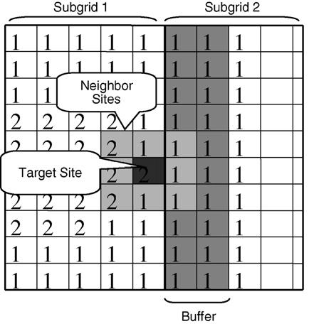
Overlap buffer structure for adhesion energy calculations. Each subgrid can access neighboring subgrid lattices through the overlap cache buffer. We update the overlap cache buffer content after the corresponding subgrid calculation cycle finishes.

3.6. Communication and synchronization

In the spatial decomposition algorithm, when the program switches between different subgrids, the communication algorithm transfers two types of information: lattice configurations and cell information (including cell volumes, cell types and cell states, etc.). In two dimensions, each subgrid needs to communicate with 8 neighboring subgrids (in three dimensions, 26 neighboring subgrids) and the communication algorithm sequentially sends and receives corresponding data according to the spatial organization of the subgrids. Sending and receiving can take place within a node, in which case the algorithm is just a memory copy. Fig. 4 illustrates the communication algorithm. After the communication, the program needs to dynamically update cell maps and overlap buffers. The program also needs to check whether a cell crossed between subgrids and implement the appropriate cell creation or destruction operations.

Fig. 4.

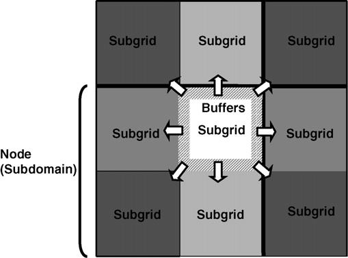
Communication algorithm: After each subgrid calculation cycle, the subgrid needs to transfer data about cells and pixels near its boundary to neighboring subgrids. Lattice sites and associated variables (volume, surface area, etc.) located within the buffer area are transferred so that neighboring subgrids contain correct cell configurations and characteristics.

3.7. Algorithm for treating cells which cross subgrid boundaries

Fig. 5 illustrates the algorithm we employ when a cell crosses a subgrid boundary. When a cell moves into a subgrid, the cell map of the subgrid must allocate memory and issue a temporary cell ID for the cell. Our algorithm does not directly store the Node ID and index ID in the lattice. Instead, each lattice pixel stores a pointer to the corresponding cell and this pointer served as a temporary cell ID to save memory and speed cell property access. When a cell exits a subgrid, the cell map of the subgrid must free the cell's memory and release the cell's temporary ID.

Fig. 5.

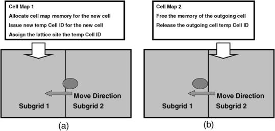
The algorithm for treating cells which cross subgrid boundaries. When a cell crosses a subgrid boundary, the algorithm needs to update cell map values. (a) When a cell moves into a subgrid, the subgrid must allocate the cell map memory and issue a temporary cell ID to the cell, updating the lattice sites and cell map values. (b) When a cell exits a subgrid, the subgrid must free the cell map memory and release the cell's temporary ID.

3.8. Algorithm for global properties calculations

We often wish to track global properties of the configuration, such as the total effective energy, cell topology distribution, etc., for statistical analysis. Global properties are of two types. The first type is pixel related, e.g., chemical energy or adhesion energy. Each subgrid can calculate such statistics by adding values pixel-by-pixel and finally aggregate all information from all nodes (adhesion energy calculations need corrections on sub-grids boundaries). The second type of global properties are cell related, such as volume energy, surface area energy, and volume distributions, etc. Our algorithm stores cell properties (such as volume and surface area) in the cell class and the statistical analysis must calculate these properties cell-by-cell. If each subgrid works independently, cells lying on multiple subgrids will be over counted. In our algorithm, each node sends cell information back to the node to which the cell originally belonged at creation and the creating node then aggregates properties of all cells. Finally node 0 sums up information from each node to obtain correct global properties. Fig. 6 shows details of this algorithm.

Fig. 6.

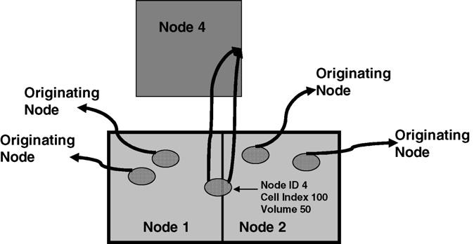
Our algorithm for calculating cell-related global properties (volume energy, volume distribution, etc.). Each node sends cell information (volume, surface area, etc.) back to the node indexed by Node ID which is the node that created the cell. The original creating node then calculates global properties. This algorithm ensures that cell related properties are counted only once when a cell lies in multiple sub-domains.

4. Validation, scalability and discussion

All tests used the Biocomplexity Cluster at the University of Notre Dame. The cluster consists of 64 dual nodes with two AMD 64 bit Opteron 248 CPUs (CPU frequency 2.2 GHz) and 4 GB of RAM each.

We used several special simulations to validate various aspects of our parallel algorithm. Tests checked that boundaries matched between subgrids, that cells responded correctly to different energy terms, and that cells moved correctly between different nodes. Fig. 7 illustrates some of these test results.

Fig. 7.

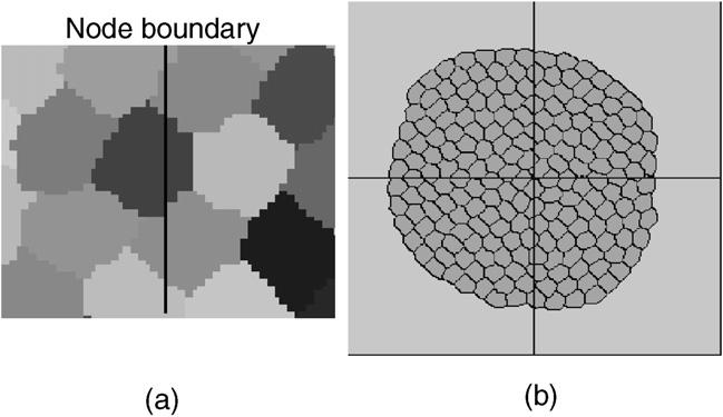
Validation using simple simulations: (a) Cell structures of a node boundary. When cells cross node boundaries, cell boundaries match perfectly between subgrids. (b) A snapshot of a cell coarsening simulation. Cells crossing node boundaries have normal shapes, no cell-boundary discontinuities. The lines indicate the boundaries of the subdomains assigned to each node in a 4 node simulation.

To check how severely stale information affects cells evolution, we used different subgrid switching frequencies to vary the amount of stale information (i.e. a low subgrid switching frequency increases the amount of stale information). We will discuss these results in Section 4.2.

4.1. Scalability of the parallel algorithm

We tested our algorithm for both spatially homogeneous and inhomogeneous configuration of cells. In the latter case, load balance is an important consideration. We use the relative efficiency, normalized by the whole lattice size, to analyze the scalability of our algorithm, defined as: $f=\frac{T_9\times (9∕S_9)}{T_n\times (n∕S_n)}$, where f is the relative efficiency, T_n is the run time of a simulation on a cluster of n nodes, and S_n is the lattice size of the simulation. Since the smallest cluster on which our program runs has 9 nodes, we use the run time on 9 nodes as a reference value.

The first group of performance tests simulate cell coarsening from initially homogeneously distributed cells. Table 1 lists test parameters. Test group (a) used a small size lattice of 300 × 300 per node. Test group (b) used a moderate size lattice of 1000 × 1000 per node. Test group (c) used a large size lattice of 2000 × 2000. Test group (d) checked the effect of subgrid switching frequency on efficiency. Test group (e) distributed the same size lattice on different numbers of nodes. Test (d) has the best scalability because the low switching rate reduces communications. Tests (b) and (c) show almost the same scalability, suggesting that lattice size has a weak effect on scalability. For small lattice sizes (a) the scalability is poor. When the subgrid lattice size is small, preparation for communication (such as socket creation) consumes a significant amount of time. As the lattice size increases, the communication time itself becomes more significant. Test (e) shows good scalability, though worse than that of group (d), because the subgrid lattice size decreases when the number of nodes increases.

Table 1.

Parameters for performance tests on homogeneous patterns

Tests	CPUs	Subgrid switching frequency	Whole lattice size	Cells (106)	Time (sec.)	Relative efficiency
a	9	1/MCS	900 × 900	0.0324	251	1
2000MCS	16		1200 × 1200	0.0576	322	0.779
	25		1500 × 1500	0.09	370	0.678
b	9	1/MCS	3000 × 3000	0.36	254.5	1
200MCS	16		4000 × 4000	0.64	274.5	0.927
	25		5000 × 5000	1	287	0.886
c	9	1/MCS	6000 × 6000	1.44	923.5	1
200MCS	16		8000 × 8000	2.56	975	0.947
	25		10000 × 10000	4	1058.5	0.872
d	9	0.125/MCS	3000 × 3000	0.36	172.5	1
200MCS	16		4000 × 4000	0.64	176.5	0.977
	25		5000 × 5000	1	181.5	0.950
e	9	0.125/MCS	3000 × 3000	0.36	330	1
400 MCS	16				191	0.972
	25				127	0.935

We used a simulation of chondrogenic condensation (see Fig. 15) to test scalability for inhomogeneous cell distributions. Table 2 lists all parameters. Each test ran for 10,000 MCS. For 25 nodes the relative efficiency was 0.89 for this simulation compared to 0.95 for the corresponding homogeneous simulation. The efficiency reduction results from the inhomogeneous cell distribution, which unbalances the load. Fig. 8 shows the load balance for 16 nodes. When a low-load processor finishes a calculation cycle, it must wait until all processors finish their corresponding calculation cycles. The waiting time wastes CPU cycles, which reduces efficiency. The stronger the inhomogeneity the lower the efficiency.

Fig. 15.

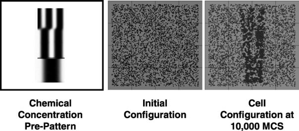
Simulation of chondrogenic condensation during chicken limb-bud formation. The lines indicate the boundaries of the subdomains assigned to each node for a 16-node simulation.

Table 2.

Parameters and results for inhomogeneous pattern tests

Tests	CPUs	Subgrid switching frequency	Whole lattice size	Cells	Time (sec.)	Relative efficiency
1	9	0.125/MCS	1200 × 1200	4500	629	1
2	16		1600 × 1600	8000	653	0.963
3	25		2000 × 2000	12500	707	0.889

Fig. 8.

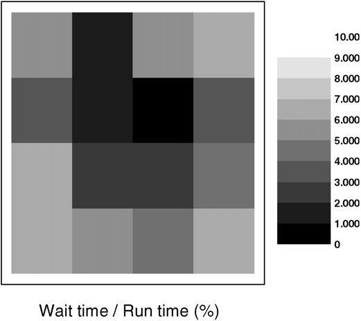
Load balance chart used for the simulation of chondrogenic condensation from Fig. 15. This test uses 16 processors. Each block corresponds to a processor. Grey scale indicates the ratio of waiting time to run time. Dark shows short waiting time and light shows long waiting time.

4.2. Impact of subgrid switching frequency on algorithm performance

In our parallel algorithm, the calculation switches between subgrids after a fixed number of index update attempts and executes the communication subroutine to synchronize lattice and cell information. Frequent subgrid switching reduces efficiency, while infrequent subgrid switching results in cell boundary discontinuities and pattern anisotropy due to stale parameters. We ran tests with different subgrid switching frequencies to analyze the effects of switching rates on efficiencies. and cell patterns. We used a cell coarsening simulation, on a 4000 × 4000 lattice size beginning with 640,000 cells. In the cell coarsening simulation cell boundary motion is solely driven by cell–cell adhesion energy resulting in growths of certain cells, shrinking and disappearance of others. Soap froth is a typical coarsening system [17]. Good agreement between soap froth experiments and the Potts model simulations has been shown in [18]. This simulation used 16 processors and ran for 200 MCS. Subgrid switching frequencies varied from 0.0625 to 8 per MCS. Fig. 9 shows our results. For subgrid switching frequencies higher than once per 4 MCS, the communication time increases substantially and the efficiency decreases. When the subgrid switching frequency is less than 0.25/MCS, the subgrid switching frequency has little effect on the efficiency and real calculations consume more than 80% of the run time.

Fig. 9.

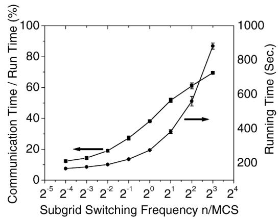
The effect of subgrid switching efficiency on algorithm performance. The lattice size is 4000 × 4000 and the initial number of cells is 640,000.

The above analysis seems to favor low subgrid switching frequencies. However, we must determine whether slow switching rates cause deviations from the cell patterns that the classical algorithm produces. To answer this question, we ran cell sorting tests at low subgrid switching frequencies. The lattice size for this test was 300 × 300 and we ran it on 4 processors. Fig. 10 illustrates the test results. Even for a subgrid switching frequency of 0.0625/MCS (16 MCS per subgrid switch), no significant cell boundary discontinuities occurred at subgrid boundaries.

Fig. 10.

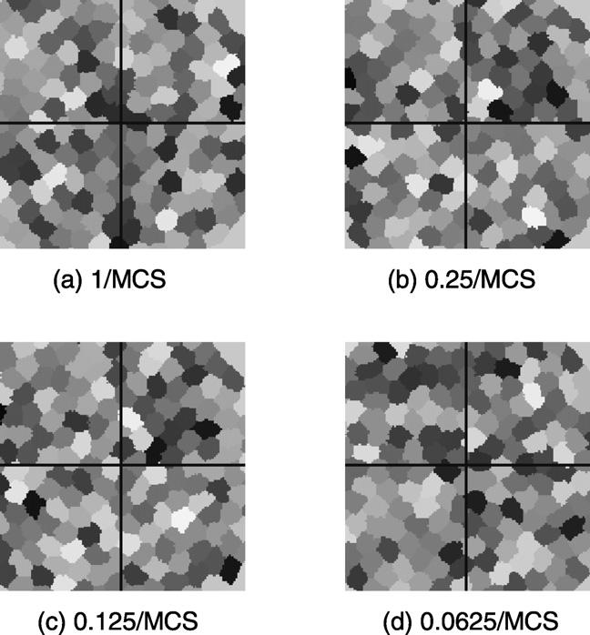
The effect of subgrid switching frequency on a cell sorting simulation with a lattice size of 300 × 300. The grey scale indicates the different cells. Lines indicate the boundaries of the subdomains assigned to each node in a 4-node simulation. The subgrid switching frequency varies from 1/MCS to 0.0625/MCS. No significant cell boundary discontinuity occurs, even for low subgrid switching frequencies (0.125/MCS or 0.0625/MCS).

In the above examples cell volumes stayed near their target values and cell configurations were quite close to equilibrium. However, if configurations were far from equilibrium, energies and configurations would change rapidly and the dynamics of cells at subgrid boundaries could differ from those obtained by using the classical algorithm. We ran several tests of cell growth and haptotaxis with fast dynamics to demonstrate effects of changing subgrid switching frequency on cell patterns.

Fig. 11 illustrates cell growth simulation results. We used 4 processors for each simulation and each simulation contains one cell and medium (ECM). The cell was initially located on the corner of the sub-lattice of one processor (shown in Fig. 11). During simulation the cell crossed node boundaries to other nodes. The initial volume of the cell was 285 and the target volume of the cell was 2000. We ran three simulations with different subgrid switching frequencies (1/MCS, 0.25/MCS and 0.125/MCS). All other test parameters were kept the same: J_1-ECM = 10, volume elasticity λ_σ = 0.11. We ran simulations for a period of 200 MCS on a 300 × 300 lattice. Due to the large difference between the initial and the target cell volume, the volume energy term played the dominant role during the initial stage of the simulation (MCS < 30). Driven by the volume energy, the cell growth was a very fast dynamic process at this stage and the adhesion energy term was too weak to maintain the smooth cell boundary. For subgrid switching frequency of 1/MCS and 0.25/MCS no significant cell boundary discontinuities occurred at subgrid boundaries. For subgrid switching frequency of 0.125/MCS and MCS = 8 the cell did not cross the node boundary because subgrid switching was performed only once during this time. No significant cell boundary discontinuities occurred at subgrid boundaries with MCS = 24 and MCS = 200. Fig. 12 demonstrates good agreement between simulations of cell growth dynamics (cell volume vs. MCS number) obtained for different subgrid switching frequencies, using parallel CPM and sequential CPM. Averaged results of 5 test runs are shown. Parallel algorithm yields correct dynamics even at the initial stage of the process (MCS < 30) with switching frequency of 0.125/MCS, which corresponds to fast dynamics.

Fig. 11.

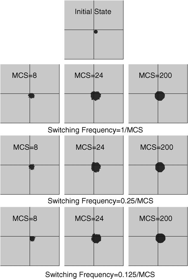
The effect of subgrid switching frequency on cell growth simulations with a lattice size of 300×300. Lines indicate the boundaries of the subdomains assigned to each node in a 4-node simulation. The subgrid switching frequency varies from 1/MCS to 0.125/MCS and for each switching frequency cell configurations of MCS = 8, MCS = 24 and MCS = 200 are illustrated.

Fig. 12.

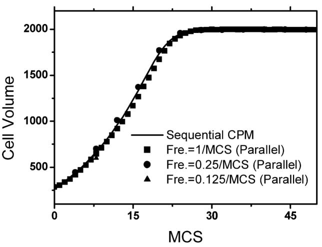
The effect of subgrid switching frequency on cell growth dynamics. The subgrid switching frequency varies from 1/MCS to 0.125/MCS for the parallel algorithm. For the comparison purpose we also illustrate the sequential CPM result. We performed 5 separate tests for each curve and show the average of the values. Energy parameters and initial configurations used in tests are the same as those of Fig. 11.

Fig. 13 illustrates simulation results of the haptotaxis process. In this test we used 4 processors for each simulation containing one cell and medium (ECM) with initial simulation configuration shown in Fig. 13 and chemical concentration C(x, y) = x + y. We ran three simulations with different subgrid switching frequencies (1/MCS, 0.25/MCS and 0.125/MCS) and with a large effective chemical potential value 300.0. All other test parameters were kept the same: J_1-ECM = 5, volume elasticity λ_σ = 0.1. Simulations ran for 200 MCS on a 300 × 300 lattice. Driven by the chemical energy, the cell moved from the lower right node to the upper left node. Due to the large chemical energy potential value (μ = 300.0) the shape of the moving cell was irregular. For subgrid switching frequency of 1/MCS and 0.25/MCS, no significant cell boundary discontinuities occurred at subgrid boundaries. For subgrid switching frequency of 0.125/MCS, the cell did not move into upper nodes with MCS = 16 since subgrid switching was performed only twice during this time. No significant cell boundary discontinuities occurred at subgrid boundaries for MCS = 40.

Fig. 13.

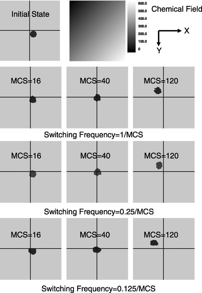
The effect of subgrid switching frequency on haptotaxis simulations with a lattice size of 300 × 300. Lines indicate the boundaries of the subdomains assigned to each node in a 4-node simulation. The subgrid switching frequency varies from 1/MCS to 0.125/MCS and for each switching frequency cell configurations of MCS = 16, MCS = 40 and MCS = 120 are illustrated.

In both fast dynamic processes simulations using the parallel algorithm give good results, especially with sub-grid switching frequencies of 1/MCS and 4/MCS. In practice systems usually have slower dynamics and in such a case stale-information effects are weaker.

We also tested the scalability and efficiency for larger scale fast dynamic processes using cell growth and haptotactic processes as test examples. The cell growth test involved only one cell type and the cell target volume value (ν_target = 2000) was much bigger than the initial cell volume value (ν_target = 285). Each node contained 400 cells on a 1000 × 1000 lattice to ensure enough space being available for cell growth. Cells were randomly distributed on the lattice. Parameters were chosen as follows: J_1-ECM = 10, volume elasticity λ_σ = 0.11, sub-grid switching frequency = 0.25/MCS. Each simulation ran for 200 MCS. The haptotaxis simulation involved one cell type with and the cell target volume value (ν_target = 285) was the same as the initial cell volume value (ν_target = 285). J_1-ECM = 5, volume elasticity λ_σ = 0.1, chemical potential μ = 300.0, chemical field C(x, y) = x + y, sub-grid switching frequency = 0.25/MCS, each simulation ran for 200 MCS. Testing results listed in Tables 3 and 4 demonstrate good efficiency of the parallel algorithm for fast dynamic processes. For example, on 25 processors cluster with sub-grid switching frequency = 0.25/MCS the relative efficiencies of cell growth simulation and haptotactic simulation are 0.906 and 0.910, respectively.

Table 3.

Parameters and results for cell growth tests

Tests	CPUs	Subgrid switching frequency	Whole lattice size	Cells	Time (sec.)	Relative efficiency
1	9	0.250/MCS	3000 × 3000	3600	107	1
2	16		4000 × 4000	6400	112	0.955
3	25		5000 × 5000	10000	118	0.906

Table 4.

Parameters and results for haptotaxis tests

Tests	CPUs	Subgrid switching frequency	Whole lattice size	Cells	Time (sec.)	Relative efficiency
1	9	0.250/MCS	3000 × 3000	3600	102	1
2	16		4000 × 4000	6400	108	0.944
3	25		5000 × 5000	10000	112	0.910

The communication speed of the cluster plays an important role in algorithm efficiency. Users of our algorithm should calibrate their cluster by running subgrid switching frequency tests on short simulations and choose subgrid switching frequencies to balance efficiency and stale-information effects.

4.3. Morphogenesis simulations

Steinberg's Differential Adhesion Hypothesis (DAH), states that cells adhere to each other with different strengths depending on their types [19,20]. Cell sorting results from random motions of the cells that allow them to minimize their adhesion energy, analogous to surface-tension-driven phase separation of immiscible liquids [19]. If cells of the same type adhere more strongly, they gradually cluster together, with less adhesive cells surrounding the more adhesive ones. Based on the physics of the DAH, we model cell-sorting phenomena as variations in cell-specific adhesivity at the cell level. Fig. 14 shows two simulation results for different adhesivities. All other parameters and the initial configurations of the two simulations are the same. In simulation (a), cell type 1 has higher adhesion energy with itself (is less cohesive) than cell type 2 is with itself. The heterotypic (type 1–type 2) adhesivity is intermediate. During the simulation, cells of type 2 cluster together and are surrounded by cells of type 1. In simulation (b), the adhesivity of cell type 1 with itself is the same as the adhesivity of cell type 2 with itself and greater than the heterotypic adhesivity. This energy hierarchy results in partial sorting.

Fig. 14.

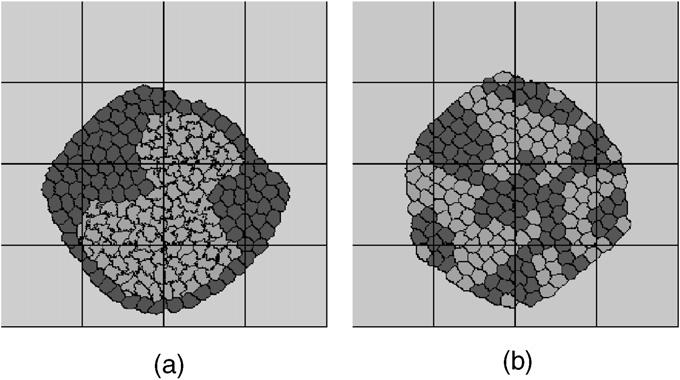
Cell sorting simulation. Cell type 1 (dark). Cell type 2 (light). Extra cellular matrix (ECM) (grey). The two simulations use the same initial cell configuration and target volumes (ν_target = 150), the only differences between (a) and (b) are the different adhesion constants. (a) Adhesion constants: J₁₋₁ = 14, J₂₋₂ = 2, J₁₋₂ = 11, J_1,2-ECM = 16. (b) Adhesion constants: J₁₋₁ = 14, J₂₋₂ = 14, J₁₋₂ = 16, J_1,2-ECM = 16. The lines indicate the boundaries of the subdomains assigned to each node in a 16-node simulation.

During development of the embryonic chick limb, the formation of the skeletal pattern depends on complex dynamics involving several growth factors and cell differentiation. Hentschel et al. have developed a model of the precartilage condensation phase of skeletogenesis based on reaction diffusion and interactions between eight components: FGF concentration, four cell types, TGF-β concentration (activator), inhibitor concentration, and fibronectin density [21]. The mechanism leads to patterning roughly consistent with experiments.

Fig. 15 shows a simulation of Hentschel-type chondrogenic condensation run on 16 nodes with a total lattice size of 1200 × 1200. This simulation used an externally-supplied chemical pre-pattern to control cell differentiation and cell condensation.

4.4. Discussion

The main tradeoff in using the new asynchronous update algorithm is accuracy—potentially affected by use of stale information—vs. parallel efficiency. The right parameters to use depend on the type of kinetic process modeled, as well as the speed of the computing and network facilities. Provided the accuracy of the model is acceptable, the algorithm converges to the desired equilibrium distribution, since it satisfies the balance condition. Future work will address optimization of the communication and load balance schemes.

Our parallel algorithm uses the classic Monte-Carlo site updating algorithm which wastes computer time by selecting and then rejecting non-boundary sites which cannot be updated. Combining our parallel algorithm with an algorithm which selects only boundary sites like the Random Walker algorithm [10] will greatly improve efficiency. Long communication times, especially with high subgrid switching frequencies, also reduce efficiency. The current algorithm transfers the entire contents of the overlap buffers during the communication phase, which is wasteful. Optimizing the communication step by sending and receiving only updated sites will save communication time and increase efficiency.

One problem with our fixed-boundary spatial decomposition is load imbalance for spatially heterogeneous simulations. One possible solution is to use smaller subgrids and assign multiple low-load subgrids to single processors. However, this method requires additional communication time to transfer lattice and cell information between processors. Alternatively we could dynamically move node boundaries to decrease load imbalance. This method would require a complex topology manager to monitor load balance and dynamically manipulate node boundary positions.

5. Conclusion

Most implementations of the widely-used CPM are sequential, which limits the size of morphogenesis simulations. Our parallel algorithm uses checkboard domain decomposition to permit large-scale morphogenesis simulations (10⁷ cells or more). It greatly broadens the range of potential CPM applications. Our initial tests on cell coarsening, cell sorting and chicken limb bud formation show good scalability and ability to reproduce the results of single processor algorithms.

References

- 1.Graner F, Glazier JA. Simulation of biological cell sorting using a two dimensional extended Potts model. Phys. Rev. Lett. 1992;69:2013–2016. doi: 10.1103/PhysRevLett.69.2013. [DOI] [PubMed] [Google Scholar]
- 2.Glazier JA, Graner F. Simulation of the differential adhesion driven rearrangement of biological cells. Phys. Rev. E. 1993;47:2128–2154. doi: 10.1103/physreve.47.2128. [DOI] [PubMed] [Google Scholar]
- 3.Weaire D, Glazier JA. Relation between volume, number of faces and three-dimensional growth laws in coarsening cellular patterns. Phil. Mag. Lett. 1993;68:363–365. [Google Scholar]
- 4.Chaturvedi R, Huang C, Izaguirre JA, Newman SA, Glazier JA, Alber MS. On multiscale approaches to three-dimensional modeling of morphogenesis. J. R. Soc. Interface. 2005;2:237–253. doi: 10.1098/rsif.2005.0033. [DOI] [PMC free article] [PubMed] [Google Scholar]
- 5.Cickovski T, Huang C, Chaturvedi R, Glimm T, Hentschel HGE, Alber MS, Glazier JA, Newman SA, Izaguirre JA. A framework for three dimensional simulation of Morphogenesis. IEEE/ACM Trans. Comp. Biol. Bioinform. 2005;3:1545–1566. doi: 10.1109/TCBB.2005.46. [DOI] [PubMed] [Google Scholar]
- 6.Mombach J, Glazier JA. Single cell motion in aggregates of embryonic cells. Phys. Rev. Lett. 1996;76:3032–3035. doi: 10.1103/PhysRevLett.76.3032. [DOI] [PubMed] [Google Scholar]
- 7.Marée AFM. From pattern formation to morphogenesis. Utrecht University; Netherlands: 2000. PhD thesis. [Google Scholar]
- 8.Jiang Y, Glazier JA. Foam drainage: Extended large-Q Potts model simulation. Phil. Mag. Lett. 1996;74:119–128. [Google Scholar]
- 9.Jiang Y, Swart P, Saxena A, Asipauskas JA. Glazier, hysteresis and avalanches in two dimensional foam rheology simulations. Phys. Rev. E. 1999;59:5819–5832. doi: 10.1103/physreve.59.5819. [DOI] [PubMed] [Google Scholar]
- 10.Mombach JCM, Cercato FP, Cavalheiro GH. An efficient parallel algorithm to evolve simulations of the cellular Potts model, Parallel Process. Lett. 2005;15:199–208. [Google Scholar]
- 11.Barkema GT, MacFarland T. Parallel simulation of the Ising model. Phys. Rev. E. 1994;50:1623–1628. doi: 10.1103/physreve.50.1623. [DOI] [PubMed] [Google Scholar]
- 12.Gropp W, Lusk E, Skjellum A. Using MPI: Portable Parallel Programming with the Message Passing Interface. second ed. MIT Press; Cambridge, MA: 1999. [Google Scholar]
- 13.Gropp W, Lusk E, Thakur R. Using MPI-2: Advanced Features of the Message-Passing Interface. MIT Press; Cambridge, MA: 1999. [Google Scholar]
- 14.Wright SA, Plimpton SJ, Swiler TP, Fye RM, Young MF, Holm EA. Potts-model grain growth simulations: Parallel algorithms and applications. SAND Report. 1997 August;:1925. [Google Scholar]
- 15.Manousiouthakis VI, Deem MW. Strict detailed balance is unnecessary in Monte Carlo simulation. J. Chem. Phys. 1999;110:2753–2756. [Google Scholar]
- 16.Turing AM. The Chemical Basis of Morphogenesis. Philos. Trans. R. Soc. B (London) 1952;237:37–72. [Google Scholar]
- 17.Stavans J, Glazier JA. Soap froth revisited: Dynamical scaling in the two dimensional froth. Phys. Rev. Lett. 1989;62:1318. doi: 10.1103/PhysRevLett.62.1318. [DOI] [PubMed] [Google Scholar]
- 18.Glazier JA, Anderson MP, Grest GS. Coarsening in the two-dimensional soap froth and the large-Q Potts model: A detailed comparison. Phil. Mag. B. 1990;62:615. [Google Scholar]
- 19.Davis GS, Phillips HM, Steinberg MS. Germ-layer surface tensions and tissue affinities in Rana pipiens gastrulae: Quantitative measurements. Dev. Biol. 1997;192:630–644. doi: 10.1006/dbio.1997.8741. [DOI] [PubMed] [Google Scholar]
- 20.Beysens DA, Forgacs G, Glazier JA. Cell sorting is analogous to phase ordering in fluids. Proc. Natl. Acad. Sci. (USA) 2000;97:9467–9471. doi: 10.1073/pnas.97.17.9467. [DOI] [PMC free article] [PubMed] [Google Scholar]
- 21.Hentschel HGE, Glimm T, Glazier JA, Newman SA. Dynamical mechanisms for skeletal pattern formation in the vertebrate limb. Proc. R. Soc. Lond: Biol. Sci. 2004;271:1713–1722. doi: 10.1098/rspb.2004.2772. [DOI] [PMC free article] [PubMed] [Google Scholar]