Mechanoenzymes under superstall and large assisting loads reveal structural features

Abstract

Single-molecule experiments on the motor protein kinesin have observed runs of backsteps and thus a negative, that is, reverse mean velocity, V, under superstall loads, F; but, counterintuitively, beyond stall, V(F) displays a shallow minimum and then decreases in magnitude. Conversely, under assisting loads V(F) rises to a maximum before decreasing monotonically. By contrast, while the velocity of myosin V also saturates under assisting loads, the motor moves backward increasingly rapidly under superstall loads. For both kinesin and myosin V this behavior is implied remarkably well by simple two-state kinetic models when extrapolated to large loads. To understand the origins of such results in general mechanoenzymes, biochemical kinetic descriptions are discussed on the basis of a free-energy landscape picture. It transpires that the large-load performance is determined by the geometrical placement of the intermediate mechanochemical states of the enzymatic cycles relative to the associated transition states. Explicit criteria are presented for N-state sequential kinetics, including side-reaction chains, etc., and for parallel-pathway models. Physical colocalization of biochemically distinct states generally implies large-load velocity saturation.

Single-molecule studies of motor proteins and other mechanoenzymes (1–4) under varying imposed loads aim to uncover features of the underlying biochemical structure and mechanisms. Thus, in recent experiments (5, 6) on conventional kinesin, a highly processive motor, the mean velocity, V, along the microtubule track (which we will suppose is aligned with the positive x axis) has been measured, at various concentrations of ATP, as a function of an imposed load F = (F_x, F_y, F_z) in both resisting and assisting regimes. [Sideways and oblique loads have also been examined (5, 7).]

Observed Behavior and Large-Load Extrapolations

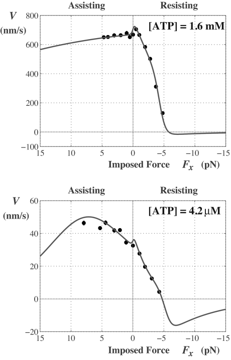
Fig. 1 displays the data of Block and coworkers (5) as the x component of F varies (with F_y = 0). In the resisting regime, F_x < 0, shown on the right, the observations extend up to a stall force of F_S ≃ −(6–7) pN at which, by definition, the velocity vanishes. The assisting regime, F_x > 0, extends on the left to F_x ≃ +8 pN. Remarkably, “helping the motor” by pulling it in the positive (or “designed”) direction, results in a decreasing velocity at high [ATP]. At low [ATP] the assistance does at first increase the speed; but then V appears to reach a relatively low maximum. This unexpected behavior is well captured by the solid curves, which represent a theoretical fit (8, 9) that recognizes the vectorial character of the load F transmitted to the motor body. The fit at low [ATP] suggests that V(F_x) would also decrease quite rapidly at larger loads.

Fig. 1.

Velocity vs. x component of the load F for kinesin. The data, for [ATP] = 1.6 nm and 4.2 μM are from Block et al. (5) and the fits to a two-state kinetic model embodying a free-energy landscape picture are from Fisher and Kim (8).

Perhaps more surprising is the behavior predicted by the extensions of the fitted plots into the superstall regime where the resistive load |F_x| exceeds |F_S|. Then, the velocity changes sign and becomes negative, corresponding to a reverse or backstepping motion. However, the speed remains small, 10–30 nm/s; furthermore, some 20–30% beyond F_S the plots undergo shallow minima, and thereafter, V(F_x) approaches zero from below.

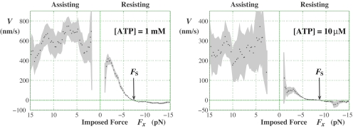
These predictions were not reported originally (8) and, indeed, might well be regarded as merely representing an unwarranted extrapolation of theory into a totally new domain of motor operation (10). Nevertheless, as seen in Fig. 2, when Carter and Cross (6) explored this highly resisting superstall regime just such low, 10–40 nm/s, backward velocities emerged. Furthermore, unambiguous minima appeared, albeit at somewhat higher loads. What might be the implications of this seemingly anomalous behavior?

Fig. 2.

Velocity vs. load for kinesin derived from observations of Carter and Cross (6). Detailed data for the fractions of forward and backward steps, π₊ and π₋, and corresponding dwell times, τ, as functions of a running (1.5 pN)-bin averaged force yield the velocity via V = d(π₊ − π₋)/τ (11, 12), where d = 8.2 nm represents the kinesin step size. The gray shading indicates the confidence intervals based on the number of observations.

The Carter–Cross data in Fig. 2 for assisting (F_x > 0) loads also confirm the conclusions from Block et al. (5) regarding the decrease of V at high [ATP]: despite the noise, a clear drop-off is seen for F_x ≳ 5 pN. Similarly, at [ATP] = 10 μM, a relatively small rise is followed by a downward trend not inconsistent with the anomalous decay at larger forces implied by the 4.2 μM fit in Fig. 1.

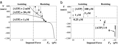
Comparable velocity vs. load data for myosin V derived from observations by Mehta et al. (13) under resistive loading up to the stall force F_S ≃ −2.8 pN are shown in Fig. 3a. The original substall fits to these data (14) have been extrapolated analytically to both the assisting and large resisting (F_x < F_S) regimes (see Fig. 3a). For superstall loads, the fits closely merge, indicating an independence of [ATP]; then, in contrast to kinesin, the predicted velocity plunges rapidly to negative values exceeding 800 nm/s. For assisting loads, however, the implied behavior more closely reflects that for kinesin: the fits exhibit broad maxima that, ultimately, decrease to zero (although this is not evident graphically for high [ATP]).

Fig. 3.

Myosin V. (a) Substall data derived from Mehta et al. (13) fitted to a two-state kinetic model by Kolomeisky and Fisher (14) (evaluated here also for [ATP] = 20 μM). Note the factor of 2 scale change for negative, superstall velocities. (b) The velocity under superstall and large assisting loads [after Gebhardt et al. (15)]. The solid symbols represent data for [ATP] = 1 μM; those for F_x = −(5 and 10) pN have been narrowed and displaced slightly to distinguish data for [ATP] = 0, 0.25 μM up to 0.1 mM. Note the scale change for V < −200 nm/s.

Experiments by Gephardt et al. (15) ranging from F_x = 10 pN to −10 pN, serve to check these expectations. As evident from Fig. 3b, the extrapolated substall fits provide a remarkable (and even semiquantitative) description of the striking fall of V(F_x) to large backward values. Note, especially, the observed independence of [ATP] beyond stall. Furthermore, the assisting-load measurements confirm the predicted saturation effect: for [ATP] = 1 μM, there is little increase above V(0); while for 100 μM, even the anomalous decrease with increasing F_x seems confirmed.

In summary, in addition to seeking the origins of the large-load behavior of kinesin, one should ask why myosin V is so different in the superstall regime. More generally, how is it that simple two-state kinetic models, matching only data for low loads, extrapolate so successfully to both large assisting and resisting loads?

Free-Energy Landscape and Transition States

To make progress, consider the basic N-state kinetic model (4, 8, 9, 14) in which a mechanoenzyme in an initial or waiting state [0] binds a substrate molecule (e.g., ATP) and proceeds forward through a succession of N mechanochemical states (j = 1, 2, …), completing a cycle by reaching the final state [N] that, biochemically, is identical to [0], while mechanically the enzyme has completed a forward “step”: for a rotary motor (2, 3), this step could be an angular increment, Δθ; but for a translocatory motor on a track (the situation on which we will focus), it will be a linear displacement, d x̂ [where x̂ is a unit vector and d is close to 8.2 nm for kinesin and 36 nm for myosin V (1, 2)]. Chemical reversibility demands that, for each forward transition from state (j) to (j+1) at a rate u_j, there is a reverse transition from (j+1) to (j) with a (nonvanishing) rate w_j+1.

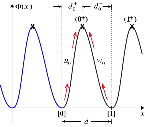
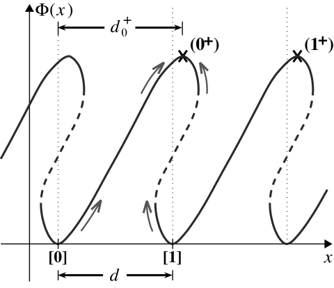
To account for imposed loads one needs expressions for u_i(F) and w_i(F); these follow from a free-energy landscape picture (1, 4, 8, 9, 16, 17). The most primitive example, an (N = 1) model with just two rates, u₀ and w₀, is illustrated in Fig. 4. Here, the coordinate x locates the enzyme, a motor protein, as it moves on the periodic track. A free-energy barrier generates a transition state, marked by a cross, which must be overcome by thermal activation when the motor moves either forward or backward. As depicted, Φ(x) is periodic which implies no net forward drift: this corresponds to stall, that is, V = 0 and F = F_S = (F_S, 0, 0).

Fig. 4.

The simplest one-dimensional free-energy landscape, Φ(x), where the coordinate x represents the point of attachment P on the motor at which the load force F = (F_x, 0, 0) is imposed. The transition states (0⁺) and (1⁺) are marked by crosses. Note that states [0] and [1] are biochemically equivalent although physically displaced; likewise, (0⁺) and (1⁺).

However, on imposing a force F (≠F_S) the free-energy function becomes Φ(x) ⇒ Φ(r)−(F−F_S)·r, where, for generality, we have identified a “point of attachment,” P[r = (x, y, z)], on the body of the motor. Thus, a substall force tilts the landscape potential downward lowering the barrier for a forward transition and, hence, increasing u₀ while the reverse transition rate, w₀, is reduced.

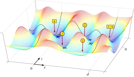
In general, as illustrated in Fig. 5, the landscape Φ(r) will be more complex and depend also on the z and y coordinates of P. Potential wells (or valleys) at locations r_j correspond to intermediate states (j). Reaction paths between neighboring states, (j) and (j + 1), traverse cols (or passes or saddles) that determine the associated transition states at r_j⁺ = r_{j + 1}⁻ (see, e.g., ref. 9). To leading exponential order in F, traditional reaction-rate theory then yields (1, 8, 9)

where the “partial substeps” are given by

and obey Σ_j(d_j⁺ + d_j⁻) = d (see, e.g., Fig. 4). The θ_j^± are “load distribution vectors” or, neglecting the y and z components, “load distribution factors,” θ_j^±; they clearly sum to unity (4, 8, 9).

Fig. 5.

An (N = 3)-state free-energy landscape, Φ(r), with locally stable intermediate states (j) for j = 0, 1, 2, …, labeled and with an extra “side state” (2′). The neglect of the transverse y coordinate is justified if Φ increases rapidly with y². The transition states, at r_j⁺ = r_{j + 1}⁻, are marked by crosses. If the pass between state (2′) and [3 ≡ 0] becomes sufficiently high, the (2′, 3) transitions will be suppressed: then a (1, 2′) transition represents a side reaction off the main reaction path [0] ⇌ (1) ⇌ (2) ⇌ [3] (see Figs. 8 and 9).

Velocities under Large Loads for N = 1

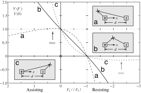
In the following we will appeal to formulas for V in terms of the set of 2N transition rates {u_j(F), w_j(F)} (see, e.g., ref. 18). To gain insight, however, let us initially neglect F_y and F_z and consider only the simplest case N = 1 for which V/d = u₀(F) − w₀(F). For the situation in Fig. 4 one may reasonably regard x as a reaction coordinate so that the transition state lies, physically, between states [0] and [1] and 0 < θ₀⁺ ≡ d₀⁺/d < 1. Then one finds (see curve b in Fig. 6) that superstall loads necessarily lead to large negative speeds, that is, formally, V(F_x) → −∞ as F_x → −∞, while assisting loads lead to the complementary behavior, that is, V(F_x) → +∞ as F_x → +∞. Thus, the expected or “normal” performance under large loads is mandatory in both regimes. Conversely, the unnatural or “anomalous” response seen in Figs. 1–3 (minima and decreasing reverse speeds at superstall and saturation/maxima for assisting force) cannot be captured!

Fig. 6.

Variation of velocity with imposed force for the (N = 1)-state model with, as specific examples, u₀⁰/w₀⁰ = 4 and load distribution factors: (a) θ₀⁺ = −0.2, (b) θ₀⁺ = 0.4, and (c) θ₀⁺ = 1.2; as depicted in Insets a, b, and c. Cases b and c correspond to Figs. 4 and 7. Recall, as in Fig. 4, that states [0] and [1] are biochemically equivalent.

It is crucial to realize, however, that the physical displacement x of the point of attachment, P, need not be an acceptable reaction coordinate. Indeed, the “minimal” adequate biophysiochemical or enzymatic structural space may entail the y and z coordinates of P and other “unseen” dimensions (8, 9, 16, 17). Thus, as illustrated in Fig. 7, the transition state may lie outside the natural domain 0 < x < d. There are two new cases: first, if, as in Figs. 6c and 7, one has θ₀⁺ = d₀⁺/d > 1, then, necessarily, anomalous superstall behavior is generated. See plot c in Fig. 6; formally, we can assert: V(F_x) → 0⁻ when F_x → −∞. Nevertheless, only normal behavior is realized under assisting loads: plots b and c in Fig. 6.

Fig. 7.

A one-dimensional landscape, as in Fig. 4, but with a transition state displaced so that θ₀⁺ = d₀⁺/d > 1. Various portions of the plot should be regarded as projected from other physical or chemical dimensions (so that the free-energy Φ remains single-valued as a function of an appropriate reaction coordinate).

In the last case, θ₀⁺ = d₀⁺/d is negative, and superstall variation must be normal but assisting-load anomalous behavior arises, that is, V(F_x) → 0 when F_x → +∞ (see Fig. 6a).

In all cases, the qualitative large-load behavior is independent of the specific values of the load-free rates, u₀⁰ and w₀⁰. In other words, the performance under superstall and assisting loads is determined only by structural features of the landscape Φ(x). Is that true more generally? If so, what are the crucial features? And when are both superstall and assisting-load behavior anomalous?

N-State Sequential Motor Protein Models

Recall, now, that N-state sequential models are specified by 2N rates {u_i, w_j} and 2N structural parameters, namely, {r_j, r_j⁺}, the state and transition state locations of the attachment point, P. Fig. 8 portrays two complete cycles of an N = 3 system. Note that states (j) and (j ± N) and (j⁺) and (j⁺ ± N) are biochemically identical, although physically distinct; the corresponding periodicity conventions r_j+kN = r_j + kd x̂ and r_j+kN^± = r_j^± + kd x̂, for k = ±1, ±2, …, are embodied in the figure.

Fig. 8.

Two cycles of an (N = 3)-state sequential model corresponding to Fig. 5 projected on to the (x, z) plane but neglecting state (2′). The locations of states (j) and transition states (j⁺) are displayed along with N² = 9 significant structural vectors, r_i+j⁺ − r_i, for i = 0, 1, 2, that is, (r₀⁺ − r₀), (r₁⁺ − r₀), (r₂⁺ − r₀), (r₁⁺ − r₁), etc. Recall that states [0], [3], and [6] are biochemically equivalent, as are states (1) and (4), (2) and (5), etc.

To account for the vectorial nature of the force F, we follow refs. 8 and 9, noting that the tether transmitting force to the motor body in a typical single-molecule bead assay (1, 4–7) is inclined, say at a polar angle θ to the z axis. Hence, the experimentally controlled component F_x induces a normal component F_z ∝ |F_x| (8, 9). (We suppose F_y ≡ 0.) Although the orientation of the tether switches fairly abruptly (8, 9) when the load changes from resisting to assisting, the magnitude of θ, mainly fixed by the bead diameter (8, 9), can be taken as constant. Consequently, in using Eq. 1 we may suppose

where c_‖ = cot θ > 0. [For kinesin one has c_‖ ≃ 1.45 (9).]

Now, by employing known theory (18), one may write the turnover rate, or reduced velocity, in the form (12)

where the N² force-independent inverse rate parameters K_i,j are nonvanishing, positive ratios of various products of the zero-load rate constants {u_k⁰, w_l⁰}. However, the force dependence for F_x ≷ 0 is controlled by the 2N² key geometrical parameters

for i, j = 0, 1, …, N − 1. These may be regarded as projections on to c⁺ and c⁻ (for F_x ≷ 0) of the vectorial substeps from a state r_i to the transition state r_i+j⁺. See, for example, the nine vectors from states [0], (1), and (2) in Fig. 8 given by j = 0, 1, and 2.

Now the way is clear! When large superstall loads are tested (formally, F_x → −∞), Eq. 4 yields |V| ≈ exp[|F_x|(d − D_max⁻)/k_BT], where D_max⁻ is the largest projection D_i,j⁻. Consequently, we can conclude, in words:

A: Anomalous superstall variation, V → 0⁻, results if but only if at least one of the N² projections D_i,j⁻ exceeds the step size d.

Note that this justifies the conclusion illustrated in Fig. 6c. Inspection of Fig. 8, however, reveals that the landscape of Fig. 5 [without state (2′)] cannot yield anomalous superstall behavior but could do so if the coordinate x₁ became smaller than x₀⁺.

The complementary argument for F_x > 0 applied to Eq. 4 (formally, F_x → +∞) clearly yields:

B: Assisting-load anomalous behavior, V decreasing, is realized if but only if at least one of the N² projections D_i,j⁺ is negative.

This bears out the convex form of Fig. 6a but shows that only normal assisting load performance is realizable for the system in Fig. 8. Furthermore, when N = 1 there is only one term in the denominator in Eq. 4; thus, an anomalous response for both signs of F_x is forbidden unless N ⩾ 2. Conversely, as demonstrated by Fig. 1 (8), two-state models can be doubly anomalous.

Colocalization and Fuel Dependence

The structural projections in Eq. 5 are expressible by using the load distribution vectors, θ_i⁺ and θ_j⁻ (see Eq. 2). Thus, in Fig. 8, one has D_j,0⁺ = c⁺·θ_j⁺d, D_j,1⁺ = c⁺·(θ_j⁺ + θ_j+1⁻ + θ_j+1⁺)d, etc., and, using the periodicity, for example,

and so on. Now it may happen that to a good approximation a transition state, say (j⁺) or (j⁻), and an adjacent biochemically distinct state, say (j), are physically colocalized so that θ_j⁺ = (r_j⁺ − r_j)/d or θ_j⁻ = (r_j − r_j⁻)/d vanishes. Thus, real biochemical changes, (j − 1) ⇌ (j⁻) ⇌ (j) ⇌ (j⁺) ⇌ (j + 1), occur, but the point of attachment, P(x, y, z), on the motor undergoes no appreciable displacement in the step (j) ⇌ (j⁺) or in the step (j⁻) ⇌ (j) [although, of course, (j⁺) or (j⁻) will likely differ from (j) in significant but unseen dimensions]. The corresponding vanishing of D_j,0⁺ then implies, by Eq. 4 and B, that under large assisting loads V(F_x) will saturate, that is, approach a maximal value.

Similarly, under resisting forces, the associated equality D_j,N−1⁻ = d that follows from Eq. 6, takes one to the borderline at which anomalous superstall behavior sets in (see A). Accordingly, the backward velocity is then expected to decelerate as |F_x| increases above F_S and approach a limiting or minimal negative value.

In application of kinetic models to motor proteins, the supply of molecular fuel or substrate, say ATP, is well represented by taking u₀⁰ = k₀⁰[ATP] as the initial, zero-load rate; the stall force can then be set by a corresponding form for the reverse rate w₀⁰ (or w_N−1⁰, etc.) (see refs. 4, 8, 14, and 19). The dependence or otherwise of the large-load velocity on the fuel supply, as noted in connection with myosin V in Fig. 3, hinges, therefore, on the inverse rate parameters K_i,j in Eq. 4. When |F_x| → ∞, one of the N² terms in the denominator will dominate exponentially and carry a corresponding inverse rate, say K⁻ or K⁺ for F_x ≷ 0. If these particular parameters do not depend on [ATP], that is, do not carry u₀⁰ as a factor [or, possibly, w₀⁰, etc. (14, 19)], the large load response will be independent of [ATP], and vice versa. For a given landscape this can be checked from expressions for K_i,j (12).

Side-Reaction Paths

Experiments on RNA polymerase (20) have observed “pauses” in otherwise steady stepping along the DNA track. Such intermittent motions suggest the presence of reaction side chains that branch off the main pathway (see Fig. 9). The previous theory is readily generalized for side-reaction chains (and trees, etc.) (12, 18). If a sequence of L states, located, say, at r_k^s for k = 1, 2, …, L, springs from state (s) at r_S ≡ r₀^s, one needs 2NL further structural parameters to extend conclusions A and B: these are the vector projections

and each is associated with an inverse rate parameter K_j,k^s as in Eq. 4, but entailing also the side-reaction zero-load transition rates {u_k−1⁰, w_k⁰} (12). For the example in Fig. 9 the corresponding LN = 1 × 3 new vectors have been drawn in.

Fig. 9.

Two cycles of the three-state model in Fig. 8 augmented by a side-reaction path of length L = 1 branching from state (1) to state (2′) yielding three additional significant structural vectors.

Both anomaly assertions A and B now remain valid provided that one supplements “the N² projections D_i,j⁻” (or “D_i,j⁺,” respectively) by “and the LN projections D_{j,k s}⁻” (or “D_{j,k s}⁺”). Application to the side-reaction system of Fig. 9, where the vector (r₁⁺−r_2′) has a relatively large negative x component, reveals a surprise: whenever c_‖ is not too large, the assisting-load (V, F_x) profile will be anomalous (even though a normal superstall response remains).

If there are a number of side paths, one need only include the extra vector projections in the anomaly condition list (12).

Parallel Pathway Mechanoenzymes.

Various lines of evidence (4) suggest a need for models with alternative pathways to achieve cycle completion. In the simplest case, two independent parallel pathways of N_α and N_β transitions run from the unique state [0] via (1_α) or (1_β) to (N_α − 1) or (N_β − 1) and meet again at [N_α] ≡ [N_β]. Kolomeisky (21) has obtained exact results for V that can be recast (and extended to multiple parallel pathways) as a sum of two terms, V_α + V_β, each with (by appeal to detailed balance) the same numerator as in Eq. 4. The denominators are distinct but coupled together (12). Then 2(N_α² + N_β²) structural parameters, D_i,j^α± and D_l,m^β±, can be defined in precise analogy to Eq. 5; these suffice to determine the large-load behavior.

Because the two chains are linked at state [0], it proves essential to distinguish the corresponding projections, D_0,j^α± and D_0,m^β±, from those with roots at i, l ≠ 0. Then we may introduce N_αβ ≡ N_αN_β(N_β − 1) “coupled projections” by

where j, m ⩾ 0 while l ⩾ 1. The N_βα N_βN_α(N_α − 1) parameters D_m;i,j^βα− are defined similarly (with i ⩾ 1), while for the complementary N_αβ-coupled projections, D_j;l,m^αβ+ and D_m;i,j^βα+, min replaces max. Finally, the first anomaly condition can be stated as: A^‖ Anomalous superstall variation is realized if but only if, first, at least one of the (N_α² + N_αβ) α-projections, D_i,j^α− and D_j;l,m^αβ−, and, second, at least one of the (N_β² + N_βα) β-projections, D_l,m^β− and D_m;i,j^βα−, exceeds the step size d.

The complementary condition B^‖ for assisting load anomalies follows merely by replacing each superscript minus sign in A^‖ with a plus sign and changing the final phrase to “is negative.”

These parallel pathway criteria for anomalous behavior seem more demanding than for two distinct single chains. Nevertheless, the coupling actually provides extra possibilities beyond the single-chain requirements. To see this, suppose N_α = N_β = 2 and, for simplicity, consider c_‖ = 0 so that only the scalar load distribution sets, Θ_α ≡ (θ_α0⁺,θ_α1⁻,θ_α1⁺,θ_α0⁻) and Θ_β, are needed to specify the α- and β-chain structures. The concrete assignments

which verify Σ_jθ_λj^± = 1, then prove instructive.

By way of Eq. 5, these yield the sets {D_i,j^α±} and {D_l,m^β±} of N_α² + N_β² = 4 basic structural projections for each chain, namely,

where i, j, l, m = 0, 1. Consider first each chain individually: from the criteria A and B one sees that the α-chain cannot display anomalous (V, F_x) profiles. Since D_11β^± > d, however, the β-chain will be anomalous above stall: this is a consequence of the negative load factor θ_β1⁻, as is easily seen in a plot like Fig. 8.

But when the two chains are coupled we must appeal to A^‖ and use Eq. 1 to compute the N_αβ = 4 coupled projections, noting first from Eq. 10, that max_n(D_0,n^β−) = 0.7d whence one finds

Since D_1;1,1^αβ exceeds d we conclude that the coupled (α,β) chains will, in fact, jointly exhibit anomalous superstall behavior. Lastly, it should be remarked that side reactions branching off one or both pathways can be handled analytically just as explained above for the sequential models (12). Explicit analytical results have also been found (12) for looped side reactions in which a transition sequence of M ⩾ 2 steps branches off from a particular state to which it returns on the last step. However, the possible role of such “isolated futile cycles” is not presently clear.

Discussion

Our analysis of the conditions under which large loads lead to anomalous (V, F_x) responses might well be explored for other enzyme schemes. Most pressing perhaps are divided pathway systems, in which, after N_γ (>1) steps, the enzyme can proceed by two distinct routes, say α and β, that meet again with N_δ (⩾0) steps remaining before the full cycle is completed. Fig. 5 represents a (1, 2, 2, 0) example. There is, indeed, evidence that myosin V has such a significant alternative pathway (22, 23). A closed formulation for V(F_x) in terms of all of the 2Σ_λ N_λ rates has been derived (12). On using that, explicit criteria emerge regarding the large-load behavior, but they lack the intuitive clarity and relative simplicity exemplified in the anomaly rules A, B, A^‖, and B^‖ derived above. Specifically, disconnected four–state vector differences, such as (r_i⁺ − r_j + r_k⁺ − r_l), appear and must also be used.

Rather than describe a systematic algorithm for still more complex kinetic models (12) let us reflect briefly on the results obtained. Foremost is the fact that mechanoenzyme performance under large imposed forces is determined by a relatively few general parameters that physically locate specific transition states relative to intermediate biomechanochemical states.

Furthermore, as already demonstrated for kinesin (8), allowance for motions of the enzyme normal to the track, or, generally, in the full (x, y, z) space, may be crucially important. Likewise significant is the recognition, illustrated in Figs. 6 and 7, that a mechanochemical transition state need not lie “physically” between the biophysical states it links. This recognizes that the obvious physical coordinate measuring the progress of a mechanoenzyme may not be a satisfactory reaction coordinate: thus, as in Figs. 6 and 7, “local backtracking” may occur even though the enzymatic transitions move steadily forward (11).

Recall next, the observations in Figs. 1–3 demonstrating that reverse motions and their fuel dependence under superstall loads can be successfully predicted by simple kinetic models and smoothly linked to substall performance without invoking further mechanisms. These facts bring into question various proposals (e.g., refs. 10 and 15), arguing that new effects and special phenomena should enter when, under the imposition of a large resistive load, a mechanoenzyme progresses backward. Although novel features could play a role when a mechanoenzyme is reversed by overload, one might, in the absence of contrary evidence, rather hold that the fundamental biophysiochemical picture of a series of reactions being reversed merely by tilting the free-energy landscape, that is, altering the balance of free energy, should be accepted as the primary hypothesis.

Finally, when an imposed force is switched from resisting or opposing, as usually considered normal for mechanoenzymes, to assisting or helping, it is certainly reasonable to allow for specific mechanical changes; merely reversing the sign of F_x in a formula fitted for F_x < 0 is unlikely to prove adequate. In our analysis this was recognized explicitly by introducing in Eq. 3 the projection vectors c^± that allow for the tether orientation. But, in a detailed analysis of kinesin (8), a further specific mechanism was invoked on the basis of the experimental data (7). Nevertheless, the paramount role of the geometrical location of states and transition states should remain under large assisting forces just as in the superstall regime.

References

- 1.Howard J. Mechanics of Motor Proteins and the Cytoskeleton. Sunderland, MA: Sinauer; 2001. [Google Scholar]
- 2.Schliwa M, editor. Molecular Motors. Weinheim: Wiley–VCH; 2003. [Google Scholar]
- 3.Berg HC. Annu Rev Biochem. 2003;72:19–54. doi: 10.1146/annurev.biochem.72.121801.161737. [DOI] [PubMed] [Google Scholar]
- 4.Kolomeisky AB, Fisher ME. Annu Rev Phys Chem. 2007;58:675–695. doi: 10.1146/annurev.physchem.58.032806.104532. and references therein. [DOI] [PubMed] [Google Scholar]
- 5.Block SM, Asbury CL, Shaevitz JW, Lang MJ. Proc Natl Acad Sci USA. 2003;100:2351–2356. doi: 10.1073/pnas.0436709100. [DOI] [PMC free article] [PubMed] [Google Scholar]
- 6.Carter NJ, Cross RA. Nature. 2005;435:308–312. doi: 10.1038/nature03528. [DOI] [PubMed] [Google Scholar]
- 7.Lang MJ, Asbury CL, Shaevitz JW, Block SM. Biophys J. 2002;83:491–501. doi: 10.1016/S0006-3495(02)75185-0. [DOI] [PMC free article] [PubMed] [Google Scholar]
- 8.Fisher ME, Kim YC. Proc Natl Acad Sci USA. 2005;102:16209–16214. doi: 10.1073/pnas.0507802102. [DOI] [PMC free article] [PubMed] [Google Scholar]
- 9.Kim YC, Fisher ME. J Phys Condens Matter. 2005;17:S3821–S3838. doi: 10.1088/0953-8984/17/47/013. [DOI] [PubMed] [Google Scholar]
- 10.Molloy JE, Schmitz S. Nature. 2005;435:286–287. doi: 10.1038/435285a. [DOI] [PubMed] [Google Scholar]
- 11.Tsygankov D, Lindén M, Fisher ME. Phys Rev E. 2007;75:1–16. doi: 10.1103/PhysRevE.75.021909. 021909. [DOI] [PubMed] [Google Scholar]
- 12.Tsygankov D, Fisher ME. J Chem Phys. 2007 doi: 10.1063/1.2803213. [DOI] [PubMed] [Google Scholar]
- 13.Mehta AD, Rock RS, Rief M, Spudich JA, Mooseker MS, Cheney E. Nature. 1999;400:590–593. doi: 10.1038/23072. [DOI] [PubMed] [Google Scholar]
- 14.Kolomeisky AB, Fisher ME. Biophys J. 2003;84:1642–1650. doi: 10.1016/S0006-3495(03)74973-X. [DOI] [PMC free article] [PubMed] [Google Scholar]
- 15.Gebhardt JCM, Clemen AE-M, Jaud J, Rief M. Proc Natl Acad Sci USA. 2006;103:8680–8685. doi: 10.1073/pnas.0510191103. [DOI] [PMC free article] [PubMed] [Google Scholar]
- 16.Keller D, Bustamante C. Biophys J. 2000;78:541–556. doi: 10.1016/S0006-3495(00)76615-X. [DOI] [PMC free article] [PubMed] [Google Scholar]
- 17.Xing J, Wang H, Oster G. Biophys J. 2005;89:1551–1563. doi: 10.1529/biophysj.104.055178. [DOI] [PMC free article] [PubMed] [Google Scholar]
- 18.Kolomeisky AB, Fisher ME. Physica A 279:1–20, erratum (2000) 2000;284:496. [Google Scholar]
- 19.Fisher ME, Kolomeisky AB. Proc Natl Acad Sci USA. 2001;98:7748–7753. doi: 10.1073/pnas.141080498. [DOI] [PMC free article] [PubMed] [Google Scholar]
- 20.Wang MD, Schnitzer MJ, Yin H, Landick R, Gelles J, Block SM. Science. 1998;282:902–907. doi: 10.1126/science.282.5390.902. [DOI] [PubMed] [Google Scholar]
- 21.Kolomeisky AB. J Chem Phys. 2001;115:7253–7259. [Google Scholar]
- 22.Uemura S, Higuchi H, Olivares AO, De La Cruz EM, Ishiwata S. Nat Struct Mol Biol. 2004;11:877–883. doi: 10.1038/nsmb806. [DOI] [PubMed] [Google Scholar]
- 23.Baker JE, Krementsova EB, Kennedy GG, Armstrong A, Trybus KM, Warshaw DM. Proc Natl Acad Sci USA. 2004;101:5542–5546. doi: 10.1073/pnas.0307247101. [DOI] [PMC free article] [PubMed] [Google Scholar]