

Abstract
Despite the proliferation of longitudinal trauma research, careful attention to timing of assessments is often lacking. Patterns in timing of assessments, alternative time structures, and the treatment of time as an outcome are discussed and illustrated using trauma data.
Over the past two decades, there has been increasing attention to the importance of prospective designs and longitudinal analytic strategies in the study of psychological trauma. As noted elsewhere (King, Vogt, & King, 2004), early calls for longitudinal methods in trauma research were offered by Green, Lindy, and Grace (1985), Denny, Rabinowitz, and Penk (1987) and Keane, Wolfe, and Taylor (1987). In a later review of the validity of causal inference in trauma research, King and King (1991) endorsed a lifespan perspective and proposed the use of then-available longitudinal methods to understand better the course of mental health sequelae to trauma exposure. To date, many major trauma research teams have incorporated repeated assessments of trauma victims postexposure and/or following treatment. For the most part, researchers have employed ordinary least squares regression, in which one’s standing on a variable on one occasion (e.g., a trait assessed prior to exposure; severity of exposure or coping style assessed shortly after the trauma) predicts one’s standing on outcomes at one or more later occasions. Prior status on the outcome may or may not be “controlled for” in predicting later status (see Gollob & Reichhardt, 1987, for cautions).
Additionally, a few researchers have applied autoregressive models to evaluate the effect of one variable on change in another variable, with logic rooted in the cross-lagged panel design, in which the same variables are assessed on two or more occasions. Typically, the research question is the directionality of influence between or among the several variables in the cross-lagged model: To what extent does one variable cause change in the other? As examples, see trauma research studies by King et al. (2000), Erickson, Wolfe, King, King, and Sharkansky (2001), Schell, Marshall, and Jaycox (2004), and King, Taft, King, Hammond, and Stone (in press). With the cross-lagged panel design, change is the deviation of one’s observed outcome score on a later occasion from that predicted by one’s earlier standing on that variable.
A more direct yet controversial approach to assessing change is a simple difference between one’s standing on a variable at a former occasion subtracted from one’s standing on that variable at a later occasion. There have been decades of concern over the reliability of difference scores (e.g., Cronbach & Furby, 1970; Humphreys, 1996), mostly owing to the assumption of equal dispersion of score distributions from which the difference is calculated. A stream of important research (e.g., Nesselroade & Cable, 1974; Sharma & Gupta, 1986; Williams & Zimmerman, 1996), however, has demonstrated that the concern may not be well founded. Therefore, a reliable direct assessment of change as a simple difference is feasible.
Recently, change has been documented as a slope in random coefficients regression, in which an individual’s score on an outcome, such as posttraumatic stress disorder (PTSD) or depressive symptoms assessed over multiple occasions, is regressed on time, time since exposure, or time since intervention (see specific trauma studies by King, King, Salgado, & Shalev, 2003; Koss & Figueredo, 2004; Orcutt, Erickson, & Wolfe, 2004; and Resnick et al., 2006). The individual’s slope coefficient is an index of within-individual or intraindividual change, which can then be expressed as a dependent variable in the evaluation of its association with other between-individual or interindividual difference characteristics. Individual slopes are explicitly defined in terms of change in the outcome with respect to a concomitant interval of time over which change is observed.
A documentation of change in symptom severity postexposure1— and the issue of interindividual differences in such change—whatever the analytic strategy, begs the question “Over what interval?” This is a critical question. Even simple difference scores and likewise autoregressive effects depend on the interval between assessments (McArdle & Woodcock, 1997). Timing and time intervals are especially important in longitudinal trauma research, where there is a starting date, the point of exposure, from which an individual’s symptoms can be mapped and profiled over time. For intervals that are too “spread out” over time, important fluctuations or turning points in symptom severity may be masked or neutralized. If time intervals are too densely arranged, on the other hand, resources may be squandered in the search for longer-term trends. The picture may be even more complex, in that over certain intervals frequent assessments may be necessary to accurately capture a rapidly changing trajectory while, over other intervals, fewer assessments are required to elucidate a rather stable course. Understanding timing and time intervals, therefore, may have implications for the substantive interpretation of findings.
Our purpose in this article is to call attention to the representation of time in longitudinal trauma research. We begin with a brief examination, largely conceptual, of a statistical model that portrays the relationship between time since exposure and an individuals symptom severity. We then illustrate patterns in the timing of assessments and propose alternative methods to structure time for subsequent analyses. We next demonstrate latent growth curve analyses employing variations on the representation of time. Subsequently, we consider timing of assessments as an outcome and the potential for demographics or other individual differences to be related to this time variable. Throughout, we incorporate descriptive, graphical, and modeling analyses using data from a sample of children/adolescents exposed to residential fires (Jones & Ollendick, 2002).
STATISTICAL MODEL
Let us consider individuals assessed on a number of occasions after exposure to a trauma, using a measure of PTSD symptom severity. Assume that the data structure follows the linear latent growth curve model2 summarized as follows:
where PTSDti is person i’s score on the PTSD measure at time t, Leveli is person i’s score at the first assessment,3 Slopei is the change in PTSD score per unit (e.g., day, week, month) change in time, at is the targeted number of time units (e.g., days, weeks, months) from first assessment to time t for all participants, and errorti is the residual. Thus, a person’s PTSD symptom severity score is a composite of the person’s initial status (Leveli), plus how rapidly that person is expected to grow or decline per unit change in time (Slopei), weighted by the amount of time that has transpired (at), with recognition that the prediction is not perfect (errorti). In any given trauma study, one can describe a collection of these trajectories, one for each participant, with each participant having an estimate of level and slope that uniquely documents his or her expected PTSD symptom severity for a given time span since exposure.
Typically, the researcher selects meaningful targeted times for assessment (at in the above expression), based largely on theory, but also on practical limitations and other factors. For example, the plan may be to assess each trauma victim within 1 week following exposure, then at 1 month, 3 months, and 1 year following exposure. Intervals need not be equal, but they are likely intended to be the same intervals for all persons. Thus, at the planning stage, all individuals are intended to share a common assessment schedule, ati = at, where ati represents any given person i’s time of assessment and at is the proposed and presumably common time of assessment across participants.
On the other hand, the realities of trauma research are typically nonconforming. There may be discrepancies, even large discrepancies, between the statutory or targeted times of assessment according to the research plan (ats) and the actual times at which specific trauma victims are available and assessed (atis). If we symbolize the difference between the targeted time of assessment and individual i’s actual time of assessment as Δati, then
Person i’s PTSD score at time t is a function of his or her initial status or Leveli, rate of change or Slopei, and the residual or errorti, but now Slopei is weighted not by a common time interval (at), but rather by that person’s unique time of assessment (at + Δati). Employing the former value for time (at) rather than the latter value for time (at + Δati) could result in less than optimal prediction of PTSDti because Leveli and Slopei will be derived from information that is not exactly correct. That is, the incorrect specification of time for participants may yield inaccuracies when we estimate parameters to describe individual differences in change.
As noted earlier, an approach to analyzing change over time is random coefficients regression,4 in which an individual’s score on an outcome (e.g., PTSDti) is regressed on time (at or at + Δati), the parameters defining this function (Leveli and Slopei), in turn, being characteristics available for further analysis. There are two options for analyses within this framework: structural equation modeling (SEM) and multilevel regression. In the remainder of this article, we emphasize the use of SEM for growth curve analysis, in that SEM, as compared to multilevel regression, allows for greater flexibility in the models that can be estimated. With SEM, predictors of level and slope can themselves be error-free latent variables. Therefore, any regression coefficients representing the relationships between these latent variable predictors and individual level and slope coefficients will be unbiased. Also, relationships among levels and slopes for different outcomes can be simultaneously evaluated. As examples, with SEM, one can simultaneously consider the association between change in PTSD and change in depression, or possibly the association between change in depression and a lagged change in PTSD, or perhaps initial status on depression and change in PTSD. Moreover, with SEM, complex error structures among the observed variables can be more readily specified. With the usual assumption of multivariate normality among the residuals in the model, SEM-based growth curve analysis is typically employed for continuous outcome data, but Muthén (1996) has proposed its application when outcomes are dichotomous, as in the case of diagnoses of clinical entities.
To employ SEM, however, requires constraints on the pattern of the timing of assessments across persons such that all participants are assigned common times of assessment. The regression of each individual’s score on time of assessment is accomplished in the measurement model, and SEM requires that all participants be assigned the same at for each measurement occasion (Willett & Sayer, 1994). The issue is to minimize the difference between the individual’s specific time of assessment and that assigned to the group as a whole, that is, to minimize the value of Δati. In the following section, we demonstrate how this might be accomplished, by exploring the timing of assessments and then proposing alternative time structures.
TIMING OF ASSESSMENTS AND ALTERNATIVE TIME STRUCTURES
We turn to sample data to exemplify individual variations in the timing of assessments. Jones and Ollendick (2002) conducted a longitudinal investigation of the consequences of residential fires on the adjustment of children and adolescents. Participants were from five cities in the southeastern United States, identified and recruited via fire department referrals, Red Cross informational brochures, and news reports. Children and adolescents and parents or primary caretakers were assessed on three occasions, averaging 4, 11, and 18 months postexposure. Importantly, Jones and Ollendick recorded the date of the fire and the dates of each assessment.
For demonstration purposes, Figure 1 presents the plots of 15 out of the total of 162 children and adolescents from the Jones–Ollendick study. The vertical axis portrays scores on the Child’s Reaction to Traumatic Events Scale (CRTES; Jones, 1996). The CRTES contains 15 items with multipoint response options and assesses psychological reaction to stress or PTSD-like symptom severity. The horizontal axis corresponds to the number of days since exposure to the fire. Each line describes the pattern in CRTES scores for a single individual over his or her unique points of assessment.
Figure 1.
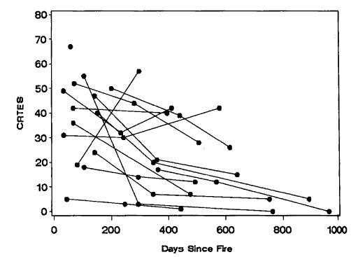
Plots of CRTES scores for 15 study participants.
In studying Figure 1, first note that not all children and adolescents were available for all three assessments. Careful scrutiny of the trajectories shows that two children or adolescents were assessed on two occasions, not three. Additionally, the single dot indicates that this child or adolescent was assessed on only one occasion early on in the study and, interestingly, had the highest CRTES score of the 15 children and adolescents in this subsample. Second, there are different patterns of responding, with some individuals recovering from initial high distress, others having exacerbations of symptoms over time, and still others having relatively “flat” trajectories, both symptomatic and asymptomatic. Third, and germane to the timing issues addressed here, initiation of assessments and intervals between assessments differ among participants.
Figure 2 (panels A, B, and C) further explores the variations in timing of assessments across participants by depicting the distributions of the number of days since the fire for each assessment occasion. Note that the number of respondents declines over assessment occasions, beginning with the full 162 cases (panel A), then dropping to 104 cases at the second assessment (panel B), and 73 cases at the third assessment (panel C). All three distributions are somewhat positively skewed and have wide dispersions. If one were to assign common times of assessment (ats) to each individual’s set of CRTES scores—either preplanned or targeted times or averages for the assessment occasions—it is conceivable that the Δatis, the differences between the individual’s targeted or average times and actual times, could affect the results. A way to reduce the Δatis is to restructure the data by reassigning individual scores from simply occasions of measurement into the time segments or time classes to which they belong. Then, one would assign a common at to each individual with CRTES scores falling within a time class, the mean or some other relevant time basis.
Figure 2.
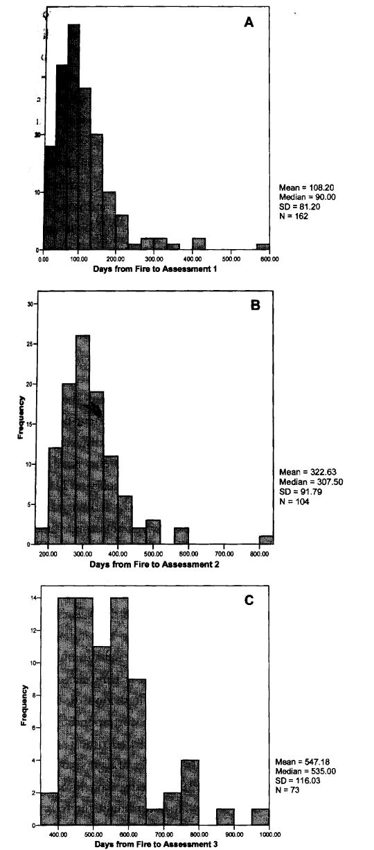
Distributions of number of days since fire for three assessment occasions.
In Table 1, we have pursued this strategy by developing alternative time structures for the Jones–Ollendick data. The topmost part of the table presents the assessment occasions-based configuration (drawn from information displayed in Figure 2). In the middle section, the structure contains four time classes: 0–180,181–360, 361–540, and >540 days. Individuals’ CRTES scores are now assigned to or associated with the time class intervals within which the assessments were conducted. The number of repeated assessments of PTSD has increased from three to four, but, importantly, scores are more faithfully linked to time since exposure. In the lower part of the table, this process is extended to 120-day time classes (1–120, 121–240, 241–360, 361–480, 481–600, and >600 days), providing six repeated assessments of PTSD. Progressing from the first to the third structure, standard deviations of the number of days within time classes have generally decreased as the number of time classes increases; the last class intervals for the 180-day and 120-day structures, which hold fewer scores, are obviously affected by extreme scores within these subsets. Hence, the reduced dispersion within time classes affords the potential for selecting a value of at, the common time of assessment assigned to each time class in SEM, that is closer to each individual’s specific time of assessment and thus yields a reduced value of Δati. Consequently, estimates of individual level and slope would be expected to be more accurate, and model-data fit would be enhanced.
Table 1.
Descriptive Statistics (Days Since Fire) for Alternative Time Structures
| Occasions-based structure | ||||||
|---|---|---|---|---|---|---|
| Occasion 1 | Occasion 2 | Occasion 3 | ||||
| n | 162 | 104 | 73 | |||
| Days M | 108.20 | 322.63 | 547.18 | |||
| Day SD | 81.20 | 91.79 | 116.03 | |||
| Structure based on 180-day time classes | ||||||
| 0–180 | 181–360 | 361–540 | >540 | |||
| n | 144 | 87 | 56 | 34 | ||
| Days M | 87.97 | 279.72 | 451.48 | 635.59 | ||
| Days SD | 44.11 | 46.24 | 48.34 | 96.10 | ||
| Structure based on 120-day time classes | ||||||
| 0–120 | 121–240 | 241–360 | 361–480 | 481–600 | >600 | |
| n | 111 | 54 | 67 | 42 | 34 | 17 |
| Days M | 68.08 | 174.57 | 298.93 | 425.07 | 545.56 | 696.06 |
| Days SD | 29.77 | 36.08 | 32.63 | 32.68 | 34.95 | 104.92 |
LATENT GROWTH CURVE ANALYSES WITH VARYING REPRESENTATIONS OF TIME
The literature on psychological trauma might suggest that the function that best describes postexposure symptom manifestation is not straight linear (e.g., Gilboa-Schectman & Foa, 2001). Indeed, King et al. (2003), with emergency room patients, and Koss and Figueredo (2004), with sexual assault victims, demonstrated a function that was linear in the logarithm of time and hence curvilinear in time, the modal trend being a sharper drop in symptom severity early on, and a tendency toward flattening out as time progresses. The CRTES means for the Jones–Ollendick data (24.02, 18.47, and 15.26 for the three assessment occasions) and an overall examination of the full complement of trajectories for these children and adolescents likewise suggested a curvilinear relationship between time and CRTES scores. Therefore, in this demonstration of latent growth curve analyses, we evaluated models in which CRTES score was regressed on the natural logarithm of time since exposure.
Four analyses were performed using the Jones–Ollendick data. Two analyses were assessment occasions-based. The first represented time (at) as the natural logarithm of the sequence of assessment events (i.e., simply the natural logarithm of 1 to represent occasion 1, natural logarithm of 2 to represent occasion 2, and natural logarithm of 3 to represent occasion 3). The second variation of occasions-based analysis indexed time (at) as the natural logarithm of the average number of days since the fire for occasions 1, 2, and 3 (using the days mean values in the upper part of Table 1). The third analysis employed the 180-day alternative time structure and indexed time (at) as the natural logarithm of the average number of days since the fire for each of the four time classes (using the days mean values in the middle section of Table 1). The fourth analysis relied on data corresponding to the 120-day time structure and represented time (at) as the natural logarithm of average number of days since the fire for each of the six time classes (using days mean values in the lower part of Table 1). Accordingly, the four analyses were designated: (a) occasions-based, natural log of 1–3; (b) occasions-based, natural log of average days; (c) 180-days-based, natural log of average days; and (d) 120-days-based, natural log of average days. For all models, time was centered on the initial assessment, level and slope were specified to covary, residual variances were constrained to be equal, and six parameters were estimated using identical data. These parameters were mean initial status or level, mean change or slope, level variance, slope variance, covariance between level and slope, and value of the residual variances.
To evaluate the models and select the best time basis, we relied primarily on the deviance, which is a function of the logarithm of the likelihood of the data, given the proposed model and the resulting parameter estimates. The greater the likelihood, the better the model-data fit, and the smaller the value of the deviance. Since the data are exactly the same for all models, all models estimate the same six parameters, and the models differ only in how time is specified, the representation of time that most likely produced the data would naturally be the one for which the deviance registers the smallest value. Hence, the deviance allows a straightforward comparison among models for the best representation of time for these particular data.
Table 2 displays the results in terms of the deviance and estimates of the six parameters for each of the four models. The values for deviance indicate that the most promising model was that based on four time classes, the model designated as 180-days-based, natural log of average days. As opposed to the two occasions-based models, this 180-days-based model directly linked CRTES scores to time classes rather than simply to assessment occasions. Also, for this 180-days-based model, the data were less sparse across time classes when compared to the data for the 120-days-based model. Recall, there are a maximum of three data points per participant. The 180-days-based model distributed these data points over four time classes, whereas the 120-days-based model distributed them over six time classes. Thus, the 180-days-based model perhaps provides more-stable parameter estimates, and therefore lower deviance values. Interestingly, for the two occasions-based models, there is little difference in the values of the deviance between occasions-based, natural log of 1–3 and occasions-based, natural log of average days. Yet, the residual variances for these two models, a function of the deviations of observed scores from predicted scores, favor the latter model: The occasions-based, natural log of average days estimate of 100.37 is lower than that of the occasions-based, natural log of 1–3 estimate of 119.49, suggesting that predicted CRTES scores are closer to the observed scores when an average-days index of time is used.
Table 2.
Four Latent Growth Curve Models With Variation in the Representation of Time
| Occasions-based natural log of 1–3
|
Occasions-based natural log of average days
|
180-days-based natural log of average days
|
120-days-based natural log of average days
|
|||||
|---|---|---|---|---|---|---|---|---|
| Estimate | SE | Estimate | SE | Estimate | SE | Estimate | SE | |
| Deviancea | 2670.83 | 2668.95 | 2630.33 | 2670.29 | ||||
| Level mean | 24.05 | 1.25 | 24.17 | 1.28 | 24.59 | 1.34 | 24.93 | 1.49 |
| Slope mean | −7.38 | 1.50 | −1.17 | 0.25 | −1.17 | 0.26 | −1.05 | 0.29 |
| Level variance | 137.51 | 34.21 | 164.98 | 34.80 | 170.45 | 36.46 | 157.23 | 40.99 |
| Slope variance | 18.47 | 52.06 | 1.99 | 1.37 | 2.02 | 1.39 | 1.74 | 1.53 |
| Level-slope covariance | −17.41 | 33.99 | −8.46 | 5.55 | −9.17 | 5.80 | −6.53 | 6.39 |
| Residual variances | 119.49 | 20.18 | 100.37 | 18.08 | 102.10 | 17.48 | 112.53 | 17.39 |
–2LL (–2 times the logarithm of the likelihood of the data given the model).
Turning to the other parameter estimates, one notes a general similarity in the estimates of initial status or level mean across the four models, and the standard errors of these estimates are likewise comparable. Because the slopes reflect the time metric, the slope indexed by the occasions-based, natural log of 1–3 is much larger than the other three slopes derived for models using natural log of average days. These three average-days-based slope means are rather consistent over time structures. Assuming normality, it is likely that the distribution of slopes for these three models would include both positive and negative individual slopes [i.e., referencing a 95% interval developed as slope mean ± (1.96)(slope variance)½], which appears to be consistent with visual inspection of trajectories for this dataset (see the subsample in Figure 1). Conversely, this result was not obtained for the occasions-based, natural log of 1–3 model.
In summary, among the four approaches to indexing time with the Jones–Ollendick data, the most enthusiasm might be expressed for the model designated as 180-days-based, natural log of average days. For this model, the deviance statistic is the smallest and the model allows for the estimation of both positive and negative individual slope statistics.
FACTORS THAT INFLUENCE TIMING OF ASSESSMENTS
As noted previously, researchers target appropriate times for assessment, primarily driven by theory. But the reality of securing initial and ongoing participation of trauma victims often results in deviations from the ideal. Participation may depend on factors that are not mandated by the design or under the control of the researcher, and any of the array of risk and resilience factors for trauma sequelae may relate to timing of assessments. Severity of exposure, for example, may play a role, in that the more disabled victims are more readily accessible and easily recruited (from hospitals or shelters), or they may suffer higher levels of distress and hence be less willing or able to make themselves available. Also, women are more likely than men to volunteer for research and thus may more readily accommodate data collection schedules, but, conversely, perhaps women have fewer resources (e.g., transportation) and more burdens (e.g., caregiving) that render them less capable of meeting appointments. If relationships between individual difference characteristics and the timing of assessments exist, they must be considered in data analysis.
One might relate putative covariates to an index of the timing of assessments. While straightforward, another approach is to place time into an event-occurrence framework (Singer & Willett, 2003). Here, the outcome is a function of the relationship between time and the probability that the individual is assessed at a given time. To illustrate, we first used the Jones-Ollendick data to calculate simple correlations between the logarithm of days since the fire to first assessment and five other variables: gender, age, minority status (member of a racial or ethnic minority group or not), CRTES score, and depression as measured by the Children’s Depression Inventory (Kovaks, 1992) at first assessment. Gender, age, CRTES score, and depression had negligible associations with the time variable (r= −.08–.05). Minority status, however, correlated r= −.20(N = 162, p < .05), with minority children’s and adolescents’ initial assessment occurring closer to the fire. To further explore this association, we estimated a proportional hazards model (Cox, 1972), based on the logarithm of the ratio of the number of individuals experiencing a certain event (first assessment) at a given time to the number of individuals still available for first assessment at that time or later. This outcome was regressed on minority status, yielding a significant χ2 (1,N= 162) = 13.48, p < .001.
Figure 3 portrays survival functions for minority and nonminority children and adolescents. The vertical axis is the probability of not experiencing the event (the event being the first assessment), and the horizontal axis is days since the fire. The figure provides a profile of the process of enrollment and initial assessment. Among those who begin study participation within the first two months (~65 days), minority children and adolescents are slightly more likely to be enrolled earlier than their nonminority counterparts. At that point, the discrepancy in probabilities widens, well into the 6-month range (~175 days); by 300 days, all minority children and adolescents have been initially assessed, but nonminority children and adolescents continue to be recruited. This strategy provides more intimate knowledge of systematic influences in the recruitment and assessment process. In fact, Jones and Ollendick (1992) made special efforts to enlist minority participants, reaching out specifically to minority community gatekeepers and organizations and minority emergency services personnel; minority recruiters and interviewers were employed, and cities with large minority populations were targeted for the study. The strategy also motivates, in this case, inclusion of minority status in analyses examining factors influencing change over time. Generally, demographic or individual difference characteristics might be treated similarly in longitudinal trauma research. Singer and Willett (2003) furnished an integration of longitudinal methods drawn from both latent growth curve and event-occurrence literatures; also see Hosmer and Lemeshow (1999) for a fuller exposition of survival analysis.
Figure 3.
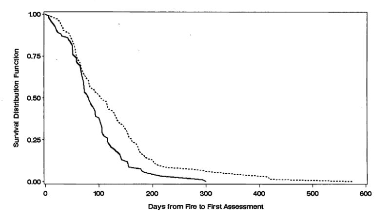
Survival functions for minority (solid line) and nonminority (broken line) children and adolescents.
SUMMARY AND CONCLUSIONS
Our goal in this article is to encourage researchers to think more seriously about the timing of assessments in longitudinal trauma research. In any longitudinal research enterprise, especially one in which there is an expected developmental component, that is, the prospect of intensification or deterioration in some noteworthy outcome, an accurate portrayal of time and its consideration within data analysis is quite important. In trauma research, there is typically a discrete starting point, the time of exposure to a traumatic event, and the timing of our observations are thus linked to a developmental sequence. Yet, we should recognize that timing of assessments in longitudinal trauma research can be inconsistent across participants and quite disparate from what was formally proposed and intended.
We advocate for descriptive and graphical examination of the trends and patterns for the outcome variable(s) at the level of individual study participants (as demonstrated here in Figure 1 with the Jones–Ollendick data). We especially recommend scrutiny of the characteristics of the distributions of the timing of assessments (as portrayed in Figure 2). These very simple practices can reveal both variations in the timing of assessments and possibly inform more veridical functions that can best describe the process of change in the outcome(s) over the course of the study.
The flexibility of the SEM-based approach vis-à-vis structural model specification and error structures makes it particularly attractive for longitudinal investigations, but it requires a specification of a common time basis for all cases. It is worthwhile to explore variations in time structures (as we did in Table 1) to capture a reliable representation of change that is amenable to the SEM-based repertoire. We also suggested a strategy (see Table 2) using the deviance statistic and values of the parameter estimates to assist in determining the best time basis for SEM analysis. This strategy, of course, requires specification of a plausible change function underlying the data, derived from theory, prior research, and direct observation of the trajectories apparent in the data set under scrutiny (again, see Figure 1).
Finally, researchers might consider existing tools to better understand how data collection unfolds over time. Simple correlations and event-occurrence methods can assist in understanding relationships between research-relevant individual difference characteristics (or other features of the study) and the timing of assessments. Plots such as Figure 3 highlight the process of study entry and reveal how such variables could confound time-outcome relationships. Here, we demonstrated the analysis of a single event (first assessment), but techniques are available (Singer & Willett, 1995) to simultaneously examine multiple events, where some factor might differentially affect the timing of subsequent assessments (e.g., time from first to second assessment, from second to third assessment).
Acknowledgments
This study was supported by a National Institute of Mental Health grant (“New Longitudinal Methods for Trauma Research,”5RO1MH68626-2, Daniel W. King, Principal Investigator). Additional support was provided by the Massachusetts Veterans Epidemiology Research and Information Center (MAVERIC). We would like to thank Susan Doron-LaMarca for assistance with data management and analysis.
Footnotes
In the remainder of this article, comments concerning time are in the context of time since exposure to a traumatic event. They can, however, be extrapolated to time since any event, including the initiation or termination of an intervention.
As will he noted later, a straight-line trajectory of posttrauma change is likely not the best model.
The model can be parameterized such that Leveli, represents an individual’s score on any assessment occasion (see Biesanz, Deeb-Sossa, Papadakis, Bollen, & Curran, 2004).
We have selected this term as the generic expression, since it is used in both the structural equation modeling context (e.g., Muthén, 2000) and the multilevel regression context (e.g., Raudenbush & Bryk, 2002).
References
- Biesanz JC, Deeb-Sossa N, Papadakis AA, Bollen KA, Curran P. The role of coding time in estimating and interpreting growth curve models. Psychological Methods. 2004;9:30–52. doi: 10.1037/1082-989X.9.1.30. [DOI] [PubMed] [Google Scholar]
- Cox DR. Regression models and life tables. Journal of the Royal Statistical Society. 1972;34:187–202. [Google Scholar]
- Cronbach LJ, Furby L. How should we measure change—Or should we? Psychological Bulletin. 1970;74:68–80. [Google Scholar]
- Denny N, Robinowitz R, Penk W. Conducting applied research on Vietnam combat-related post-traumatic stress disorder. Journal of Clinical Psychology. 1987;43:56–66. doi: 10.1002/1097-4679(198701)43:1<56::aid-jclp2270430108>3.0.co;2-d. [DOI] [PubMed] [Google Scholar]
- Erickson DJ, Wolfe J, King DW, King LA, Sharkansky EJ. Posttraumatic stress disorder and depression symptomatology in a sample of Gulf War veterans: A prospective analysis. Journal of Consulting and Clinical Psychology. 2001;69:41–49. doi: 10.1037//0022-006x.69.1.41. [DOI] [PubMed] [Google Scholar]
- Gilboa-Schectman E, Foa EB. Patterns of recovery from trauma: The use of intraindividual analysis. Journal of Abnormal Psychology. 2001;110:392–400. doi: 10.1037//0021-843x.110.3.392. [DOI] [PubMed] [Google Scholar]
- Gollob HR, Reichardt CS. Taking account of time lags in causal models. Child Development. 1987;58:80–92. [PubMed] [Google Scholar]
- Green BL, Lindy JD, Grace MC. Post-traumatic stress disorder: Toward DSM-IV. Journal of Nervous Mental Disorders. 1985;173:406–411. doi: 10.1097/00005053-198507000-00004. [DOI] [PubMed] [Google Scholar]
- Hosmer DW, Lemeshow S. Applied survival analysis: Regression modeling of time to event data. New York: Wiley; 1999. [Google Scholar]
- Humphreys LG. Linear dependence of gain scores on their components imposes constraints on their use and interpretation: Comment on “Are simple gain scores obsolete? Applied Psychological Measurement. 1996;20:293–294. [Google Scholar]
- Jones RT. Child’s Reaction to Traumatic Events Scale (CRTES): Assessing traumatic experiences in children. In: Wilson JP, Keane T, editors. Assessing psychological trauma & PTSD. New York: Guilford Press; 1996. pp. 291–298. [Google Scholar]
- Jones RT, Ollendick TH. Residential fires. In: La Greca AM, Silverman WK, Vernberg EM, Roberts MC, editors. Helping children cope with disasters and terrorism. Washington DC: USical Association; 2002. pp. 175–199. [Google Scholar]
- Keane TM, Wolfe J, Taylor K. Posttraumatic stress disorder: Evidence for diagnostic validity and methods of psychological assessment. Journal of Clinical Psychology. 1987;43:32–43. doi: 10.1002/1097-4679(198701)43:1<32::aid-jclp2270430106>3.0.co;2-x. [DOI] [PubMed] [Google Scholar]
- King DW, King LA. Validity issues in research on Vietnam veteran adjustment. Psychological Bulletin. 1991;109:107–124. doi: 10.1037/0033-2909.109.1.107. [DOI] [PubMed] [Google Scholar]
- King DW, King LA, Erickson DJ, Huang MT, Sharkansky EJ, Wolfe J. Posttraumatic stress disorder and retrospectively reported stressor exposure: A longitudinal prediction model. Journal of Abnormal Psychology. 2000;109:624–633. doi: 10.1037//0021-843x.109.4.624. [DOI] [PubMed] [Google Scholar]
- King LA, King DW, Salgado DM, Shalev AY. Contemporary longitudinal methods for the study of trauma and stress. CNS Spectrums. 2003;8:686–692. doi: 10.1017/s1092852900008877. [DOI] [PubMed] [Google Scholar]
- King DW, Tart CT, King LA, Hammond C, Stone ER. Directionality of the association between social support and posttraumatic stress disorder: A longitudinal investigation. Journal of Applied Social Psychology in press. [Google Scholar]
- King DW, Vogt DS, King LA. Risk and resilience factors in the etiology of chronic PTSD. In: Litz BT, editor. Early interventions for trauma and traumatic loss in children and adults: Evidence-based directions. New York: Guilford Press; 2004. pp. 34–64. [Google Scholar]
- Koss MP, Figueredo AJ. Change in cognitive mediators of rape’s impact on psychosocial health across 2 years of recovery. Journal of Consulting & Clinical Psychology. 2004;72:1063–1072. doi: 10.1037/0022-006X.72.6.1063. [DOI] [PubMed] [Google Scholar]
- Kovacs M. Manual. Toronto, Ontario, Canada: Multi-Health Systems, Inc; 1992. The Children’s Depression Inventory (CDI) [Google Scholar]
- McArdle JJ, Woodcock RW. Expanding test-retest designs to include developmental time-lag components. Psychological Methods. 1997;2:403–435. [Google Scholar]
- Muthén B. Growth modeling with binary responses. In: Von Eye A, Clogg C, editors. Categorical variables in developmental research: Methods of analysis. San Diego, CA: Academic Press; 1996. pp. 37–54. [Google Scholar]
- Muthén B. Methodological issues in random coefficient growth modeling using a latent variable framework: Applications to the development of heavy drinking in ages 18–37. In: Rose JS, Chassin L, Presson CC, Sherman SJ, editors. Multivariate applications in substance use research: New methods for new questions. Mahwah, NJ: USum Associates; 2000. pp. 113–140. [Google Scholar]
- Nesselroade JR, Cable DG. “Sometimes, it’s okay to factor difference scores”—The separation of state and trait anxiety. Multivariate Behavioral Research. 1974;9:273–281. doi: 10.1207/s15327906mbr0903_3. [DOI] [PubMed] [Google Scholar]
- Orcutt HK, Erickson DJ, Wolfe J. The course of PTSD symptoms among Gulf War Veterans: A growth mixture modeling approach. Journal of Traumatic Stress. 2004;17:195–202. doi: 10.1023/B:JOTS.0000029262.42865.c2. [DOI] [PubMed] [Google Scholar]
- Raudenbush SW, Bryk AS. Hierarchical linear models: Application and data analysis methods. Thousand Oaks, CA: Sage; 2002. [Google Scholar]
- Resnick HS, Acierno R, Waldrop A, King LA, King SW, Danielson C . Evaluation of a randomized early intervention to prevent post-rape psychopathology. 2006. Manuscript submitted for publication. [DOI] [PMC free article] [PubMed] [Google Scholar]
- Schell TL, Marshall GN, Jaycox LH. All symptoms are not created equal: The prominent role of hyperarousal in the natural course of posttraumatic psychological distress. Journal of Abnormal Psychology. 2004;113:189–197. doi: 10.1037/0021-843X.113.2.189. [DOI] [PubMed] [Google Scholar]
- Sharma KK, Gupta JK. Optimum reliability of gain scores. Journal of Experimental Education. 1986;54:105–108. [Google Scholar]
- Singer JD, Willett JB. It’s déjà vu all over again: Using multiple-spell discrete-time survival analysis. Journal of Educational and Behavioral Statistics. 1995;20:41–67. [Google Scholar]
- Singer JD, Willett JB. Applied longitudinal data analysis: Modeling change and event occurrence. London: Oxford University Press; 2003. [Google Scholar]
- Williams RH, Zimmerman DW. Are simple gain scores obsolete? Applied Psychological Measurement. 1996;20:59–69. [Google Scholar]
- Willett JB, Sayer AG. Using covariance structure analysis to detect correlates and predictors of individual change over time. Psychological Bulletin. 1994;116:363–381. [Google Scholar]