

Abstract
We contrasted coherence estimates obtained with EEG, Laplacian, and MEG measures of synaptic activity using simulations with head models and simultaneous recordings of EEG and MEG. EEG coherence is often used to assess functional connectivity in human cortex. However, moderate to large EEG coherence can also arise simply by the volume conduction of current through the tissues of the head. We estimated this effect using simulated brain sources and a model of head tissues (CSF, skull, and scalp) derived from MRI. We found that volume conduction can elevate EEG coherence at all frequencies for moderately separated (< 10 cm) electrodes; a smaller elevation is observed with widely separated (> 20 cm) electrodes. This volume conduction effect was readily observed in experimental EEG at high frequencies (40-50 Hz). Cortical sources generating spontaneous EEG in this band are apparently uncorrelated. In contrast, while lower frequency EEG coherence appears to result from a mixture of volume conduction effects and genuine source coherence. Surface Laplacian EEG methods minimize the effect of volume conduction on coherence estimates by emphasizing sources at smaller spatial scales than unprocessed potentials (EEG). MEG coherence estimates are inflated at all frequencies by the field spread across the large distance between sources and sensors. This effect is most apparent at sensors separated by less than 15 cm in tangential directions along a surface passing through the sensors. In comparison to long-range (> 20 cm) volume conduction effects in EEG, widely spaced MEG sensors show smaller field spread effects, which is a potentially significant advantage. However, MEG coherence estimates reflect fewer sources at a smaller scale than EEG coherence and may only partially overlap EEG coherence. EEG, Laplacian, and MEG coherence emphasize different spatial scales and orientations of sources.
Introduction
The central goal of EEG studies is to relate various measures of neural dynamics to functional brain state, determined by behavior, cognition, or neuropathology. One of the most promising measures of such dynamics is coherence, a correlation coefficient (squared) that estimates the consistency of relative amplitude and phase between any pair of signals in each frequency band (Bendat and Piersol, 2000). Any pair of EEG signals may be coherent in some frequency bands and incoherent in others; the dependence of detailed extracranial coherence patterns on frequency and brain state is now well established (Nunez, et al. 1997; 1999; 2001; Silberstein et al., 2003, 2004; Srinivasan 1999; Srinivasan et al., 1999; Nunez and Srinivasan, 2006a). EEG coherence provides one important estimate of functional interactions between neural systems operating in each frequency band. EEG coherence may yield information about network formation and functional integration across brain regions.
The coherence measure is generally distinct from synchrony (Singer, 1999), which in the neuroscience literature normally refers to signals oscillating at the same frequency with identical phases. This type of synchronization in a local region of cortex is a critical factor in determining EEG amplitude in the same (centimeter scale) region. That is, each EEG signal is generated by a superposition of many brain current sources (Nunez and Srinivasan, 2006a); the contribution of each source depends on source and electrode locations and the spread of current through the head volume conductor. Each EEG electrode signal reflects an average over all sources in a large region of the cortex (on the order of 100 cm2), and synchronous sources within this region produce much larger signals at each electrode than asynchronous sources. Thus, EEG amplitude in each frequency band can be related to the synchrony of the underlying current sources (Nunez and Srinivasan, 2006a). Consistent with this argument, reduction in amplitude is often labeled desynchronization (Pfurtscheller and Lopes da Silva, 1999). Of course, reduction in amplitude may, in theory, occur as a result from either reduction in (mesosocopic) source magnitude or reduction in the surface area this synchronized (Nunez and Srinivasan, 2006a).
In contrast to amplitude measures, coherence is a measure of synchronization between two signals based mainly on phase consistency; that is, two signals may have different phases (as in the case of voltages in a simple linear electric circuit), but high coherence occurs when this phase difference tends to remain constant. In each frequency band, coherence measures whether two signals can be related by a linear time invariant transformation, in other words a constant amplitude ratio and phase shift (delay). In practice, EEG coherence depends mostly on the consistency of phase differences between channels (Nunez, 1995; Nunez and Srinivasan, 2006a). High coherence between two brain areas is an indicator that the relationship between the signals generated in such areas may be well approximated by a linear transformation; however, this does not necessarily imply that the underlying neocortical dynamics is linear.
While there has been a great deal of interest in using EEG coherence to measure functional connectivity in the brain, one serious limitation of extracranial EEG coherence measures is contamination by volume conduction through the tissues separating sources and electrodes. We have investigated this effect theoretically using 4-sphere models of volume conduction consisting of an innermost sphere representing the brain surrounded by three concentric spherical shells representing cerebrospinal fluid (CSF), skull, and scalp (Nunez, 1981; Srinivasan et al., 1998). When all cortical sources are uncorrelated, i.e., incoherent in every frequency band, this model predicts substantial EEG scalp coherence at electrode separations less than approximately 10 to 12 cm (Nunez et al., 1997, 1999; Srinivasan et al., 1998). A small volume conduction effect is also predicted for very large electrode separations (> 20 cm). The volume conduction effect is independent of frequency and depends only on the electrode locations and electrical properties of the head. In the 4-sphere model, electrodes separated by less than about 10 to 12 cm are apparently recording from partly overlapping source distributions due to volume conduction. As the separation distance between electrodes decreases, the overlap in source distributions and coherence due to volume conduction both increase. This picture is qualitatively consistent with a variety of experimental EEG data (Srinivasan et al., 1998; Srinivasan, 1999; Nunez 1981, 1995; Nunez and Srinivasan, 2006a). Two nearby EEG electrodes will appear coherent across all frequency bands because they record potentials generated by some of the same sources. In an earlier paper (Nunez et al., 1997), we defined “reduced coherence” as the difference between the measured EEG coherence and the “random coherence”, defined as the scalp EEG coherence due only to volume conduction expected when cortical sources are uncorrelated. However, volume conduction distortions of coherence are not simply additive but reflect spatial filtering of source activity (Srinivasan et al., 1998). Reduced coherence is only a crude idea of the general magnitude of source coherence based on a rough estimate of volume conduction effects.
We can partly overcome this problem of EEG coherence due to volume conduction by reducing the spatial scale of scalp potentials with high resolution EEG methods like the surface Laplacian (Law et al., 1993; Nunez et al., 1991, 1993, 1997, 1999; Perrin et al., 1987, 1989; Srinivasan et al., 1996; Nunez and Srinivasan, 2006a). The surface Laplacian is the second spatial derivative of the scalp potential in two surface coordinates tangent to the local scalp. In simulations with 4-sphere models, the spatial area averaged by each electrode is reduced from perhaps 100 cm2 for (average reference) scalp potentials to perhaps 10 cm2 for spline Laplacians estimated from dense electrode arrays (e.g., 131 electrodes, 2.2 cm center-to-center average spacing, Nunez et al., 2001). Our simulations with 4-sphere models indicate that all volume conduction effects are removed from Laplacian coherence estimates at distances greater than about 3 cm (Srinivasan et al., 1998; Nunez et al., 1997, 1999; Nunez and Srinivasan, 2006a). The surface Laplacian isolates the source activity under each electrode that is distinct from the surrounding tissue under adjacent electrodes such that measured Laplacian coherence can be directly related to coherence between these sources. However, Laplacians may also remove genuine source coherence associated with widely distributed source regions (very low spatial frequencies) along with volume conduction contributions; that is, the Laplacian spatial filter cannot distinguish between source and volume conduction effects. In other words, Laplacian coherence provides estimates of the phase consistency of sources at smaller spatial scales in comparison to (average reference) EEG coherence (Nunez and Srinivasan, 2006a).
MEG (magnetoencephalography) is a relatively new technology that potentially provides useful insights into brain sources (Hamaleinen et al., 1993), especially when used as an adjunct to EEG measurements (Nunez and Srinivasan, 2006a). One common but erroneous idea is that MEG spatial resolution is inherently superior to EEG spatial resolution, and that MEG should simply replace EEG in order to extract more accurate information about brain source dynamics. Because of the large distance separating the magnetometer coils from the sources (typically 3-4 cm above the scalp), MEG also yields relatively large extracranial coherence even when the underlying brain sources are uncorrelated due to the effects of field spread to the sensors (Srinivasan et al., 1999; Winter et al; 2006). The main distinction between MEG and EEG measures is that they are selectively sensitive to different source orientations; this can be either an advantage or disadvantage for MEG depending on application. One clear advantage of MEG over EEG is that much less detailed knowledge of the volume conductive and geometrical properties of the head is required to model the signals. Since normal tissue is nonmagnetic, (magnetic) permeability (μ) is constant across head tissues and free space; to first approximation, the magnetic field depends only on the locations and orientations of sources and sensors (Hamalainen et al., 1993).
Our earlier studies (Nunez et al., 1997; Srinivasan et al., 1998) using the 4-sphere head model made use of exclusively radial dipoles sources (representing gyral surfaces) forming a spherical layer. EEG is more sensitive to radial sources than tangential sources at any depth in the 4-sphere model (Nunez and Srinivasan, 2006a). Coherence due to volume conduction may be expressed analytically using the 4-sphere model when the source distribution forms a spherical layer (Srinivasan et al., 1998). This analytic expression generally agrees with observed volume conduction effects in EEG recordings. Although radial dipoles appear adequate for most EEG effects, tangential sources are essential for modeling field spread effects on MEG coherence and are likely also to make contributions to EEG volume conduction effects. The local tangential sources depend on the geometry of cortical folds; thus attendant simulations require dipoles at realistic cortical locations.
The goal of this paper is to model the relationship between brain source dynamics and extracranial MEG and EEG dynamics in order to interpret the physiological bases of measured coherence. We use MRI to model the cortical surface in order to realistically position and orient dipole sources in a 3-ellipsoid model of the head (brain, skull, and scalp). In contrast, our previous models of volume conduction effects on EEG coherence used concentric spheres, and exclusively superficial radial dipoles. With the new ellipsoidal model and realistic source geometry, we quantify the spatial resolutions of conventional EEG, Laplacian, and MEG and estimate the effects of volume conduction (EEG, Laplacian) and separation of sources from sensors (EEG, Laplacian, MEG) on coherence measures. We compare our model results to EEG, Laplacian, and MEG measures of coherence obtained from simultaneous 148 channel MEG and 127 channel EEG recordings. Our results confirm that both the location and the spatial scale of brain networks determine the patterns of EEG, Laplacian, and MEG coherence.
Methods
Experimental methods
Data were recorded in six subjects at the Scripps Research Foundation in La Jolla, CA: 127 EEG channels (Advanced Neuro Technology, Enschede, The Netherlands) and 148 MEG channels (4D Neuroimaging, San Diego, USA). The EEG amplifier was powered with a battery and placed inside the shielded room, and fiber-optic cables were used to transmit the EEG signals to the acquisition computer outside the room. The EEG and MEG signals were analog filtered at 100 and 108 Hz and sampled at 940 Hz and 1018 Hz, respectively. Because the EEG and MEG signals were sampled by independent amplifiers and A/D cards, triggers were used to denote transitions between experimental states. This ensured that the two data sets had sample-to-sample correspondence, verified by the alignments of random trigger signals (+5 V) that were sampled by both the EEG and MEG systems during each recording.
Procedure
The first experimental procedure consisted of a four minute period with subjects resting with eyes-closed followed by four minutes with resting, eyes-opened. In addition, four one minute periods of eyes closed resting were alternated with a (eyes closed) mental arithmetic task chosen to manipulate coherence patterns (Nunez, 1995; Nunez et al., 2001). Each subject was given a random two digit number X and asked to mentally sum the series X+1, (X+1)+2, (X+1+2)+3 … to sums of several hundred. Six subjects participated in the experiment; a high-resolution (1mm × 1mm × 1mm) MRI scan was also acquired on a separate day from three subjects.
Surface Laplacian
The surface Laplacian was estimated from the New Orleans spline Laplacian algorithm (Law et al., 1993; Nunez et al., 1993; Srinivasan et al., 1996; Nunez and Srinivasan, 2006a). The spline Laplacian is based on three-dimensional interpolation of discrete samples of scalp potential with a best fit sphere to the scalp surface used to estimate the two surface derivatives at each electrode location; its accuracy has been verified in thousands of simulations. Because Laplacian estimates are generally inaccurate at the locations of edge electrodes (Srinivasan et al., 1998; Nunez et al., 2001), all coherence estimates involving the 18 edge electrodes in simulations and genuine data were excluded from our results.
Coherence analysis
The data were resampled to 128 Hz using the Matlab (Natick, MA) resample function. Alignment of trigger signals was used to verify alignment of EEG and MEG after resampling. The data were divided into 2-second epochs and detrended. Estimated equipment and room noise were removed from the raw MEG data by digital filtering using reference coils positioned in the dewar above the array of MEG coils (Srinivasan et al., 1999). Amplitude thresholds of 70 μV for EEG and 5 pT for MEG were used to eliminate epochs containing high-amplitude artifact; typically, 80% of epochs were retained in each experiment with these thresholds. The EEG data were referenced to the average potential of all channels (the standard average reference potential that approximates potential at infinity, see Nunez and Srinivasan, 2006a).
The Matlab FFT algorithm was applied to each 2-second epoch of data yielding Fourier coefficients with frequency resolution Δf = 0.5 Hz at each of the m = 1, M channels for epochs k = 1, K, with K = 120 epochs in each brain state. The cross spectrum estimate based on the complex valued coefficients Fuk (fn), Fuk (fn) for channel pair (u,v) is
| (1) |
For single channels (u = v) the cross-spectrum reduces to the usual power spectrum Pu(fn) = Guu(fn). Coherence at each frequency is the normalized cross spectrum, estimated by (Bendat and Piersol, 2000)
| (2) |
Coherence was calculated between all pairs of data channels within each of the measurement categories, EEG, Laplacian and MEG.
MRI based source models
In order to simulate EEG and MEG coherence effects due to the separation of sensors from sources, dipoles at realistic cortical locations are required. Sources in the 3-ellipsoid model follow the cortical surfaces obtained from MRIs of individual subjects. While mainly motivated by the need to study MEG coherence, we note that omission of tangential dipoles could possibly also have important influences on our estimates of the EEG or Laplacian coherence due to volume conduction. The source models used in this study were based on MRIs obtained on three subjects. Grid surfaces were created to represent the brain by a combination of automatic segmentation with a threshold and manual correction of the segmented volume on a slice-by-slice basis (Brain Voyager QX 1.6, Brain Innovation B.V., Maastricht, The Netherlands). Sources were simulated at each point of the grid representing the brain boundary as the current dipole moment per unit volume P(r,t) oriented perpendicular to the local cortical surface (for discussion of this mesoscopic source function in terms of synaptic microsources, see Nunez and Srinivasan, 2006a). An example grid is shown in Fig 1.
Figure 1.

(a) Electrode locations on the best fit ellipsoid to the scalp surface are shown as grey circles. (b) MEG coils approximately 4 cm above the scalp are shown.
3-ellipsoid volume conduction model
The upper surfaces of human heads may be fit accurately to general ellipsoids defined by their dimensions along three orthogonal axes (Law and Nunez, 1991). For purposes of this study, we have constructed new head models (for three subjects) based on three confocal ellipsoidal surfaces (3-ellipsoid models) for the following reasons: (1) The new models have a more realistic geometry (in comparison to spherical models) that may influence coherence especially at the large anterior-posterior electrode separations. However, we have not used realistic head geometry (skull and scalp) in the model partly because such models make the incorrect assumption that resistance is proportional to thickness of the skull layer. As discussed in Nunez and Srinivasan (2006a), in vivo measurement of hydrated skull plugs and in vivo studies of skull flaps in surgery patients provide no clear evidence that thicker skull has greater resistance. Rather, the thicker middle (spongy) skull layer appears to be a better conductor due its ability to hold fluid. The adoption of three confocal ellipsoids allows us to focus on the issue of non-spherical head shape and make use of realistic source geometry, without introducing factors related to tissue conductivity that are not well-known.
The CSF/skull boundary was segmented to fit a general ellipsoid by means of a principal component analysis. Two confocal ellipsoidal surfaces of constant thicknesses were then added to represent outer skull and scalp surfaces. Each of the outer ellipsoids was centered and oriented on the innermost ellipsoid (CSF/skull boundary) as shown by the scalp surface with electrode positions in Fig 1a. The thicknesses of layers were almost identical to those used in our 4-sphere model (Srinivasan et al., 1998), except for absence of the CSF layer. In general, the CSF layer is thin (< 1 to 2 mm) so that its effect on volume conduction is generally small in 4-sphere models; in any case, the effect of CSF in the 4-sphere model may be approximated in the 3-sphere model by increasing the effective skull conductivity (Nunez and Srinivasan, 2006a). The CSF/skull boundary was also fit to a sphere, and a 3-sphere model was similarly constructed. For both ellipsoidal and spherical models, the best-fit electrode positions were calculated.
The outer surface potentials for dipole sources were obtained for the 3-sphere and 3-ellipsoid models using a boundary element model (ASA 3, EEimagine, Germany). The numerical solution for outer surface potential due to a single radial dipole in the 3-sphere boundary element model was found to match the corresponding analytic solution as expected. The outer spherical surface was also used to provide a spherical surface for the New Orleans Laplacian algorithm.
Numerical solutions for outer surface potentials due to unit dipoles at each location over the folded, MRI generated model of the cortical surface were calculated with the 3-ellipsoid model. For each subject there were approximately 100,000 dipole sources per hemisphere, approximating the continuous source function P(r,t). The surface Laplacian was calculated from the potential distribution for each dipole source. This yielded two matrices for the EEG (GE) and Laplacian (GL) where each row corresponded to one dipole source and each column corresponded to the EEG electrode positions. These matrices are the numerical versions of the corresponding Green's function, a concept widely used in mathematical physics and engineering (Srinivasan et al., 1998; Nunez and Srinivasan, 2006a).
Magnetic field model
The local surface normal of the magnetic field Hn (r,t) on a ellipsoidal surface (passing through the MEG sensors) 4 cm above the scalp ellipsoid, as shown in Fig 1b was calculated from the Biot-Savart law (Nunez, 1986; Hamaleinen et al., 1993; Nunez and Srinivasan, 2006a)
| (3) |
Here the sum is over all I cortical dipoles P(ri,t)ΔV with cortical locations ri, where ΔV is the discrete volume element of cortical tissue, an (r) is a unit vector normal to the local sensor surface, and r is location on the sensor ellipsoid.
Numerical solutions for the radial magnetic field due to unit dipoles at each location over the folded, MRI generated model of the cortical surface were calculated. For each subject there were approximately 100,000 dipole sources per hemisphere. This yielded a matrix (GM) where each row corresponded to one dipole source and each column corresponded to the MEG sensor positions.
Sensitivity distribution and half sensitivity area
The sensitivity of each EEG or Laplacian electrode and MEG sensor to dipole sources on the cortical surface was expressed in terms of a sensitivity distribution. The properties of the electric and magnetic Green's functions determine the sensitivity of EEG electrodes and MEG coils as demonstrated by Malmivuo and Plonsey (1995) using lead field analysis in spherical volume conduction models. By introducing more realistically shaped volume conduction models such as ellipsoids, the sensitivity estimates are further refined by restricting the simulated sources P(r,t) to be normal to the local cortical surface derived from MRI.
For each electrode or sensor position the sensitivity distribution describes the relative contribution of each possible source to the electrode or sensor and can be obtained by normalizing each column of the Green's function matrix (GE, GL, or GM) to its maximum magnitude on the brain surface. The sensitivity function provides a simple way to visualize the locations of brain sources that make the largest contributions to EEG, Laplacian, or MEG signals. The half-sensitivity area (HSA) is the surface area (on the brain surface) which contains all the sources which contribute at least half of the strongest signal. The half-sensitivity area is similar to the half-sensitivity volume defined by Malmivuo and Plonsey (1995) and provides a simple metric of the spatial resolutions of EEG, Laplacian and MEG measures.
Spatial white-noise simulation
Spatial white noise source distributions P(r,t) over the entire brain were defined as a delta correlated random process; in other words at any frequency the cross-spectrum between all pairs of sources forms an identity matrix, KPP = I. The cross spectrum of the EEG can be calculated from the source cross-spectrum and Green's function matrix as . The cross spectrum of the Laplacian and the MEG were similarly calculated using the appropriate Green's function matrix. Cross spectra were normalized to obtain the coherence using Eq (2). In this idealized simulation (with essentially an infinite number of epochs) any nonzero coherence observed between EEG or MEG channels reflects only the effects of volume conduction or field spread. In simulations with finite number of epochs used to estimate coherence, small non-zero coherence is also observed due to statistical fluctuations.
Results
Sensitivity distributions of EEG, Laplacian, and MEG
Figure 2 shows the sensitivity distributions for a fixed EEG electrode location (yellow circle at right) and MEG coil position (green line) shown in the figure inset. We have normalized the Green's function to its maximum magnitude on the brain surface in order to define the sensitivity function that describes the contribution of each source to the electrode or sensor. Fig 2a shows that the EEG electrode is most sensitive to sources in the gyral crown closest to the electrode. Although the sensitivity function tends to fall off with distance from the electrode, gyral crowns widely distributed throughout the cortical hemisphere contribute roughly half the potential of the sources directly beneath the electrode. Sources along sulcal walls, even when close to the electrode, contribute much less to scalp potential than sources in the gyral crowns. Figure 2b shows the Laplacian sensitivity distribution for the same electrode position. The highest sensitivity regions of the Laplacian and EEG are the identical gyral crown beneath the electrode as expected. The Laplacian is much less sensitive to distant gyral crowns, thereby providing a far more “local” measure of source activity. Figure 2c shows the sensitivity distribution of an MEG coil whose location 4 cm above the EEG electrodes is shown in the inset head. Each MEG coil is sensitive to a large region of the cortex, consistent with the very large half sensitivity volumes reported for a single coil magnetometer (Malmivuo and Plonsey, 1995). The sensitivity function generally exhibits local maxima on sulcal walls. Opposing sulcal walls have opposite sensitivities because of the change in orientation of the sources; thus adjacent surfaces with sensitivities of opposite sign are expected to make only small or perhaps negligible contributions to the magnetic sensor.
Figure 2.

The EEG (a), Laplacian (b), and MEG (c) sensitivity distributions for a fixed electrode location (yellow circle at right inset figure) and magnetic coil position (green line at right inset figure) are shown. The cortical surface was constructed from the MRI of one subject. Simulated “dipole sources” P(r,t) (dipole moment per unit volume, 100,000 in one hemisphere) were assumed normal to the local cortical surface. Scalp surface potentials, scalp Laplacians, and surface normal magnetic fields due to each dipole were calculated at the electrode and coil locations shown in the inset using Green's functions (one for each measure) based on the confocal 3-ellipsoid head model. The three Green's functions were normalized with respect to their maximum values so that the relative sensitivity of the three measured could be compared. (a) The EEG electrode is most sensitive to gyral sources under the electrode, but this electrode is also sensitive to large source regions occupying relatively remote gyral crowns and much less sensitive to sources in cortical folds. (b) The Laplacian is most sensitive to gyral sources under the electrode; sensitivity falls off rapidly at moderate and large distances. (c) The MEG is most sensitive to sources in cortical folds that tend to be tangent to MEG coils. Maximum MEG sensitivity occurs in folds that are roughly 4 cm from the coil in directions tangent to the surface. Regions in blue provide contributions to MEG of opposite sign to those of yellow/orange, reflecting dipoles on opposite sides of folds that tend to produce canceling magnetic fields at the coil.
We follow the notion of a half-sensitivity volume (Malmivuo and Plonsey, 1995) in order to define a half-sensitivity area as the surface area of the cortex that contains sources that could contribute at least half the signal contributed by the strongest source location for each electrode or MEG sensor position. Across 128 electrode locations in the three subject's head models, the EEG half-sensitivity areas ranged from 8 to 35 cm2 (median = 13 cm2); across 148 sensor positions, MEG half-sensitivity area ranged from 5 to 26 cm2 (median = 11 cm2). In contrast to the widespread sensitivity areas of conventional EEG or MEG, the sensitivity area of high-resolution EEG obtained with the surface Laplacian is limited to very local sources within a small distance to the electrode. In our study, Laplacian half-sensitivity areas ranged from 0.8 to 5.1 cm2 (median = 1.5 cm2).
Figure 3a shows the half-sensitivity distribution for the potential due to two electrodes spaced by about 5 cm as shown in the figure inset. The regions of cortex associated with the half-sensitivity area of each electrode are indicated by the two colors; they are shown to overlap substantially. The dramatic improvement in spatial resolution afforded by high-resolution EEG is demonstrated by comparing these results with the corresponding surface Laplacian sensitivity plot in Figure 3b. The surface Laplacians at these two electrodes are shown to be sensitive to distinct local gyral crowns. The highest sensitivity for each electrode is at the same location in the cortex as for the potential in Fig. 3a, but the surface Laplacian is much less sensitive to more distant gyral surfaces. The implication is that if a source region is localized within a small dipole layer in a specific gyral surface as indicated in the figure, the surface Laplacian will isolate the signal corresponding to that source in a single electrode. In contrast, the same source will contribute substantially to potentials recorded at both electrodes.
Figure 3.
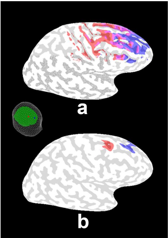
The half-sensitivity areas for the potential (a) and Laplacian (b) due to two electrodes spaced by about 5 cm (shown in the figure inset at left) are plotted using the 3-ellipsoid head model. Half-sensitivity areas are defined as the surface areas of the cortex containing sources that could contribute at least half the “maximum signal” (i.e., contributed by the strongest source location for each electrode or MEG sensor position). The regions of cortex associated with the half-sensitivity area of each electrode are indicated by the two colors. The areas associated with the scalp potential measure are shown to overlap substantially, whereas the scalp Laplacians at these two electrodes are shown to be sensitive mainly to distinct local gyral crowns reflecting the Laplacian's much improved spatial resolution.
Spatial white-noise simulations of EEG, Laplacian, and MEG coherence
Figure 4 shows simulated coherence as a function of tangential electrode (or MEG coil) separation for EEG, Laplacian, and MEG for uncorrelated cortical sources (spatial white noise at arbitrary temporal frequency) as obtained from our 3-ellipsoid head model in one subject. The simulated cortical dipoles are distributed over the entire folded cortical surface with locations in gyri and cortical folds assumed normal to the local cortical surface, obtained from the subject's MRI.
Figure 4.

Simulated coherence is shown as a function of tangential electrode (or MEG coil) separation for EEG, Laplacian, and MEG for uncorrelated cortical sources, that is, spatial white noise at arbitrary temporal frequency. Sensor separation is defined on the simulated scalp surface (ellipsoidal). These coherence fall-offs with sensor separation were calculated using our 3-ellipsoid head model. Simulated cortical dipoles P(r,t) are distributed over the entire folded cortical surface with locations in gyri and cortical folds. P(r,t) is assumed everywhere normal to the local cortical surface, as obtained from one subject's MRI. The grey lines plot the average coherence at each sensor separation.
At small to moderate electrode separations (< 10 to 12 cm) EEG appears to be somewhat coherent even when the underlying sources are uncorrelated as shown in Fig 4a. This effect is independent of temporal frequency and only reflects the overlap in sensitivity distribution of closely spaced electrodes as shown by the example in Fig 3. This volume conduction effect is mostly removed by the surface Laplacian where only nearest neighbor coherences appear elevated as shown in Fig 4b. MEG shows a similar elevated coherence at short and moderate sensor separations due to the field spread from the sources to sensors as shown in Fig 4c. The magnitude of this effect is less easily predicted by MEG sensor separation because it depends on the orientations of the coils and folded geometry of the cortex.
The EEG coherence increase at large distances (> 20 cm) is due to the fact that potentials due to single radial dipoles fall to zero at large distances on spherical or ellipsoidal surfaces and then become progressively more negative, producing nonzero coherence at very large distances due only to volume conduction. By comparison, tangential sources contribute less potential at these large distances than radial sources. MEG coherences are higher than EEG coherences at intermediate distances (10-20 cm) but no similar rise is observed at large distances. Field spread effects on MEG coherence are not simply related to separation distance as they also depend on the relative orientations of coils and dipole sources in the cortex.
Comparison of white-noise simulation to high-frequency EEG/MEG data
Volume conduction effects in EEG and field spread effects in MEG are independent of temporal frequency over the bandwidth of recordable scalp EEG (Nunez and Srinivasan, 2006a). Thus, in experimental EEG spectra we expect that any frequency band exhibiting minimal genuine source coherence will produce patterns of EEG coherence on the scalp due only to volume conduction. Since most scalp EEG power is below about 15 to 30 Hz, we conjectured that source activity in the brain above 30 Hz is not generally coherent at the cm scale, thereby contributing very little signal. Thus, at high frequencies we expect the source distributions underlying the EEG and MEG signals to be similar to that of spatial white noise; that is, we expect observed extracranial coherence to be mostly generated by volume conduction and passive field spread.
We examined experimental EEG, Laplacian and MEG coherence at frequencies ranging from 40 to 50 Hz in three different brain states – resting eyes closed, resting eyes open, and (eyes closed) mental calculations. Figure 5 shows coherence at 45 Hz plotted versus sensor or electrode separation for each brain state (averaged over the six subjects). The upper row indicates that the EEG has elevated coherence at short electrode separations falling to a minimum at around 12 cm in all three experimental conditions. The rise at larger distances is also observed in all three cases. The gray curve superimposed on each scatter shows the average value at each distance. Although there are some differences between coherence estimates in the three EEG scatter plots, the main factor determining EEG coherence in the 45 Hz band is the pattern imposed by volume conduction, suggesting that the underlying sources are indeed approximately spatial white noise as we conjectured. This conclusion is supported by the Laplacian coherence (middle graphs) at 45 Hz which shows very low coherence in all three brain states except at very close (< 3 cm) electrode separations. In the spatial white noise simulation, Laplacian coherence is also essentially zero except at very closely spaced surface locations. The lower row shows recorded MEG coherence at 45 Hz, which indicates elevated coherence at short distances again generally consistent with the 3-ellipsoid model with spatial white noise sources.
Figure 5.

Experimental coherence at 45 Hz plotted is versus sensor or electrode separation in each column for each of three brain states (eyes closed resting, eyes closed computation, eyes open resting) and for the three measures in each row. Coherence was calculated for all possible pairs of the 127 electrodes and 148 magnetic coils (8001 and 10,878 coherence estimates, respectively). The 18 edge electrodes were omitted from the Laplacian estimates yielding 5886 coherences. The gray curves superimposed on each scatter show the average coherence at each distance. The EEG (upper row) has elevated coherence at short to moderate electrode separations falling to a minimum at around 12 cm in all three experimental conditions with the rise at higher distances also observed in all three cases (due to negative potentials generated by radial dipoles). The Laplacian coherence (middle row) shows very low coherence in all three brain states except at very close (< 3 cm) electrode separations. MEG coherence (lower row) represents the intermediate case; it falls off somewhat faster than the EEG coherence, but slower than the Laplacian coherence.
Figure 6a shows the average coherence-distance relationship for each unit frequency in the 40 to 50 Hz range for the EEG (upper), Laplacian (middle) and MEG (lower) measures for one subject. In each case the curves are essentially identical at each frequency, and at all frequencies Laplacian coherence is negligible at moderate or large distances. The grey curves are the simulated coherences for the same subject obtained with the 3-ellipsoid model with white noise sources. Figure 6b shows that the coherence-distance relationship averaged over the 40 to 50 Hz band is very similar across our six subjects.
Figure 6.

(a) The average (over the 40 to 50 Hz range) coherence-distance relationship is plotted in one subject for the EEG (upper), Laplacian (middle) and MEG (lower) measures. The grey curve is the simulated coherence for this subject based on his (MRI estimated, white noise) dipole source orientations in the 3-ellipsoid head model. (b) The coherence-distance relationship averaged over the 40 to 50 Hz band in each of the six subjects showing very little difference between subjects.
Figure 7 demonstrates the behavior of coherence in different frequency bands (for the three brain states) in one subject. All six subjects' coherency showed similar behavior. In contrast to experimental coherences in the 40 to 50 Hz band, similar curves in the theta to alpha bands (Figure 7) show elevated coherence at all distances, and strong dependences of coherence on brain state and temporal frequency in EEG, Laplacian, and MEG suggesting substantial genuine source coherence effects. Coherence is elevated over a wide range of frequencies during resting and computation states in each measure. When the subject has eyes open at rest, only the EEG alpha frequencies near the 9.5 Hz peak maintain the high coherence similar to the other brain states. By contrast, the MEG and Laplacian coherences, which are also largest at the alpha peak of 9.5 Hz during eyes closed at rest and computation, are small when the eyes are opened. This suggests the high coherence observed at 9.5 Hz takes place in a source distribution that is readily recorded by the EEG but not the Laplacian or MEG. These data are consistent with the idea that the alpha peak represents a large scale source distribution spanning very large regions of the cortex as discussed in Nunez and Srinivasan (2006a).
Figure 7.

Experimental coherence (in one subject) at several frequencies is plotted versus electrode (or MEG coil) separation in each column for each of three brain states (eyes closed resting, eyes closed computation, eyes open resting) and for the three measures of coherence in each row. The grey curve is the simulated coherence for this subject based on his (MRI estimated, white noise) dipole source orientations in the 3-ellipsoid head model. This figure is similar to Fig. 5 except that the multiple curves represent the average coherence at each sensor separation for the frequencies 9.5, 9, 10, 8.5, 10.5, 5.5, 8, 11, 4, 4.5, 6, 5, 7.5, 11.5, 6.5, 7, 12 Hz. This frequency order (top to bottom) applies to the EEG resting plot. While there are minor differences in the ordering of frequencies, all plots with large coherences over moderate and large distances are for frequencies near the alpha peak at 9.5 Hz. Comparison of these plots with Figs. 4, 5, and 6 indicates that neocortex produces source activity P(r,t) that is moderately to strongly correlated in the theta and (especially) alpha bands in the two eyes closed states.
In this subject, the EEG exhibits relatively minimal changes between (eyes closed) resting and computation, whereas the MEG and Laplacian show more robust differences between resting and computation. Such differences in coherence patterns between rest and computation are not very obvious in Fig 7 because we have presented the average coherence as a function of separation distance. Mental calculations occur with specific regional coherence increases in theta (especially frontal), upper alpha, or both bands, together with coherence reductions in the lower alpha band (Nunez, et. al., 2001; Nunez and Srinivasan, 2006a). We do not provide such detailed coherence patterns in this paper in order to focus on the issue of volume conduction and comparisons between measures.
Coherence changes are often observed in the Laplacian and MEG but not in the EEG. Such differences in coherence patterns appear to involve localized alpha sources in sulcal walls (detected by MEG) and on gyral crowns (detected by the Laplacian). Simultaneously, the large scale (global) alpha source activity detected by the EEG may exhibit only minimal coherence changes. This general pattern was observed across all our six subjects in this study, though the details of frequencies and size of the effects varied across subjects. These data are consistent with our earlier studies suggesting that the alpha band generally consists of combinations of global dynamic and local network activity that may or may not overlap in frequency (Andrew and Pfurtscheller, 1997; Nunez, 2000a,b; Nunez et al., 2001; Nunez and Srinivasan, 2006a,b; Srinivasan et al; 2006a,b).
Discussion
EEG and MEG are sensitive to distinct sources
EEG and MEG are shown here to be generally sensitive to widely distributed cortical sources; many of these sources are located at large distances from each sensor as demonstrated in Figs 2 and 3. Radial dipoles (normal to local scalp surface) are estimated to be roughly three times more efficient than tangential dipoles (of the same strength and depth) in generating scalp EEG; the effect of dipole depth in the cortical folds increases this preference for radial dipoles in EEG (Nunez and Srinivasan, 2006a). In addition, radial dipole layers covering large areas of superficial cortex (spanning several or perhaps many gyral crowns) make a much larger contributions to scalp potentials than smaller dipole layers (Nunez, 1995). Since deep dipole layers (for instance, in the thalamus) make much smaller contributions to scalp potentials due to the greater distance between sources and electrodes, we can plausibly conclude that most EEG is generated by radial sources in the gyral crowns forming dipole layers, and that larger synchronous dipole layers generate larger EEG signals. We note that although time averaging of evoked potentials (including Fourier methods), can be used to extract signals generated by smaller dipole layers from the background EEG, these signals are similarly sensitive to dipole layer size.
Large dipole layers, spanning several sulci, are unlikely to make strong contributions to MEG (except at the edges) because of a dipole cancellation effect. That is, MEG is preferentially sensitive to sources in the sulcal walls (to the extent that sulci are tangent to MEG coils), thus dipole layers that extend over opposing sulcal walls are expected to generate minimal MEG signals (Nunez, 1995). Tangential dipoles in each wall tend to be oriented in opposite directions, and the radial sources in the gyral crowns principally generate minimal radial magnetic field (assuming the gyral dipole moments are normal to MEG coils). These large radial dipole layers are the strongest generators of EEG signals. MEG is preferentially sensitive to small dipole layers limited to one sulcal wall and not extending to the opposing sulcal wall. Thus, EEG and MEG are preferentially sensitive to different source orientation and source spatial scale, even within the same region of the brain.
MEG simulations and data were obtained here with magnetometer coils; the point spread functions of EEG and magnetometer-based MEG are typically in the same general range (Malmivuo and Plonsey, 1995; Nunez and Srinivasan, 2006a). MEG systems based on gradiometer coils can be expected to dramatically improve spatial resolution, subject to additional issues associated with noise and coil geometry; we plan future studies of gradiometer-based MEG to address these issues.
The surface Laplacian is sensitive to smaller source regions than EEG
The Laplacian acts as an EEG spatial filter that can substantially improve spatial resolution by removing the very low spatial frequencies associated with volume conduction as demonstrated in Figs 2 and 3. Another advantage of the Laplacian (and MEG) is that they are reference-free, whereas EEG depends on the locations of both recording and reference electrode (Nunez and Srinivasan, 2006a). However, with large numbers of electrodes, for instance 128 in these studies, average reference potentials closely approximate absolute potentials (“at infinity”) in simulations (Srinivasan et al, 1998; Nunez and Srinivasan, 2006a). Despite its advantages demonstrated here, the Laplacian should not be viewed as a panacea; Laplacian and other high resolution EEG estimates have practical limitations associated with noise, electrode density, and the removal of genuine source activity by the spatial filter algorithm; issues examined in some depth in Nunez and Srinivasan (2006a).
Coherence due to volume conduction and field spread
We calculated the coherence between EEG electrodes and MEG sensors due to volume conduction and field spread using our 3-ellipsoid head models and uncorrelated dipole sources distributed over the cortical surface. In the models, the main factor determining the magnitude of these coherence effects is the separation distance between sensors. EEG electrodes separated by less than 10 cm show substantial effects of volume conduction that become larger as the separation between electrodes decreases. In addition, electrodes separated by more than 20 cm also exhibit a small volume conduction effect due to the curved geometry of the head. MEG sensors separated by less than 15 cm produce substantial field-spread effects of on coherence that depend on both separation distance and the orientations of the magnetometer coils. By contrast to the EEG, more widely separated MEG sensors show very little field spread effects on coherence. This difference between EEG and MEG coherence at large distance occurs because EEG and MEG are mainly sensitive to radial and tangential dipoles, respectively, and the radial sources contribute more signal at large distances in the curved head geometry. Although EEG head models have accuracy limited by our knowledge of tissue conductivity and geometry, the predicted relationship between coherence and electrode separation is not very sensitive to head model errors. The EEG and Laplacian coherence estimates presented here using the 3-ellipsoid models with realistically positioned sources are similar to results obtained with a 4-sphere model and only radial sources (Srinivasan et al., 1998).
Volume conduction is largely independent of frequency and brain state (Nunez and Srinivasan, 2006a). The models then provide theoretical estimates of coherence effects that are expected to correspond to brain states and frequency bands in which cortical sources have minimal or perhaps zero coherence. Such EEG, Laplacian, and MEG coherence was observed here for all frequencies in the range 40 to 50 Hz, and was largely independent of brain state (see also Nunez et al, 1997, 1999; Nunez and Srinivasan, 2006a). Across six subjects, the pattern of coherence versus distance was very similar in the 40-50 Hz range; in three subjects with MRI-based head models, model coherence was qualitatively similar to the 40-50 Hz data. This suggests that the general features of volume conduction and field spread effects of coherence are likely to be similar across other subjects, implying that the predicted relationship presented here can be extended to other subjects even in the absence of head models. Moreover, in any subject the high-frequency (40-50 Hz or potentially higher) data can itself be used to gauge volume conduction effects; a pattern of coherence versus distance that does not change with frequency and brain state provides a reasonable estimate of volume conduction when accurate head models are not available.
Application of spline Laplacian algorithms to either simulated white noise sources in volume conductor models or genuine EEG data at frequencies greater than 40 Hz generally yields very low (< 0.1) coherence estimates at tangential distances greater than about 3 to 4 cm. These data are in sharp contrast to alpha and some theta rhythms, which can easily yield Laplacian coherences > 0.5 between many electrode pairs separated by 10 to 25 cm (Nunez, 1995; Srinivasan, 1999; Nunez et al., 2001), also shown in Fig 7. Such data can only be explained in terms of substantial long range source coherence in these frequency bands due perhaps to some combination of corticocortical networks and global synaptic action fields (Nunez and Srinivasan, 2006a,b).
Implications for studies of neocortical dynamics with EEG and MEG coherence
The problem of volume conduction effects on EEG coherence estimates has been sufficiently severe that, at least as late as the mid 1990s, many EEG scientists and physiologists were skeptical that large or even moderate extracranial coherence could be reliably associated with brain source coherence. Such skepticism was bolstered by intracranial recordings in epileptic patients and animals. For example, subdural coherence measured with 2 mm diameter electrodes was reported to fall to zero at all frequencies for electrode separations greater than about 2 cm (Bullock et al., 1995a,b). This picture is in sharp contrast to scalp EEG coherence at the peak alpha frequency in the eyes closed resting state, which can easily be greater than 0.5 and even close to 1.0 between pairs of electrodes separated by 10 to 25 cm (Nunez, 1995; Srinivasan, 1999; Nunez et al., 1999, 2001; Nunez and Srinivasan, 2006a), also indicated in Fig 7.
This apparent discrepancy concerning cortical source coherence may be understood by noting that in any complex system, for which human brains provide the preeminent examples, we generally expect dynamic measures to be scale-dependent. A 2 mm diameter subdural electrode is sensitive to cortical sources covering perhaps 10 mm2 of cortical surface. By contrast, a 1 cm diameter scalp electrode records from sources covering perhaps 50 to 100 cm2 of cortical surface (Nunez 2000a,b; Nunez et al., 1997, 2001). We may describe this approximate idea in terms of cortical macrocolumns (3 to 10 mm2); scalp recordings average over 1000 or more macrocolumns. The implication is that we cannot predict scalp dynamic behavior from small or even moderate numbers of cortical electrodes. Such predictions might require perhaps ten thousand or more mm scale cortical electrodes. If smaller cortical electrodes are used, even more spatial samples are required for scalp predictions.
We have characterized neocortical dynamics as consisting of (local and regional) cortical and thalamocortical networks embedded in global fields of synaptic action (Nunez, 1989; 2000a,b; Nunez and Srinivasan, 2006a,b). In this manner we are able to make convenient connections between neocortical dynamic theory and experiment. For example, a purely global theory predicts traveling and standing waves of synaptic action (Nunez, 1974, 1995), a prediction having experimental support for both spontaneous EEG and steady state visually evoked potentials (Burkitt et al., 2000; Nunez, 1995, 2000a,b; Nunez and Srinivasan, 2006a,b; Thorpe et al., 2006). The global theory predicts large-scale source distributions consisting of coherent source activity spanning several (or many) gyral surfaces, which are the dominant sources of EEG. One the other hand, this global theory ignores critical network effects and must, at best, represent a vast oversimplification of genuine neocortical dynamics. Some of the network dynamics in gyri may be observed at scales smaller than that of the global fields with the Laplacian measure. In addition, networks that occupy one side of a cortical fold (or any cortical tissue tangent to MEG coils) may be best observed with MEG.
Implications for localization studies
The simulations of Figs 2 and 3 also have implications for EEG and MEG dipole localization studies. It is well-known that the inverse solution has no unique solution; a very large number of source distributions can be fit to any external data set (Nunez and Silberstein, 2001; Nunez and Srinivasan, 2006a). For this reason, inverse solutions require additional information (or assumptions) about the nature of brain sources. The traditional assumption has been one of a small number of localized sources. Alternate constrains (or assumptions) on inverse solutions involve restriction to (MRI based) neocortex or temporal or spatial smoothness of the source function P(r,t). We have argued that most spontaneous EEG is generated by distributed sources at multiple spatial scales for which traditional inverse methods are mostly inappropriate (Nunez and Srinivasan, 2006a). The origins of evoked or event related potentials are less clear; one may guess that the later the latency from the stimulus, the more widely distributed the sources as a result of the spreading of synaptic action from primary sensory cortex. The distinction between distributed and localized sources is, of course, essentially a quantitative argument based on the threshold criterion used to distinguish “substantial” from “negligible” magnitudes of the source function P(r,t) , which can be expected to be generally non-zero at any brain location where synaptic action occurs.
For purposes of argument, let us first assume a relatively localized source region occupying a single gyral crown and a contiguous sulcal wall. In this idealized example, EEG and MEG localization methods (used either together or separately) may successfully locate the source region. If, however, both sides of a cortical fold become active so as to produce dipole cancellation, MEG localization may fail to identify this region. Similarly, if the synaptic action occurs only in the folds, EEG localization may fail. When the genuine source function P(r,t) is widely distributed, Fig 2 implies that dipole localization methods may sometimes pick out a few discrete locations with large sensitivities to most sensors, especially gyral crowns in the case of EEG, thereby providing an erroneous picture of distributed sources as localized. An MEG signal, on the other hand, is inherently more likely to be explained by a small number of sources (on single sides of cortical folds) due to its insensitivity to cortical sources in the gyri that may dominate EEG in many brain states (Nunez, 1995; Nunez and Srinivasan, 2006a).
Attempts to “undo” the volume conduction problem in EEG (or MEG) by estimating source activity before estimating coherence have not yet been evaluated with the formalism applied here and are a potentially significant future use of our model. However, we note that such source reconstructions have their own biases that depend on the inversion method. For instance, solutions that impose maximal smoothness on cortical source activity are biased towards low spatial frequencies (Lehmann et al., 2006), much like conventional EEG, and will underestimate the focal source activity identified with the Laplacian or MEG.
Summary
EEG and MEG coherence measures apparently reflect different aspects of neocortical dynamics. EEG coherence is mostly sensitive to large-scale source distributions spanning several (or perhaps many) gyral crowns and is subject to significant volume conduction effects influencing about 60% of electrode pairs, both moderately (< 10 cm) and widely (> 20 cm). Almost all of these volume conduction effects on coherence are removed by the surface Laplacian; however, the Laplacian spatial filter also removes large-scale source activity. MEG is sensitive to a different set of sources, mainly small isolated dipole layers in sulcal walls, and is also subject to significant field spread effects influencing about 50% of sensor pairs typically separated by less than 15 cm. Widely separated MEG sensors show very little field spread effects, which is a potentially significant advantage of MEG. However, since MEG records from different sets of sources than EEG, MEG coherence may only partly overlap EEG coherence. An MEG signal is inherently more likely to be explained by a small number of sources, not because of superior accuracy, but rather due to its insensitivity to cortical sources that may dominate the EEG in many brain states. The EEG, Laplacian, and MEG coherence measures provide selective information about generally distinct neocortical source activity. Thus, we generally expect a more comprehensive picture of cortical source distributions when all three measures are applied.
Footnotes
Publisher's Disclaimer: This is a PDF file of an unedited manuscript that has been accepted for publication. As a service to our customers we are providing this early version of the manuscript. The manuscript will undergo copyediting, typesetting, and review of the resulting proof before it is published in its final citable form. Please note that during the production process errors may be discovered which could affect the content, and all legal disclaimers that apply to the journal pertain.
References
- Andrew C, Pfurtscheller G. On the existence of different alpha band rhythms in the hand area of man. Neuroscience Letters. 1997;222:103–106. doi: 10.1016/s0304-3940(97)13358-4. [DOI] [PubMed] [Google Scholar]
- Bendat JS, Piersol AG. Random Data. Analysis and Measurement Procedures. 3rd Edition Wiley; New York: 2000. [Google Scholar]
- Bullock TH, McClune MC, Achimowicz JZ, Iragui-Madoz VJ, Duckrow RB, Spencer SS. EEG coherence has structure in the millimeter domain: subdural and hippocampal recordings from epileptic patients. Electroencephalography and Clinical Neurophysiology. 1995a;95:161–177. doi: 10.1016/0013-4694(95)93347-a. [DOI] [PubMed] [Google Scholar]
- Bullock TH, McClune MC, Achimowicz JZ, Iragui-Madoz VJ, Duckrow RB, Spencer SS. Temporal fluctuations in coherence of brain waves. Proceedings of the National Academy of Sciences USA. 1995b;92:11568–11572. doi: 10.1073/pnas.92.25.11568. [DOI] [PMC free article] [PubMed] [Google Scholar]
- Burkitt GR, Silberstein RB, Cadusch PJ, Wood AW. The steady-state visually evoked potential and travelling waves. Clinical Neurophysiology. 2000;111:246–258. doi: 10.1016/s1388-2457(99)00194-7. [DOI] [PubMed] [Google Scholar]
- Hamalainen M, Hari R, Iimoniemi RJ, Knuutila J, Lounasmaa OV. Magnetoencephalography - theory, instrumentation, and applications to noninvasive studies of the working human brain. Reviews of Modern Physics. 1993;65:413–497. [Google Scholar]
- Law SK, Nunez PL. Quantitative representation of the upper surface of the human head. Brain Topography. 1991;3:365–371. doi: 10.1007/BF01129639. [DOI] [PubMed] [Google Scholar]
- Law SK, Nunez PL, Wijesinghe RS. High resolution EEG using spline generated surface Laplacians on spherical and ellipsoidal surfaces. IEEE Transactions on Biomedical Engineering. 1993;40:145–153. doi: 10.1109/10.212068. [DOI] [PubMed] [Google Scholar]
- Lehmann D, Faber PL, Gianotti LRR, Kochi K, Pascual-Marqui RD. Coherence and phase locking in the scalp EEG and between LORETA model sources, and microstates as putative mechanisms of brain temporo-spatial functional organization. Journal of Physiology – Paris. 2006;99:29–36. doi: 10.1016/j.jphysparis.2005.06.005. [DOI] [PubMed] [Google Scholar]
- Malmuvino J, Plonsey R. Bioelectromagetism. Oxford University Press; New York: 1995. [Google Scholar]
- Nunez PL. The brain wave equation: A model for the EEG. Mathematical Biosciences. 1974;21:279–297. [Google Scholar]
- Nunez PL. Electric Fields of the Brain: The Neurophysics of EEG. 1st edition Oxford University Press; New York: 1981. [Google Scholar]
- Nunez PL. The brain's magnetic field: some effects of multiple sources on localization methods. Electroencephalography and Clinical Neurophysiology. 1986;63:75–82. doi: 10.1016/0013-4694(86)90065-9. [DOI] [PubMed] [Google Scholar]
- Nunez PL. Generation of human EEG by a combination of long and short range neocortical interactions. Brain Topography. 1989;1:199–215. doi: 10.1007/BF01129583. [DOI] [PubMed] [Google Scholar]
- Nunez PL. Neocortical Dynamics and Human EEG Rhythms. Oxford University Press; New York: 1995. [Google Scholar]
- Nunez PL. Toward a large-scale quantitative description of neocortical dynamic function and EEG (Target article) Behavioral and Brain Sciences. 2000a;23:371–398. doi: 10.1017/s0140525x00003253. [DOI] [PubMed] [Google Scholar]
- Nunez PL. Neocortical dynamic theory should be as simple as possible, but not simpler (Response to 18 commentaries on target article) Behavioral and Brain Sciences. 2000b;23:415–437. [Google Scholar]
- Nunez PL, Silberstein RB. On the relationship of synaptic activity to macroscopic measurements: Does co-registration of EEG with fMRI make sense? Brain Topography. 2001;13:79–96. doi: 10.1023/a:1026683200895. [DOI] [PubMed] [Google Scholar]
- Nunez PL, Srinivasan R. Electric Fields of the Brain: The Neurophysics of EEG. 2nd ed. Oxford University Press; New York: 2006a. [Google Scholar]
- Nunez PL, Srinivasan R. A theoretical basis for standing and traveling brain waves measured with human EEG with implications for an integrated consciousness. Clinical Neurophysiology. 2006b doi: 10.1016/j.clinph.2006.06.754. in press. [DOI] [PMC free article] [PubMed] [Google Scholar]
- Nunez PL, Pilgreen K, Westdorp A, Law S, Nelson A. A visual study of surface potentials and Laplacians due to distributed neocortical sources: Computer simulations and evoked potentials. Brain Topography. 1991;4:151–168. doi: 10.1007/BF01132772. [DOI] [PubMed] [Google Scholar]
- Nunez PL, Silberstein RB, Cadusch PJ, Wijesinghe R. Comparison of high resolution EEG methods having different theoretical bases. Brain Topography. 1993;5:361–364. doi: 10.1007/BF01128691. [DOI] [PubMed] [Google Scholar]
- Nunez PL, Srinivasan R, Westdorp AF, Wijesinghe RS, Tucker DM, Silberstein RB, Cadusch PJ. EEG coherency I: Statistics, reference electrode, volume conduction, Laplacians, cortical imaging, and interpretation at multiple scales. Electroencephalography and Clinical Neurophysiology. 1997;103:516–527. doi: 10.1016/s0013-4694(97)00066-7. [DOI] [PubMed] [Google Scholar]
- Nunez PL, Silberstein RB, Shi Z, Carpenter MR, Srinivasan R, Tucker DM, Doran SM, Cadusch PJ, Wijesinghe RS. EEG coherency II: Experimental measures of multiple measures. Electroencephalography and Clinical Neurophysiology. 1999;110:469–486. doi: 10.1016/s1388-2457(98)00043-1. [DOI] [PubMed] [Google Scholar]
- Nunez PL, Wingeier BM, Silberstein RB. Spatial-temporal structure of human alpha rhythms: theory, micro-current sources, multi-scale measurements, and global binding of local networks. Human Brain Mapping. 2001;13:125–164. doi: 10.1002/hbm.1030. [DOI] [PMC free article] [PubMed] [Google Scholar]
- Perrin F, Bertrand O, Pernier J. Scalp current density mapping: value and estimation from potential data. IEEE Transactions on Biomedical Engineering. 1987;34:283–287. doi: 10.1109/tbme.1987.326089. [DOI] [PubMed] [Google Scholar]
- Perrin F, Pernier J, Bertrand O, Echallier JF. Spherical spline for potential and current density mapping. Electroencephalography and Clinical Neurophysiology. 1989;72:184–187. doi: 10.1016/0013-4694(89)90180-6. [DOI] [PubMed] [Google Scholar]
- Pfurtscheller G, Lopes da Silva FH. Event-related EEG/MEG synchronization and desynchronization: Basic principles. Electroencephalography and Clinical Neurophysiology. 1999;110:1842–1857. doi: 10.1016/s1388-2457(99)00141-8. [DOI] [PubMed] [Google Scholar]
- Silberstein RB, Danieli F, Nunez PL. Fronto-parietal evoked potential synchronization is increased during mental rotation. NeuroReport. 2003;14:67–71. doi: 10.1097/00001756-200301200-00013. [DOI] [PubMed] [Google Scholar]
- Silberstein RB, Song J, Nunez PL, Park W. Dynamic Sculpting of brain functional connectivity is correlated with performance. Brain Topography. 2004;16:240–254. doi: 10.1023/b:brat.0000032860.04812.b1. [DOI] [PubMed] [Google Scholar]
- Singer W. Neuronal synchrony: A versatile code for the definition of relations? Neuron. 1999;24:49–65. doi: 10.1016/s0896-6273(00)80821-1. [DOI] [PubMed] [Google Scholar]
- Srinivasan R. Spatial structure of the human alpha rhythm: global correlation in adults and local correlation in children. Clinical Neurology. 1999;110:1351–1362. doi: 10.1016/s1388-2457(99)00080-2. [DOI] [PubMed] [Google Scholar]
- Srinivasan R, Petrovic S. MEG phase follows conscious perception during binocular rivalry induced by visual stream segregation. Cerebral Cortex. 2006;16:597–608. doi: 10.1093/cercor/bhj016. [DOI] [PMC free article] [PubMed] [Google Scholar]
- Srinivasan R, Nunez PL, Tucker DM, Silberstein RB, Cadusch PJ. Spatial sampling and filtering of EEG with spline-Laplacians to estimate cortical potentials. Brain Topography. 1996;8:355–366. doi: 10.1007/BF01186911. [DOI] [PubMed] [Google Scholar]
- Srinivasan R, Nunez PL, Silberstein RB. Spatial filtering and neocortical dynamics: estimates of EEG coherence. IEEE Transactions on Biomedical Engineering. 1998;45:814–825. doi: 10.1109/10.686789. [DOI] [PubMed] [Google Scholar]
- Srinivasan R, Russell DP, Edelman GM, Tononi G. Frequency tagging competing stimuli in binocular rivalry reveals increased synchronization of neuromagnetic responses during conscious perception. Journal of Neuroscience. 1999;19:5435–5448. doi: 10.1523/JNEUROSCI.19-13-05435.1999. [DOI] [PMC free article] [PubMed] [Google Scholar]
- Srinivasan R, Bibi FA, Nunez PL. Steady-state visual evoked potentials: distributed local sources and wave-like dynamics are sensitive to flicker frequency. Brain Topography. 2006;18:1–21. doi: 10.1007/s10548-006-0267-4. [DOI] [PMC free article] [PubMed] [Google Scholar]
- Srinivasan R, Winter W, Nunez PL. Source analysis of EEG oscillations using high resolution EEG and MEG. In: Neuper C, Klimesch W, editors. Progress in Brain Research. Vol. 159. Elsevier; Amsterdam: 2006. pp. 29–42. [DOI] [PMC free article] [PubMed] [Google Scholar]
- Thorpe S, Nunez PL, Srinivasan R. Identification of wave-like spatial structure in the SSVEP: comparison of simultaneous EEG and MEG. Statistics in Medicine. 2006 doi: 10.1002/sim.2969. in press. [DOI] [PubMed] [Google Scholar]
- Winter WR, Nunez PL, Ding J, Srinivasan R. Comparison of the effect of volume conduction on EEG coherence with the effect of field spread on MEG Coherence. Statistics in Medicine. 2006 doi: 10.1002/sim.2978. in press. [DOI] [PubMed] [Google Scholar]