Kinetic theory of fibrillogenesis of amyloid β-protein

Abstract

Prior quasielastic light scattering (QLS) studies of fibrillogenesis of synthetic amyloid β-protein (Aβ)-(1–40) at low pH have suggested a kinetic model in which: (i) fibrillogenesis requires a nucleation step; (ii) nuclei are produced by Aβ micelles in addition to seeds initially present; and (iii) fibril elongation occurs by irreversible binding of Aβ monomers to the fibril ends. Here we present the full mathematical formulation of this model. We describe the temporal evolution of the concentrations of Aβ monomers and micelles as well as the concentration and size distribution of fibrils. This formulation enables deduction of the fundamental parameters of the model—e.g., the nucleation and elongation rate constants k_n and k_e—from the time dependency of the apparent diffusion coefficient measured by QLS. The theory accurately represents the experimental observations for Aβ concentrations both below and above c*, the critical concentration for Aβ micelle formation. We suggest that the method of QLS in combination with this theory can serve as a powerful tool for understanding the molecular factors that control Aβ plaque formation.

A seminal pathogenetic event in Alzheimer disease (AD) is the formation of fibrous amyloid plaques in the brain parenchyma and vasculature (1). The primary protein component of plaques is the amyloid β-protein (Aβ) (2). In the plasma and cerebrospinal fluid, amyloid β-protein exists primarily as a soluble peptide 40 or 42 residues long (3). However, in the senile plaque, Aβ exists in the form of amyloid fibers (4). The conversion of soluble Aβ into insoluble fibers produces structures with neurotoxic activity (5). This observation, coupled with accumulating genetic evidence which links increased production of fibrillogenic forms of Aβ with familial AD (6), makes inhibiting fibrillogenesis an attractive therapeutic strategy.

To properly target inhibitors, the structural stages and the kinetics of Aβ fibrillogenesis must be determined. In the past, turbidity and thioflavin T binding have been used to quantify levels of Aβ aggregation and amyloidogenesis, respectively (7–9). However, both methods detect only large polymeric structures and provide no information on either nucleation or elongation rate, the two key parameters controlling the kinetics of Aβ fibrillogenesis. Recently, however, static and dynamic light scattering, sophisticated optical methods capable of monitoring fibril length and structure, have been applied to the Aβ fibrillogenesis problem (10–12).

In a previous communication (12) we reported an experimental study of the temporal evolution of Aβ fibrils using quasielastic light scattering (QLS). That study introduced an in vitro model system which permits quantitative monitoring of the kinetics of Aβ fibrillogenesis and enables the determination of the numerical values of the nucleation rate and elongation rate of the fibrils. Knowledge of these rate constants is vital in the effort to understand the molecular factors that control fibril creation and growth. This understanding can serve as an invaluable guide in a search for the reagents capable of affecting Aβ fibrillization.

It is the purpose of this paper to present the equations for the temporal evolution of fibril length distribution. These equations provide a quantitative explanation of all the experimental findings reported in our previous work (12). We shall demonstrate how the biologically relevant parameters of Aβ fibrillogenesis can be deduced from QLS measurements. The present mathematical analysis, taken together with our in vitro model system and the light scattering method, provides a powerful tool for the investigation of the molecular factors that control the fibrillogenesis of Aβ.

Kinetic Theory of Fibrillogenesis

A Model of Aβ Fibrillogenesis.

The most striking finding of our experiments (12) is that the fibrillogenesis pathway differs depending upon whether the total protein concentration, C, is above or below a certain critical concentration, c*. For C > c*, the initial rate of elongation is essentially independent of C and when C ≫ c* the final size of fibrils also becomes independent of C. On the other hand, for C < c*, the initial rate of elongation is proportional to C, while the final size of fibrils significantly exceeds that found for C > c* and appears to increase as the concentration C approaches zero. To explain these findings we have introduced in ref. 12 the kinetic scheme illustrated in Fig. 1.

Figure 1.

Schematic representation of the kinetic model for Aβ fibrillogenesis. Fibrillization of Aβ protein is nucleation dependent. Two pathways of fibril nucleation are proposed. One is fibril nucleation on seeds. The second is nucleation within micelles, whose presence is postulated provided that the peptide concentration exceeds the critical micellar concentration c*. Micelles are in fast equilibrium with free monomers at concentration c*. Nuclei are spontaneously formed out of micelles with rate constant k_n. Fibrils grow by binding monomers to fibril ends with the rate proportional to the concentration of free monomers. The corresponding rate constant is k_e.

Two pathways of fibrillogenesis operate. These pathways differ in the mechanism of nucleation. For C < c*, fibrils grow on “seeds” initially present in the solution. For C > c*, we have proposed the existence of micelles, which are in rapid equilibrium with Aβ monomers. These micelles provide domains of high local protein concentration in which fibril nuclei form. Elongation proceeds by attachment of free Aβ monomers at the fibril ends. In our model, the quantity c* is identified as the critical micellar concentration of Aβ monomers. Thus, for C > c*, the monomer–micelle equilibrium maintains a nearly constant concentration of free Aβ monomers. This explains the observation that the initial elongation rate is essentially independent of the total Aβ concentration. In addition, the mechanism of micelle-facilitated nucleation explains the weak dependence of the final fibril size on concentration for C ≫ c*, as will become clear from the forthcoming analysis.

In our scheme, nuclei are produced continuously while micelles are present. Thus, at any moment, there will be a distribution of fibrils having different aggregation numbers. From a knowledge of this distribution, all the macroscopic properties of the solution can be derived.

Kinetic Equations for the Distribution of Fibril Aggregation Numbers.

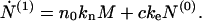
To quantify the kinetic scheme shown in Fig. 1, we introduce the time-dependent state variables M, N_p, and c, which are, respectively, the number concentration of micelles, p-mer fibrils, and free Aβ monomers. We further introduce two structural parameters: m₀ and n₀. These are, respectively, the numbers of monomers in a micelle and in a nucleus. The time evolution of the system is determined by the numerical values of two kinetic parameters, k_n and k_e. The nucleation rate k_n is the average number of nuclei produced by a single micelle per unit time. The number of monomers in a nucleus may in principle be distributed about the number n₀. However, this initial uncertainty is small in comparison with the large final fibril aggregation number. Thus, in the interest of simplicity, we shall assume that all nuclei consist of n₀ monomers. The elongation constant k_e is the coefficient of proportionality between the number of monomers attached per unit time to each fibril and the concentration c of free Aβ monomers in solution.

The time derivative of the concentration of p-mer fibrils, Ṅ_p, is given by

1

The first term on the right hand side of Eq. 1 describes the creation of the fibrils of size p from those of size p − 1 by monomer binding. The rate of such binding is proportional to the concentration c of monomers. The second term accounts for the reduction in p-mer concentration due to conversion into (p + 1)-mers. The third term describes the generation of n₀-mer nuclei from micelles. Eq. 1 assumes unidirectional fibril growth: monomer binding is irreversible and breaking or merging of fibrils is neglected. Preexisting seeds shall be accounted as an initial condition N_p(t = 0).

The two state variables, c and M, are related according to the principles of thermodynamic equilibrium between monomers and micelles (13). Though generally there is a distribution of micelles with aggregation numbers above the minimal number m₀, we will limit ourselves to a very simple two-state model for micelle formation. In this model all micelles have the same aggregation number m₀, and it can be shown that

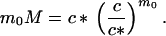2

Here the critical micellar concentration is connected to the free energy of micellization, Δμ⁰, by (14)

where v̄ is the molar volume of water. Both M and c are related to the N_ps by the conservation of mass condition:

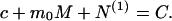3

Here N⁽¹⁾ ☰ ∑ pN_p is the total amount of the protein in fibrillar form.

Eqs. 1–3 constitute a complete set of coupled nonlinear kinetic equations for the variables c, M, and each of the N_p. These equations may be solved and the temporal evolution of the entire fibril distribution N_p(t) may be determined provided that the initial distribution N_p(0) and the total concentration C are known. One can then calculate experimentally observed quantities, such as the scattered light intensity or the distribution of hydrodynamic radii or diffusion coefficients.

Considerable mathematical simplification and physical insight can be achieved by examining the equations governing the temporal evolution of the moments of the fibril distribution. The kth moment N^(k) of the distribution N_p is defined as

4

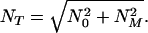
Clearly, the zeroth moment N⁽⁰⁾ is the total number concentration of fibrils of all sizes and the first moment N⁽¹⁾ is the total number concentration of proteins found in all fibrils. Note also that the total intensity of the scattered light is proportional to the second moment N⁽²⁾ of the fibril distribution, provided that the fibril sizes are small compared with the wavelength of light.

Kinetic Equations for the Moments of the Fibril Distribution.

Multiplying all Eq. 1 by p^k and summing, we obtain a set of recursive equations that define the temporal evolution of the kth moment:

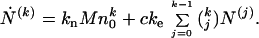5

In this sequence of equations the first two are of particular interest. For the zeroth moment Eq. 5 gives

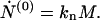6

Here we see that the total number concentration of fibrils changes solely as a result of the process of nucleation from the micelles. For the first moment Eq. 5 gives

7

Here we see that the total number concentration of proteins in fibrillar form changes as a result of both the creation of nuclei (first term on the right-hand side) and the binding of monomers to the ends of each fibril.

Eqs. 6 and 7 together with Eqs. 2 and 3 form a closed set of equations for the four state variables N⁽⁰⁾, N⁽¹⁾, M, and c, which can actually be solved analytically under the condition that m₀ ≫ 1. Furthermore, these two moments provide a clear characterization of the principal features of fibril distribution. In particular, the ratio of these moments gives the average fibril aggregation number

8

Kinetic Evolution of N⁽⁰⁾, N⁽⁰⁾, M, and p̄.

Let us denote the total number concentration of protein in nonfibrillar form as X:

9

Here, if we express M as a function of c according to Eq. 2 we obtain

10

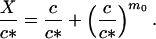
We shall assume that m₀ ≫ 1. Analysis of Eq. 10 shows that in this simple two-state model of micellization either M or c is essentially constant in each of two domains of X, in particular

11

In each concentration domain the relevant Eq. 11 together with Eqs. 3, 6, and 7 forms a complete set of linear equations for variables N⁽⁰⁾, N⁽¹⁾, M, and c, which can be solved analytically.

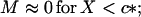
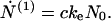
Consider first the case X < c* (regime I)—i.e., low initial concentration of nonfibrillar protein; in this case, M ≅ 0, hence according to Eq. 6, N⁽⁰⁾ remains equal to N₀, the number of fibrils and heterogeneous nuclei (“seeds”) preexisting in the solution at t = 0. Eq. 7 then reduces simply to

12

In this regime N⁽¹⁾ and c are connected according to Eq. 3, by N⁽¹⁾ + c = C. Thus Eq. 12 shows that the concentration c of free monomers decreases exponentially with the time constant (k_eN₀)⁻¹ from its initial value c₀, whereas the amount of protein in fibrillar form grows according to

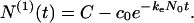13

Because N⁽⁰⁾ remains constant and equal to N₀, the mean aggregation number p̄ = N⁽¹⁾/N⁽⁰⁾ exponentially approaches its final value p̄_f = C/N₀ as described in Eq. 13.

Let as now consider regime II, the case of high initial concentration, X > c*. Here the concentration of monomers remains essentially constant, c = c*, micelles are present, M > 0, and new fibrils are nucleated from micelles. Eliminating N⁽¹⁾ and M in Eqs. 3, 6, and 7 in favor of N⁽⁰⁾ gives the following second-order differential equation:

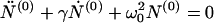14

with γ = n₀k_n/m₀ and ω₀² = k_nk_ec*/m₀. The initial conditions at t = 0 are

15

where N_M is defined as

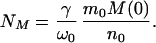16

As we shall see, N_M is the total number concentration of fibrils that would ultimately emerge from micelles in the absence of seeds. Therefore, for C ≫ c*, when most fibrils are nucleated from micelles and the role of seeds is negligible, N_M is related to the final mean aggregation number p̄_f by C = p̄_fN_M. In addition, if C ≫ c*, then at the start of fibrillogenesis C ≅ m₀M(0). Our experiments show dramatic growth of fibrils, i.e., p̄_f ≫ n₀. Hence, m₀M(0) ≫ n₀N_M, and we see from Eq. 16 that γ/ω₀ ≪ 1. Thus we may neglect the second term in Eq. 14, and the solution for N⁽⁰⁾(t), consistent with the initial conditions as given by Eq. 15, may be expressed in the form

17

where

18

and

19

Substituting Eq. 17 into Eqs. 6 and 3, we readily find that

20

Here N⁽¹⁾(0) is the number concentration of protein in the seeds at t = 0. At time T the micelles become exhausted—i.e., M(T) = 0, as can be seen from Eqs. 6 and 17. After this time T no further nucleation occurs and regime II terminates with the final number concentration of fibrils being N⁽⁰⁾(T) = N_T. Thus, according to Eq. 18, when N₀ = 0, N_M is indeed the total number concentration of fibrils in the absence of seeds.

For t > T regime I applies. N⁽⁰⁾ remains equal to N_T and N⁽¹⁾ changes according to Eq. 13 with the starting monomer concentration c₀ being c*, i.e.,

21

We may summarize the evolution of the fibril average aggregation number in the case of high initial concentration, X > c*, by the following expressions. In the domain 0 < t < T

22a

where p̄₀ = N⁽¹⁾(0)/N₀ is the mean number of proteins in a seed. Furthermore, in the domain t > T we obtain p̄(t) by dividing Eq. 21 by N⁽⁰⁾(T) = N_T, hence

22b

According to Eqs. 22b and 18 the final average aggregation number of fibrils is given by

23

We may now make a connection with the qualitative analysis of fibril growth presented previously (12). In that analysis, we assumed X ≫ c* and neglected seeds entirely (N₀ = 0). In that case according to Eq. 23 p̄_f = C/N_M. From the definition of N_M in Eq. 16 we then find p̄_f = n₀ω₀/γ = (m₀k_ec*/k_n)^1/2, as was deduced previously. Also we see from Eq. 19 that when seeds are absent T = π/2ω₀ = (π/2)(m₀/k_nk_ec*)^1/2 regardless of the initial protein concentration. This result coincides with our previous (12) qualitative estimation of T apart from the factor of π/2.

QLS Spectroscopy as a Quantitative Assay for Fibrillogenesis

Relationship Between Aggregation Number and Hydrodynamic Radius for a Single Fibril.

In our experiments we monitor fibril growth using the method of QLS (15, 16). To utilize the theory for the distribution of fibril lengths presented above we must first establish a connection between the dimensions of an individual fibril and its diffusivity as measured by QLS. The diffusion of a fibril is more complex than that of a sphere. For long fibrils whose length L ≥ 1/q, where q is the scattering vector, the temporal autocorrelation function of the scattered light no longer can be represented as a single exponential even for a monodisperse solution (17). Indeed, no explicit analytical expression is available for the autocorrelation function even in the simple case of rigid rods. Nevertheless, it is possible to calculate and measure the first cumulant, ≅ D̄q², and thus determine the mean diffusion coefficient D̄. To calculate the first cumulant we only need to know the form of the diffusion equation for the scattering particles (18). In this work we use the tensor of diffusion coefficients for a cylinder as given by de la Torre and Bloomfield (19) to calculate the first cumulant for a fibril of length L = p/λ and diameter d. Here λ is the number of monomers per unit length of the fibril. We take λ = 1.6 monomers per nm (10, 12).

It is conventional to express the first cumulant in terms of the effective hydrodynamic radius, R_H, according to the Stokes–Einstein relation,

24

Here η is solvent viscosity, T is the absolute temperature, and R_H is the radius of a sphere whose diffusion coefficient is the same as the mean diffusion coefficient of the rigid rod in question. In Fig. 2 we show R_H as a function of p = λL for several relevant values of d and q. As is seen from this figure, the dependence of R_H on p is insensitive to the variations in the fibril diameter or wave vector q within the range of interest. In our calculations we neglected fibril flexibility, which could be characterized by a persistence length of several hundred nanometers (11). This leads to an underestimation of the length of those fibrils that are comparable to, or longer than, the persistence length. This effect could be accounted for by some rescaling of the R_H(p) curve in Fig. 2. It is clear, however, that such rescaling will not impair our ability to assess the effect of variation in solution conditions or in the protein structure on the kinetic constants k_e and k_n. Therefore, for the sake of simplicity we shall model Aβ fibrils as rigid rods and use Fig. 2 as the calibration curve for hydrodynamic radius of a p-mer fibril.

Figure 2.

Calibration curve relating the hydrodynamic radius R_H of a monodisperse solution of rigid rods as a function of the rod length L, or the number of Aβ monomers p. The results are shown for three different rod diameters, d, and for scattering vectors q = 11.8/λ₀, corresponding to 90° scattering in aqueous solution for light having wavelength λ₀ of 633, 514, and 488 nm.

Connection Between Observed Mean Hydrodynamic Radius R̄_H(t) and the Predictions of the Kinetic Theory of Fibrillogenesis.

Knowing the hydrodynamic radius of p-mer, R_H(p), we now can make a connection between the apparent hydrodynamic radius R̄_H determined from the QLS data and the distribution of fibrils N_p which our theory predicts for a particular set of kinetic parameters. Hence we may deduce the kinetic parameters which correspond to the observed evolution of R̄_H. Taking into account the scattering both by micelles and by the distribution of Aβ fibrils with appropriate weighting factors, R̄_H can be related to N_p by

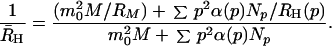25

Here R_M is the radius of a micelle. The contribution of each p-mer fibril is weighted by its scattered intensity, which is proportional to p²α, where α(qL) is the form factor of a rod of length L = p/λ. The corresponding weighting factor for a micelle is m₀². Since a micelle is small, i.e., qR_M ≪ 1, we take its form factor to be unity.

We see from Eq. 25 that, to rigorously apply our kinetic model for the analysis of QLS data, the temporal evolution of the whole fibril distribution function, N_p(t), must be computed numerically. However, if we neglect the polydispersity in the fibril distribution, we can take advantage of the simple analytical theory developed in the previous section. Denoting hydrodynamic radius calculated in this approximation as R̃_H, from Eq. 25 we get

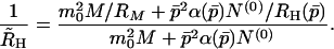26

Here M(t), N⁽⁰⁾(t), and p̄(t) = N⁽¹⁾(t)/N⁽⁰⁾(t) have already been found analytically. As the fibrils grow, the relative contribution of micelles decreases and Eq. 26 reduces simply to R̃_H = R_H(p̄). We now wish to show that, within the accuracy of our experiments, we can replace the rigorous quantity R̄_H by the approximate quantity R̃_H. For this purpose we solved numerically Eqs. 1–3 for N_p(t). We then computed R̄_H according to Eq. 25, using the calibration curve in Fig. 2 for R̄_H(p). The results of this computation for a number of initial concentrations and for a set of kinetic parameters consistent with our experiments are shown in Fig. 3. Here the solid curves represent the time evolution of the apparent hydrodynamic radius R̄_H(t) as computed numerically. They are to be compared with the dashed curves representing the corresponding approximate R̃_H(t) found analytically.

Figure 3.

Temporal evolution of R̄_H(t) (dashed lines) for a polydisperse distribution of fibrils, as computed numerically, and the appropriate R̃_H(t) (solid lines) as calculated using the simple analytic theory for p̄(t), for the following values of the total monomer concentration: curves a, C = 5c*; curves b, C = 0.5c*; and curves c, C = 0.1c*. The parameters of the model used were N₀ = 0.001C, k_n = 2.4 × 10⁻⁶ sec⁻¹, k_e = 90 M⁻¹⋅sec⁻¹, m₀ = 25, c* = 0.1 mM, and n₀ = 10.

Our simplified treatment of monomer–micelle equilibrium neglects the existence of some micelles for X < c*. Consequently, the simple theory underestimates the number of fibrils at low concentration. This leads to overestimation of fibril size. Nevertheless, the difference between the rigorous and the simplified analysis for realistic values of kinetic parameters is significantly less than experimental error. We therefore shall use in further discussions the simple analytical version, since it provides a clear insight into the factors that govern the fibrillogenesis process.

Significance of the Parameters of the Model and Their Deduction from Experimental Data.

The parameters introduced previously can be divided naturally into three groups. The first group consists of structural parameters. These are the linear density λ and the fibril diameter d. The second group of parameters has to do with fibril creation from micelles (c*, m₀, n₀, and k_n) or upon preexisting seeds (N₀). Finally, the parameter k_e describes the rate constant for the binding of monomers to the ends of an individual fibril.

The structural parameters are needed solely to relate the fibril aggregation number p to the length L of a fibril and its observed hydrodynamic radius R_H. The parameters d and λ have been estimated by other workers (10, 12). A readjustment in these parameters would result simply in a rescaling of the calibration curve in Fig. 2. The second group of parameters determines the number of fibrils and therefore the final aggregation number p_f. Knowledge of these parameters facilitates the choice of conditions under which fibrillogenesis can be reproducibly controlled. The nucleation parameters also provide useful information on the intermolecular interactions between Aβ monomers in the micelle. The remaining parameter k_e, which describes the rate of fibril growth, provides insight into the molecular factors that control monomer binding to each fibril end. From a practical viewpoint k_e, is a valuable quantitative measure of the effectiveness of putative growth inhibitors.

We now demonstrate how our theoretical analysis permits an evaluation of the above parameters using the experimental data on R_H reported previously (12). We consider first the simpler case C < c*. Here no additional fibrils are nucleated during fibrillogenesis and the distribution of fibril sizes is determined primarily by the stochastic (Poisson) nature of monomer binding to fibril ends. Thus, the width of distribution N_p(t) grows as , and whatever polydispersity may exist initially in the distribution of seed sizes can be neglected as soon as the fibril size significantly exceeds that of the largest seed. The relative width of distribution decreases in time as 1/p̄^1/2. Under these conditions the mean aggregation number p̄(t) provides a sufficient representation of the extent of fibrillogenesis. We can deduce p̄(t) directly from the experimentally measured mean hydrodynamic radius R_H(t) by using the calibration curve in Fig. 2. The two most useful quantities to be derived from p̄(t) are dp̄/dt at t = 0 and p_f, the fibril final size. With these we can immediately find N₀ and k_e according to N₀ = C/p_f and k_e = (1/C)(dp̄/dt).

We now consider the domain C > c*, where the parameters related to nucleation, namely k_n and c*, play a central role. In this domain micelles are present, and the fibril distribution is the result of a continual emergence of new fibrils from micelles. As we demonstrated above, the fibril distribution, in practice, proves to be sufficiently narrow, so that R̄_H(t) can be satisfactorily represented in terms of p̄(t) and the micellar concentration M(t) by Eq. 26. This equation accounts for the scattering from both micelles and fibrils. As the fibrils emerge and grow in size the micellar contribution to R_H becomes negligible. Then, nearly linear growth of the apparent hydrodynamic radius with time is observed. Here we can again use the calibration curve in Fig. 2 to convert R_H(t) into p̄(t) and thereby determine the rate of fibril elongation, (dp̄/dt) = k_ec*. Since k_e is known from C < c* data, this permits a deduction of the critical micellar concentration c*. Knowing k_ec*, the remaining parameter, k_n, may be deduced from the mean final aggregation number p̄_f (Eq. 23). In the limit C ≫ c* we expect that nucleation within micelles is the dominating source of fibrils, i.e., N_M ≫ N₀, and that practically all the peptide is initially in micellar form: m₀M(0) ≅ C. Under these conditions p̄_f = ((k_ec*(m₀/k_n))^1/2 and hence the ratio k_n/m₀ can be found from p̄_f. An estimation of m₀ can be obtained by comparing the initial (I_i) and final (I_f) values of the scattered light intensity. Because I_i ∼ m₀²M(0) = m₀C and I_f ∼ α(p̄_f)p̄_f²N⁽⁰⁾(∞) = α(p̄_f)p̄_fC, it follows that m₀ = α(p̄_f)p̄_f(I_i/I_f). We found experimentally p̄_f = 480, (I_i/I_f) = (1/7). Using then α(p̄_f) = 0.4 for the form factor, we may estimate that m₀ = 25.

Analysis of our previously reported experimental data (12) produces the following values of the theoretical parameters: k_e = 90 M⁻¹⋅sec⁻¹, c* = 0.1 mM, and k_n = 2.4 × 10⁻⁶ sec⁻¹. Thus, for C > c*, fibrils grow at a rate of 0.5 monomer per min, and new fibril nucleation occurs approximately once in 5 days per micelle. The predicted and the observed temporal evolution of R_H(t) for two samples at C > c* is shown in Fig. 4. In this comparison we used Eq. 26, where p̄(t) is given by Eqs. 22a and 22b. M(t) for t < T is derived by substituting Eq. 17 into Eq. 6. This figure shows that our model successfully represents the essential features of the kinetics of fibrillogenesis. Note that, in the vicinity of the knee of the R_H(t) curve, the experimental points fall below the theoretical prediction. This discrepancy is most likely a consequence of the oversimplified two-state model employed to describe monomer–micelle equilibrium. In fact, the data suggest that there may be a distribution of micellar sizes around the mean aggregate number m₀.

Figure 4.

Comparison between temporal evolution of the samples with Aβ concentration 1.16 mM (A) and 0.47 mM (B) observed experimentally in 0.1 M HCl (+) and calculated using the simple analytic theory (solid curves) with the following parameters: k_n = 2.4 × 10⁻⁶ sec⁻¹, k_e = 90 M⁻¹⋅sec⁻¹, m₀ = 25, c* = 0.1 mM, and n₀ = 10. One percent of the protein was assumed to be in the form of seeds: n₀N₀ = 0.01C.

Conclusions

On the basis of experimental studies using QLS spectroscopy we previously proposed (12) a kinetic model for the in vitro fibrillogenesis of Aβ. According to this model: (i) fibrillogenesis requires the existence of nuclei, which are either produced from micelles of Aβ or are initially present in the solution as seeds; (ii) fibril elongation takes place by the irreversible binding of the monomeric protein to the fibril ends. In the present communication we have presented a detailed mathematical analysis of the model, giving a full description of the temporal evolution of the distribution of the fibril sizes. The theory enables a quantitative deduction of the rate constants for fibril nucleation (k_n), fibril elongation (k_e), and the concentration of seeds (N₀). We have shown that this theory can satisfactorily describe the observed time course of fibrillogenesis for Aβ concentration both below and above c*, the critical concentration for Aβ micelle formation.

This work enables the following advances. First, by combining the experimental method of QLS with the present kinetic theory we obtain a powerful assay method for the quantitative determination of the fundamental kinetic coefficients k_n and k_e, which control fibrillogenesis. Second, the discovery and quantitation of nucleation within micelles gives us means to control the concentration of nuclei that initiate fibrillogenesis. These two advances now place on a solid quantitative footing further examination of the various biochemical and physiologic factors that affect the formation of Aβ fibrils. This knowledge can be highly valuable for the discovery and optimization of pharmacological agents that can inhibit Aβ plaque formation.

ABBREVIATIONS

Aβ

amyloid β-protein

QLS

quasielastic light scattering

References

- 1.Selkoe D J. J Neuropath Exp Neurol. 1994;53:438–447. doi: 10.1097/00005072-199409000-00003. [DOI] [PubMed] [Google Scholar]
- 2.Glenner G G, Wong C W. Biochem Biophys Res Commun. 1984;120:885–890. doi: 10.1016/s0006-291x(84)80190-4. [DOI] [PubMed] [Google Scholar]
- 3.Seubert P, Vigo-Pelfrey C, Esch F, Lee M, Dovey H, Davis D, Sinha S, Schlossmacher M G, Whaley J, Swindlehurst C, McCormack R, Wolfert R, Selkoe D J, Lieberburg I, Schenk D. Nature (London) 1992;359:325–327. doi: 10.1038/359325a0. [DOI] [PubMed] [Google Scholar]
- 4.Narang H K. J Neuropath Exp Neurol. 1980;39:621–631. doi: 10.1097/00005072-198011000-00001. [DOI] [PubMed] [Google Scholar]
- 5.Yankner B A. Neuron. 1996;16:921–932. doi: 10.1016/s0896-6273(00)80115-4. [DOI] [PubMed] [Google Scholar]
- 6.Selkoe D J. Science. 1997;275:630–631. doi: 10.1126/science.275.5300.630. [DOI] [PubMed] [Google Scholar]
- 7.Naiki H, Nakakuki K. Lab Invest. 1996;74:374–383. [PubMed] [Google Scholar]
- 8.LeVine H., III Protein Sci. 1993;2:404–410. doi: 10.1002/pro.5560020312. [DOI] [PMC free article] [PubMed] [Google Scholar]
- 9.Evans K C, Berger E P, Cho C G, Weisgraber K H, Lansbury P T. Proc Natl Acad Sci USA. 1995;92:763–767. doi: 10.1073/pnas.92.3.763. [DOI] [PMC free article] [PubMed] [Google Scholar]
- 10.Shen C-L, Fitzgerald M C, Murphy R M. Biophys J. 1994;67:1238–1246. doi: 10.1016/S0006-3495(94)80593-4. [DOI] [PMC free article] [PubMed] [Google Scholar]
- 11.Shen C L, Murphy R M. Biophys J. 1995;69:640–651. doi: 10.1016/S0006-3495(95)79940-4. [DOI] [PMC free article] [PubMed] [Google Scholar]
- 12.Lomakin A, Chung D S, Benedek G B, Kirschner D A, Teplow D B. Proc Natl Acad Sci USA. 1996;93:1125–1129. doi: 10.1073/pnas.93.3.1125. [DOI] [PMC free article] [PubMed] [Google Scholar]
- 13.Tanford C. The Hydrophobic Effect. New York: Wiley; 1980. [Google Scholar]
- 14.Missel P J, Mazer N A, Benedek G B, Young C Y. J Phys Chem. 1980;84:1044–1057. [Google Scholar]
- 15.Chu B. Laser Light Scattering: Basic Principles and Practice. Boston: Academic; 1991. [Google Scholar]
- 16.Clark N A, Lunacek J H, Benedek G B. Am J Phys. 1970;38:575–585. [Google Scholar]
- 17.Maeda T, Fujime S. Macromolecules. 1984;17:1157–1167. [Google Scholar]
- 18.Akcasu A Z. Polymer. 1981;22:1169–1176. [Google Scholar]
- 19.de la Torre J G, Bloomfield V A. Q Rev Biophys. 1981;14:81–139. doi: 10.1017/s0033583500002080. [DOI] [PubMed] [Google Scholar]