Water-like solvation thermodynamics in a spherically symmetric solvent model with two characteristic lengths

Abstract

We examine by molecular dynamics simulation the solubility of small apolar solutes in a solvent whose particles interact via the Jagla potential, a spherically symmetric ramp potential with two characteristic lengths: an impenetrable hard core and a penetrable soft core. The Jagla fluid has been recently shown to possess water-like structural, dynamic, and thermodynamic anomalies. We find that the solubility exhibits a minimum with respect to temperature at fixed pressure and thereby show that the Jagla fluid also displays water-like solvation thermodynamics. We further find low-temperature swelling of a hard-sphere chain dissolved in the Jagla fluid and relate this phenomenon to cold unfolding of globular proteins. Our results are consistent with the possibility that the presence of two characteristic lengths in the Jagla potential is a key feature of water-like solvation thermodynamics. The penetrable core becomes increasingly important at low temperatures, which favors the formation of low-density, open structures in the Jagla solvent.

In addition to its unique properties as a pure liquid (1–4), water is a remarkable solvent. Of particular interest is its behavior with respect to apolar solutes, which underlies phenomena as diverse as the environmental fate of many pollutants, biological membrane formation, surfactant micellization, and the folding of globular proteins (5, 6). The thermodynamic signatures associated with this “hydrophobic hydration” include negative entropies of transfer of apolar solutes into water at low temperatures, which are only partially compensated by favorable transfer enthalpies (7). Both of these quantities exhibit a pronounced temperature dependence. At sufficiently high temperatures, the roles of entropy and enthalpy are reversed; unfavorable enthalpies of transfer are then only partially compensated by favorable transfer entropies. The resulting solubilities of small apolar solutes therefore exhibit a distinctive minimum with respect to temperature, observed to occur in the 310- to 350-K range.

Because of the important contribution to the driving force for the folding of globular proteins made by the burial of hydrophobic residues (6), the “liquid hydrocarbon” picture of protein folding provides a useful framework for understanding temperature effects on protein stability. Key to this approach is the analogy between the transfer of an apolar solute from a pure apolar phase into water and the exposure of hydrophobic residues upon protein unfolding. There results a common thermodynamic framework for the description of heat and cold denaturation (8, 9) of proteins, the nonmonotonic temperature dependence of the solubility of apolar solutes in water, and the minimum with respect to temperature in the critical micelle concentration of ionic and nonionic surfactants.

There exists a large and important body of theoretical and computational work addressing hydrophobic hydration phenomena (e.g., refs. 7 and 10–26), which we do not attempt to summarize here. Among existing theories of hydrophobic hydration, information theory (IT) (e.g., refs. 13–16) focuses on the relationship between the probability of cavity formation in water, resulting from microscopic density fluctuations, and the hydration free energy corresponding to the transfer of a hard-sphere solute from an ideal gas to bulk water. Assuming that the microscopic density fluctuations obey Gaussian statistics (14, 16), one obtains the following estimate for the solute's chemical potential:

where β = 1/k_BT (k_B is Boltzmann's constant), μ_s^ex is the difference between the solute's chemical potential in water and in an ideal gas at the same density, ρ is water's number density, v is the cavity volume, and σ² = 〈n²〉 − 〈n〉² is the variance of the number of water molecules n in a cavity of size v. For macroscopic cavity volumes, this variance is directly related to the isothermal compressibility K_T, σ² = ρ²vk_BTK_T. Thus, assuming Gaussian statistics and also that the relationship between σ² and K_T holds for microscopic cavities, IT provides an estimate of the hydration free energy from knowledge of water's density and compressibility. This approach has been used to make accurate predictions of the hydration free energies of noble gases and methane as a function of temperature (16).

Traditionally, the modeling of water-like anomalies has placed the emphasis on the role of orientation-dependent interactions [hydrogen bonds (e.g., refs. 27 and 28)] and on the resulting tendency of water molecules to adopt a low-density local structure in which each molecule is on average surrounded by four tetrahedrally arranged nearest neighbors. Recently, it was shown that a family of spherically symmetric potentials consisting of a hard core and a linear repulsive ramp [Jagla model (29–31)] can be tuned so as to seamlessly span the range of behavior from hard spheres to water (32, 33). The Jagla ramp potential contains two characteristic lengths: the hard-core and soft-core diameters a and b, respectively (see Methods). Their ratio is a sensitive control parameter that modulates fluid-phase properties between the hard-sphere and water-like cases. In particular, it was found that there exists a narrow range of values for the ratio of length scales over which the ramp system (32, 33) exhibits a water-like cascade of structural, transport, and thermodynamic anomalies (34). The Jagla model resembles other spherically symmetric potentials that have been used to study water (35, 36).

It has long been known that some water-like anomalies can appear in spherically symmetric systems (e.g., refs. 30, 31, and 37–42). However, the recent realization that these anomalies are sensitively controlled by the existence of two characteristic lengths raises the question of whether a range of other water-like behavior can be reproduced by such two-length spherically symmetric potentials. Given the Jagla fluid's water-like density and compressibility (31–33, 43), one would expect, based on IT predictions, water-like solvation thermodynamics in this fluid. We note, however, that neither the validity of equating microscopic variance and bulk compressibility nor the statistics of microscopic particle number fluctuations have been measured in the Jagla fluid. Furthermore, our study extends also to polymeric hard-sphere solutes, for which Eq. 1 is not valid because of the breakdown of the Gaussian model (17).

In this article, we investigate the solvation properties of ramp solvent molecules whose interaction potential is supplemented with an attractive tail, with respect to apolar solutes. We find that the ramp solvent exhibits key signatures of water-like hydrophobic hydration, namely solubility minima with respect to temperature for hard-sphere solutes, and low-temperature swelling of a hard-sphere chain of possible relevance to the phenomenon of cold denaturation (8, 9, 23, 44). The penetrable core of the Jagla fluid becomes increasingly important at low temperatures, favoring the formation of open structures. Although the mechanism whereby these open structures are formed is different from that in water, the ability to expand upon cooling, common to water and the Jagla fluid, may underlie their similar solvation thermodynamics.

Solubility of Hard Spheres in the Jagla Solvent

We first study the effect of pressure and temperature on the solubility of hard-sphere solutes in the Jagla solvent. To do this, we create a system of N = 1,400 Jagla particles and 2,800 hard spheres of diameter d₀ = a in a box L_x × L_y × L_z with periodic boundary conditions. We fix L_x = L_y = 15a and vary L_z (Fig. 1), maintaining constant pressure and temperature using a Berendsen thermostat (45) and barostat. At sufficiently low temperatures T < T_c1, the mixture of Jagla particles and hard spheres segregates into two phases: Jagla-rich and hard-sphere-rich. For a periodic rectangular simulation cell, the interface forms naturally parallel to face of smallest area. For each pressure and temperature, we equilibrate the system for 10⁴ time units and then measure the mole fraction of hard spheres in a sequence of narrow slabs perpendicular to the z axis during another 10⁵ time units. We find that this equilibration time is larger than the relaxation time of local concentration at all temperatures studied.

Fig. 1.

Explanation of the calculation of the solubility from simulations. (Top) One typical microscopic configuration of a cross-section of the three-dimensional simulation box of dimensions L_x × L_y × L_z with periodic boundary conditions with L_x = L_y = 15a and L_z = 78a. The box contains 1,400 Jagla particles and 2,800 hard spheres. Red spheres represent the hard cores of the solvent particles interacting via the two-scale spherically symmetric Jagla potential, and the green spheres represent hard-sphere solutes. The system is kept at P = 0.3 (> P_c2 = 0.24) and T = 0.9 (> T_c2). (Middle) For the configuration in Top, the instantaneous number of Jagla solvent particles N_J and hard-sphere particles N_S in the slabs of width L_z/100 perpendicular to the z axis. The dashed horizontal line denotes the threshold N₀ = 20 selected to distinguish between the solvent-rich and solvent-lean phases. (Bottom) N_J and N_S averaged over 10⁴ configurations taken over total time of 10⁵ time units. The black solid line shows the derivative |dN_J/dz|, which has a maximum at the boundary between the two phases, denoted here by the gray shaded region, which is excluded from our analysis. Note that N_J and N_S in the solvent-rich and solvent-lean regions are almost constant, as can be seen from the small value of the derivative.

In each slab, we count the numbers N_J of Jagla solvent particles and N_S of hard-sphere solute particles. We define a slab as solvent-rich if N_J > N₀ and as solvent-lean if N_J ≤ N₀, where N₀ is a temperature- and pressure-dependent threshold, such that the slabs form two continuous regions covering the entire system separated by a few slabs corresponding to the interface (see Fig. 1). For convenience, we refer to the slabs as “solvent” in the solvent-rich region and “solute” if solvent-lean, reflecting the fact that, at the conditions investigated here, the coexisting phases are predominantly solvent (Jagla particles) and solute (hard spheres), respectively. The Jagla fluid is clearly a liquid in the solvent-rich phase and vapor-like (i.e., very dilute) in the solvent-lean phase. To exclude boundary effects from the solvent phase analysis, we include only those slabs whose distance to the closest solute slab is >6a. The analogous criterion is applied to the solute phase. Finally, we find the mole fraction of hard spheres in the solvent and solute phases

and compute the ratio

where x_u and x_v are the equilibrium mole fractions of hard spheres in the solute (“u”) and solvent (“v”) phases, respectively. At low enough pressures, k(T, P) becomes Henry's constant, k_H(T), which is the ratio of the solute's liquid-phase fugacity to its liquid-phase mole fraction (46). Under vapor–liquid equilibrium conditions, the solute's fugacity is equal in the vapor and liquid phases. At low enough pressure, the vapor phase behaves like an ideal gas mixture, and the solute's vapor-phase fugacity equals its partial pressure, hence k_H(T) ≈ Px_u/x_v. Thus, knowledge of k_H(T) and measurements of vapor-phase composition allow for the calculation of equilibrium solubilities (46).

Fig. 2 a and b, respectively, shows the calculated solubility x_v as a function of T for P = 0.1, 0.2, and 0.3, and k⁻¹(T, P) for P = 0, 0.1, 0.2, and 0.3. The behavior of the solubility follows that of k⁻¹(T, P), since for T ≪ T_c1, the solvent's vapor-phase mole fraction is very low, and therefore Px_u ≈ P. Hence, x_v ≈ P/k(T, P), and thus the solubility minimum as a function of temperature approximately coincides with the maximum of k(T, P). The striking feature is that, as for apolar solutes in water (47–51), the solubility has a minimum as a function of temperature, here at T_mS = 0.85 ± 0.10, and increases upon cooling below T_mS. Note that the temperature of minimum solubility is considerably higher than the temperature of maximum density, T_MD; for the Jagla liquid, T_MD ≈ 0.5 at P = 0.1 (29, 43, 52). In contrast, the solubility minimum of hard spheres in water occurs close to the TMD (53). Solvation thermodynamics consistent with solubility minima for apolar solutes, as shown in Fig. 2, have also been found in other spherically symmetric water models (36) but only upon using water's experimental ρ(T) relationship. In the present work, the water-like anomalies are inherent in the Jagla model.

Fig. 2.

Simulation results for solubility. (a) The solubility of the hard-sphere solutes in the Jagla solvent as function of temperature (subscript “v” denotes the solvent-rich phase). (b) Symbols indicate our simulation results for 1/k(T, P) = x_v/(Px_u) (see Eq. 3) at four different pressures (subscript “u” denotes the solute-rich phase). 1/k(T, P), in the limit P → 0 coincides with the inverse of Henry's constant 1/k_H(T). The solid line indicates our theoretical prediction based on calculations of thermodynamic mixing quantities (see Eq. 5). Note that x denotes the mole fraction of the solute in the uniform system, whereas x_v denotes the mole fraction of the solute in the solvent-rich phase in equilibrium with the solvent-lean phase. The solubility minimum in a approximately coincides with the minimum of the inverse Henry's constant in b.

Henry's constant can be written as (54)

where v_ℓ is the solvent-phase molecular volume, and μ_s^ex is the difference between the solute's chemical potential in the solvent phase, and in an ideal gas mixture at the same temperature, mole fraction and total density. At sufficiently low pressure, Eq. 4 can be written as

where Δg is the difference, per solute molecule, between the Gibbs energies of the liquid mixture consisting of 1 mole of solute and (1/x − 1) moles of solvent, and the sum of the corresponding pure component liquid-phase Gibbs energies for 1 mole of solute and (1/x − 1) moles of solvent, at the given temperature and pressure. Here, x is the solute mole fraction, and Δs^id = −k_B[ln x + (1/x − 1)ln(1/x − 1)] is the ideal entropy of mixing.

Fig. 2b also shows, as a line, a calculation of 1/k(T, P) using Eq. 5. In summary, the energetic and volumetric contributions to Δg were obtained directly from simulations of the mixture and of the respective hard-sphere and Jagla pure liquids. Thermodynamic integration was used to calculate ΔS. The calculation was performed at a fixed solvent-phase mole fraction, as indicated in the figure. It can be seen that the calculated values of k_H(T) are in good agreement with k(T, P) = Px_u/x_v obtained directly from the phase equilibrium simulations at the same pressure and temperature.

Hard-Sphere Polymer in Jagla Solvent

We next relate the observed solubility minimum of small nonpolar spheres in the Jagla solvent to the degree of extension or collapse of a nonpolar polymer under similar solvent conditions and, correspondingly, to protein pressure- and cold-induced denaturation. If the nonpolar polymer exhibits water-like solution behavior in the ramp solvent, one expects to see a closed loop boundary in the (T, P) plane that encloses the regime of the most compact polymer configurations. The appearance of such a region is also correlated with the appearance of a closed loop region of two phase formation in polymer solutions, with corresponding lower and upper critical solution temperatures.

First, we study the behavior of a relatively short polymer composed of M = 44 monomers modeled by hard spheres of the same diameter as the solute considered above—namely, d₀ = a. We model covalent bonds by linking the hard spheres with the simplest bond potential,

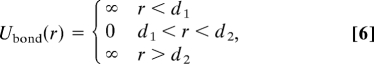so that the minimum extent of a bond is d₁ = a and the maximum extent is d₂ = 1.2a. We simulate for 10⁵ time units the trajectory of the polymer at constant T and P in a cubic box containing N = 1,728 Jagla solvent particles with periodic boundary conditions. We focus on the average polymer radius of gyration R_g(T, P), which is indicative of compact vs. extended configurations.

The behavior of R_g(T, P) has been mapped out and is shown as a function of temperature for six values of pressure in supporting information (SI) Fig. 6. The data are summarized in the diagram in Fig. 3a. For small pressures, R_g(T, P) reaches a very distinct minimum at a temperature denoted as T_mR(P), analogous to hydrophobic polymer collapse in water. T_mR(P) is found to be greater than the temperature for the minimum monomer solubility, T_mR > T_mS(P). As pressure increases, the minimum becomes less pronounced and T_mR(P) shifts to higher temperatures and eventually, at P = 0.4, almost disappears. This pressure-induced swelling behavior is also analogous to that observed in water. From standard polymer theory (55–57), one can also delineate thermodynamic regions where the Jagla solvent is a good solvent, promoting swelling, or a bad solvent, promoting collapse. This theory replaces the complex interactions of the monomers with the surrounding solvent by the effective pairwise interaction potential between monomers and thus does not take into account many aspects of the polymer–solvent interactions such as the possible formation of a vapor-like solvent interface (10) around the completely collapsed globule predicted by a recent theory of hydrophobic hydration (17).

Fig. 3.

Heat and cold polymer unfolding. (a) Contours of equal R_g(T, P) for M = 44 in the P–T plane, showing polymer collapse in the central region of P and T, and reflecting regions of good and poor solvent behavior; the numbers denote the value of R_g(T, P). The large filled circles C₁ and C₂ indicate the liquid–gas and liquid–liquid critical points, respectively. Note that at low P, on decreasing T along a constant P trajectory (dashed line), one passes from a region of good solvent behavior (swollen “denatured” polymers) to a region of poor solvent behavior (collapsed polymers) and finally again to a region of swollen polymer (“cold denaturation”). (b) Schematic illustration of the closed loop region encompassing the domain of hydrophobic collapse for a polymer chain such as studied here, and mimicking the stability regime of native protein folding. In comparison with a, the regions of high-T swelling (“heat denaturation”) and low-T swelling (“cold denaturation”), and the distinct pressure dependence of the polymer melting point are evident in the Jagla solvent model.

Examination of the region of the P–T plane bounding collapsed configurations shows this to have the anticipated closed loop structure. This region lies generally below P_c2 and above the locus of T_MD in the P–T plane. On the high-temperature side, the region where R_g(T, P) < 3.5 is bounded by the liquid–gas critical point. It is noteworthy that the shape of the region of more compact polymer configurations, indicated in Fig. 3b, resembles the typical shape of the regions in the P–T plane in which proteins can fold into their native compact states, although, in the data of Fig. 4a, the transition is gradual (see below).

Fig. 4.

Effect of polymer length M on the swelling behavior at P = 0.1, below P_c2 but above P_c1. Whereas for small M ≤ 88, the temperature dependence of R_g is gradual, consistent with the standard polymer theory, for M = 176, the system exhibits a sharp transition at T ≈ 0.6 between the collapsed state with R_g ≈ 4 and the swollen state with R_g ≈ 10, corresponding to cold swelling (denaturation). Note that R_g of the hard-sphere polymer chain in vacuum coincides approximately with the values of R_g for T ≤ 0.5 for all polymer lengths, indicating that the polymers are in a random coil conformation consistent with dissolution in a “good” solvent.

Interestingly, although the region where the Jagla fluid is a poor solvent for the polymer, corresponding to normal water-like behavior, lies below the critical pressure of the liquid–liquid critical point P_c2, a secondary and distinct solvent behavior is found above P_c2. Although above T_c2, the solvent quality is good and slowly varying over a wide range of temperatures, solvent quality dramatically decreases as we approach T_c2 and presumably cross the Widom line (43, 52, 58). This suggests that the high-density liquid (HDL) in the Jagla model is a poor solvent for the polymer, whereas the low-density, ambient water-like liquid (LDL) is a good solvent for the polymer. This behavior is in accord with expectations based on the anticipated increase in the work of cavity formation in the HDL compared with LDL. The same effect is observed in simulations of water (25).

For protein folding, the transition between compact and extended states is a sharp one. Furthermore, theoretical considerations (10, 17) predict that the interface between water and a large enough apolar solute resembles that between a liquid and its vapor (henceforth referred to as dewetting of the solute). To test the applicability of these aspects of theory to the Jagla solvent, we simulate polymers of increasing numbers of hard-sphere monomers (M = 11, 22, 44, 88, and 176) in the Jagla solvent of N = 4,200 particles at P = 0.1. One can see (Fig. 4) that whereas for M ≤ 88 the dependence of R_g on T is gradual, as expected from the standard polymer theory (55–57), for M = 176 it is almost discontinuous, with a sharp jump from a completely collapsed state with R_g = 4.0a at T = 0.6 to a completely swollen state with R_g = 11.0a at T = 0.3, which is equal to the value of R_g in vacuum.

The solvation of these polymer systems is of interest. However, we note here that the pressure P = 0.1 is above the Jagla fluid's gas–liquid critical pressure, and hence the gaseous phase cannot exist at this pressure for the neat solvent. Hence, the important issue of a true dewetting transition at the polymer–solvent interface (10, 17) cannot be addressed for the thermodynamic states investigated in this work. Preliminary results do indicate the observation of solvent depletion at the polymer globule interface for lower pressures. For completeness, the polymer solvation profiles for several representative cases studied here are reported as SI Fig. 7.

Discussion and Conclusions

We have studied the dissolution of a simple hard-sphere solute, and corresponding polymer, in a two-scale spherically symmetric Jagla solvent previously shown to have water-like liquid properties (29, 31–33, 52). We have found that the system exhibits a temperature of minimum solubility, resembling experimental results in water. In addition, the study of the hard-sphere polymer reveals that the shape of the (T, P) region supporting compact configurations in the Jagla solvent mimics the conventional closed loop region of stable folded protein conformations in water. For large enough polymers, we find a sharp transition between compact and completely collapsed configurations.

Our work is consistent with the possibility of a common physical mechanism in water and the water-like Jagla solvent for the increase of solubility of nonpolar solutes upon cooling (Fig. 2) and, correspondingly, the cold-induced swelling of a polymer. These are engendered by the existence of two repulsive lengths in the model potential, the hard core corresponding to the position of the nearest-neighbor shell of solvent molecules and the soft repulsive core. The latter provides a preference—increasingly significant at low temperature—for a low-density open structure in the solvent. This larger preferred distance, denoted “b” in Fig. 5a, corresponds to the distance preferred by second-neighbor molecules in water, although the forces creating that preference in water have a quite different origin. It is apparently the particular combination of relative distances that, when balanced, leads to remarkably rich water-like behavior in both cases. It is worth noting that the temperature range in which cold denaturation and the solubility minimum occur does not directly coincide with the extrema of other anomalies, such as the temperature of maximum density, which occur at lower temperatures.

Fig. 5.

Model definition and schematic phase diagram. (a) The two-ramp spherically symmetric Jagla potential captures much of the “two-length scale” physics corresponding to the first and the second shells in water (59). The diameter of the hard core r₁ = a = 1 and the diameter of the soft core r₂ = b ≈ 1.72 determine the two-length scales, corresponding to the first and second shells of water. (b) Schematic P–T phase diagram of the two-ramp Jagla model. Shown are the liquid–gas and liquid–liquid critical points (filled circles), the corresponding coexistence lines (dashed lines), the Widom line (solid line), and the locus of temperatures of maximum density labeled T_MD (dashed-dotted line). Along the Widom line, response functions such as the isothermal compressibility and the isobaric heat capacity show maxima (43, 52, 60). LDL and HDL denote the low-density and high-density liquid phases, respectively.

The solvation behavior reported in this work is not accompanied by water-like microscopic structure in the Jagla fluid. At P = 0.1 and T = 0.5 and 0.95 (see Fig. 2), there is no first peak in the pair correlation function at r = a (hard core; see Fig. 5). This feature appears only at higher densities. Hence, there is no first coordination shell with approximately four neighbors, as in water. Another important difference with respect to water is the fact that for P < P_c2, the stable crystal phase of the Jagla potential is a hexagonal close-packed (hcp) lattice (43), which lacks local tetrahedral order. Finally, the liquid–liquid critical point in the Jagla model occurs in the region of the phase diagram where the fluid is stable with respect to crystallization (43), whereas water's second critical point, if it exists, occurs in the region where the liquid is metastable with respect to the crystal (3, 4).

This study suggests several directions for future research. These include the study of solvation thermodynamics of apolar solutes of different sizes in the Jagla solvent, investigation of the solution structure around monomeric and polymeric solutes over broad ranges of temperature and pressure, and a detailed analysis of the energetic and entropic contributions to the solvation free energy of apolar solutes in the Jagla solvent.

Methods

The interaction potential U(r) of the Jagla solvent particles with attractive tail is characterized by five parameters: the hard-core diameter a, the soft-core diameter b, the range of attractive interactions c, the depth of the attractive ramp U_A, and the height of repulsive ramp U_R (Fig. 5) (29). These parameters can be collapsed into three independent dimensionless ratios: b/a, c/a, and U_R/U_A. The ratio of the soft-core and hard-core diameters, b/a, is a sensitive control parameter that, for the purely repulsive case (U_A = 0), determines the fluid's hard-sphere (b/a ∼ 1) or water-like (b/a ∼ 7/4) behavior (33). The latter value of b/a corresponds closely to the ratio of radial distances from a central water molecule to its second- and first-neighbor shells, as measured by the second-nearest and nearest-neighbor peaks of the oxygen–oxygen radial distribution function (≈4.5 and ≈2.8 Å, respectively). Following refs. 29, 43, and 52, we select b/a = 1.72, c/a = 3, and U_R/U_A = 3.5. This choice of parameters produces a phase diagram with several water-like features. It includes two critical points, one corresponding to the first-order liquid–gas transition and the other to a first-order liquid–liquid transition at low temperatures, and a wide region of density anomaly bounded by the locus of temperatures of maximum density (Fig. 5b). The role of the attractive potential, b ≤ r ≤ c, is simply to allow fluid–fluid transitions to occur. Water-like thermodynamic, dynamic, and structural anomalies occur even in the purely repulsive case (U_A = 0), and their appearance is governed by the ratio b/a (32).

The Widom insertion method (58, 61) is the technique of choice to study solvation thermodynamics in the limit of infinite dilution. At nonzero solute concentrations, hence conditions allowing for solute–solute interactions, the standard method for phase equilibrium calculations is the Gibbs ensemble Monte Carlo technique (61, 62). In this article, we adapt to the calculation of phase equilibria a methodology developed in our previous work, the discrete molecular dynamics (DMD) method (42, 45, 63, 64), which has the potential advantage that one does not assume infinite dilution. To use the DMD algorithm, we replace the repulsive and attractive ramps with discrete steps (40 and 8, respectively), as described in ref. 43.

We measure length in units of a, time in units of a(m/U_A)^1/2 (where m is the particle mass), number density in units of a⁻³, pressure in units of U_Aa⁻³, and temperature in units of U_A/k_B. This realization of the Jagla model displays a liquid–gas critical point at T_c1 = 1.446, P_c1 = 0.0417, and ρ_c1 = 0.102, and a liquid–liquid critical point at T_c2 = 0.375, P_c2 = 0.243, and ρ_c2 = 0.370 (43). We model solute particles as hard spheres of diameter d₀. The hard-sphere solutes interact with the Jagla solvent only through excluded volume repulsion, which occurs at the contact distance of (a + d₀)/2. Here, we choose d₀ = a as the hard-core diameter of the Jagla solvent. The dependence of the solubility on d₀ is an important question.

References

- 1.Franks F. Water: A Matrix for Life. 2nd Ed. Cambridge, UK: Royal Society of Chemistry; 2000. [Google Scholar]
- 2.Eisenberg D, Kauzmann W. The Structure and Properties of Water. New York: Oxford Univ Press; 1969. [Google Scholar]
- 3.Debenedetti PG. J Phys Condens Matter. 2003;15:R1669–R1726. [Google Scholar]
- 4.Debenedetti PG, Stanley HE. Phys Today. 2003;56:40–46. [Google Scholar]
- 5.Tanford C. The Hydrophobic Effect: Formation of Micelles and Biological Membranes. 2nd Ed. New York: Wiley; 1980. [Google Scholar]
- 6.Kauzmann W. Adv Protein Chem. 1959;14:1–63. doi: 10.1016/s0065-3233(08)60608-7. [DOI] [PubMed] [Google Scholar]
- 7.Ashbaugh HS, Truskett TM, Debenedetti PG. J Chem Phys. 2002;116:2907–2921. [Google Scholar]
- 8.Privalov PL, Gill SJ. Adv Protein Chem. 1988;39:191–234. doi: 10.1016/s0065-3233(08)60377-0. [DOI] [PubMed] [Google Scholar]
- 9.Privalov PL. Crit Rev Biochem Mol Biol. 1990;25:281–305. doi: 10.3109/10409239009090612. [DOI] [PubMed] [Google Scholar]
- 10.Stillinger FH. J Solution Chem. 1973;1:141–158. [Google Scholar]
- 11.Pratt LR, Chandler D. J Chem Phys. 1977;67:3683–3704. [Google Scholar]
- 12.Dill KA. Biochem. 1990;29:7133–7155. doi: 10.1021/bi00483a001. [DOI] [PubMed] [Google Scholar]
- 13.Garde S, Hummer G, Garcia AE, Paulaitis ME, Pratt LR. Phys Rev Lett. 1996;77:4966–4968. doi: 10.1103/PhysRevLett.77.4966. [DOI] [PubMed] [Google Scholar]
- 14.Hummer G, Garde S, Garcia AE, Pohorille A, Pratt LR. Proc Natl Acad Sci USA. 1996;93:8951–8955. doi: 10.1073/pnas.93.17.8951. [DOI] [PMC free article] [PubMed] [Google Scholar]
- 15.Hummer G, Garde S, Garcia AE, Paulaitis ME, Pratt LR. Proc Natl Acad Sci USA. 1998;95:1552–1555. doi: 10.1073/pnas.95.4.1552. [DOI] [PMC free article] [PubMed] [Google Scholar]
- 16.Hummer G, Garde S, Garcia AE, Paulaitis ME, Pratt LR. J Phys Chem B. 1998;102:10469–10482. [Google Scholar]
- 17.Lum K, Chandler D, Weeks J. J Phys Chem B. 1999;103:4570–4577. [Google Scholar]
- 18.Ashbaugh HS, Garde S, Hummer G, Kaler EW, Paulaitis ME. Biophys J. 1999;77:645–654. doi: 10.1016/S0006-3495(99)76920-1. [DOI] [PMC free article] [PubMed] [Google Scholar]
- 19.Pratt LR. Annu Rev Phys Chem. 2002;53:409–436. doi: 10.1146/annurev.physchem.53.090401.093500. [DOI] [PubMed] [Google Scholar]
- 20.Rajamani S, Truskett TM, Garde S. Proc Natl Acad Sci USA. 2005;102:9475–9480. doi: 10.1073/pnas.0504089102. [DOI] [PMC free article] [PubMed] [Google Scholar]
- 21.Ashbaugh HS, Pratt LR. Rev Mod Phys. 2006;78:159–178. [Google Scholar]
- 22.Athawale MV, Goel G, Ghosh T, Truskett TM, Garde S. Proc Natl Acad Sci USA. 2007;104:733–738. doi: 10.1073/pnas.0605139104. [DOI] [PMC free article] [PubMed] [Google Scholar]
- 23.Tsai C-J, Maizel J V, Jr, Nussinov R. Crit Rev Biochem Mol Biol. 2002;37:55–69. doi: 10.1080/10409230290771456. [DOI] [PubMed] [Google Scholar]
- 24.Widom B, Bhimalapuram P, Koga K. Phys Chem Chem Phys. 2003;5:3085–3093. [Google Scholar]
- 25.Paschek D. Phys Rev Lett. 2005;94:217802. doi: 10.1103/PhysRevLett.94.217802. [DOI] [PubMed] [Google Scholar]
- 26.Paschek D, Nonn S, Geiger A. Phys Chem Chem Phys. 2005;7:2780–2786. doi: 10.1039/b506207a. [DOI] [PubMed] [Google Scholar]
- 27.Poole PH, Sciortino F, Grande T, Stanley HE, Angell CA. Phys Rev Lett. 1994;73:1632–1635. doi: 10.1103/PhysRevLett.73.1632. [DOI] [PubMed] [Google Scholar]
- 28.Truskett TM, Debenedetti PG, Sastry S, Torquato S. J Chem Phys. 1999;111:2647–2656. [Google Scholar]
- 29.Jagla EA. Phys Rev E. 1998;58:1478–1486. [Google Scholar]
- 30.Jagla EA. J Chem Phys. 1999;111:8980–8986. [Google Scholar]
- 31.Kumar P, Buldyrev SV, Sciortino F, Zaccarelli E, Stanley HE. Phys Rev E. 2005;72 doi: 10.1103/PhysRevE.72.021501. 021501. [DOI] [PubMed] [Google Scholar]
- 32.Yan Z, Buldyrev SV, Giovambattista N, Stanley HE. Phys Rev Lett. 2005;95:130604. doi: 10.1103/PhysRevLett.95.130604. [DOI] [PubMed] [Google Scholar]
- 33.Yan Z, Buldyrev SV, Giovambattista N, Debenedetti PG, Stanley HE. Phys Rev E. 2006;73 doi: 10.1103/PhysRevE.73.051204. 051204. [DOI] [PubMed] [Google Scholar]
- 34.Errington JR, Debenedetti PG. Nature. 2001;409:318–321. doi: 10.1038/35053024. [DOI] [PubMed] [Google Scholar]
- 35.Head-Gordon T, Stillinger FH. J Chem Phys. 1993;98:3313–3327. [Google Scholar]
- 36.Garde S, Ashbaugh HS. J Chem Phys. 2001;115:977–982. [Google Scholar]
- 37.Hemmer PC, Stell G. Phys Rev Lett. 1970;24:1284–1287. [Google Scholar]
- 38.Kincaid JM, Stell G. J Chem Phys. 1977;67:420–429. [Google Scholar]
- 39.Stillinger FH, Stillinger DK. Physica A. 1997;244:358–369. [Google Scholar]
- 40.Sadr-Lahijany MR, Scala A, Buldyrev SV, Stanley HE. Phys Rev Lett. 1998;81:4895–4898. [Google Scholar]
- 41.Debenedetti PG, Raghavan VS, Borick SS. J Phys Chem. 1991;95:4540–4551. [Google Scholar]
- 42.Buldyrev SV, Franzese G, Giovambattista N, Malescio G, Sadr-Lahijany MR, Scala A, Skibinsky A, Stanley HE. Physica A. 2002;304:23–42. [Google Scholar]
- 43.Xu L, Buldyrev SV, Angell CA, Stanley HE. Phys Rev E. 2006;74 doi: 10.1103/PhysRevE.74.031108. 031108. [DOI] [PubMed] [Google Scholar]
- 44.Marqués MI, Borreguero JM, Stanley HE, Dokholyan NV. Phys Rev Lett. 2003;91:138103. doi: 10.1103/PhysRevLett.91.138103. [DOI] [PubMed] [Google Scholar]
- 45.Rapaport DC. The Art of Molecular Dynamics Simulation. Cambridge, UK: Cambridge Univ Press; 1997. [Google Scholar]
- 46.Sandler SI. Chemical, Biochemical, Engineering Thermodynamics. 4th Ed. New York: Wiley; 2006. [Google Scholar]
- 47.Harvey AH. AIChE J. 1996;42:1491–1494. [Google Scholar]
- 48.Tsonopoulos C. Fluid Phase Equilib. 2001;186:185–206. [Google Scholar]
- 49.Heidman JL, Tsonopoulos C, Brady CJ, Wilson GM. AIChE J. 1985;31:376–384. [Google Scholar]
- 50.Economou IG, Heidman JL, Tsonopoulos C, Wilson GM. AIChE J. 1997;43:535–546. [Google Scholar]
- 51.Soper AK, Dougan L, Crain J, Finney JL. J Phys Chem B. 2006;110:3472–3476. doi: 10.1021/jp054556q. [DOI] [PubMed] [Google Scholar]
- 52.Xu L, Kumar P, Buldyrev SV, Chen SH, Poole PH, Sciortino F, Stanley HE. Proc Natl Acad Sci USA. 2005;102:16558–16562. doi: 10.1073/pnas.0507870102. [DOI] [PMC free article] [PubMed] [Google Scholar]
- 53.Garde S, Garcia AE, Pratt LR, Hummer G. Biophys Chem. 1999;78:21–32. doi: 10.1016/s0301-4622(99)00018-6. [DOI] [PubMed] [Google Scholar]
- 54.Errington JR, Boulougouris GC, Economou IG, Panagiotopoulos AZ, Theodorou DN. J Phys Chem B. 1998;102:8865–8873. [Google Scholar]
- 55.Flory PJ, Orwoll RA, Virj A. J Am Chem Soc. 1964;86:3507–3514. [Google Scholar]
- 56.Grosberg AY, Khokhlov AR. Giant Molecules. London: Academic; 1997. [Google Scholar]
- 57.Rubinstein M, Colby RH. Polymer Physics. Oxford: Oxford Univ Press; 2003. [Google Scholar]
- 58.Kumar P, Yan Z, Xu L, Mazza MG, Buldyrev SV, Chen S-H, Sastry S, Stanley HE. Phys Rev Lett. 2006;97:177802. doi: 10.1103/PhysRevLett.97.177802. [DOI] [PubMed] [Google Scholar]
- 59.Yan Z, Buldyrev SV, Kumar P, Giovambattista N, Debenedetti PG, Stanley HE. Phys Rev E. 2007;76 doi: 10.1103/PhysRevE.76.051201. 051201. [DOI] [PubMed] [Google Scholar]
- 60.Widom B. J Chem Phys. 1963;39:2802–2812. [Google Scholar]
- 61.Frankel D, Smit B. Understanding Molecular Simulation: From Algorithms to Applications. San Diego: Academic; 1996. [Google Scholar]
- 62.Panagiotopoulos AZ. Mol Phys. 1987;61:813–826. [Google Scholar]
- 63.Alder BJ, Wainwright TE. J Chem Phys. 1959;31:459–466. [Google Scholar]
- 64.Rapaport DC. J Phys A. 1978;11:L213–L217. [Google Scholar]
Associated Data
This section collects any data citations, data availability statements, or supplementary materials included in this article.