A unified framework for linkage and association analysis of quantitative traits

Abstract

We give a unified treatment of the statistical foundations of population based association mapping and of family based linkage mapping of quantitative traits in humans. A central ingredient in the unification involves the efficient score statistic. The discussion focuses on generalized linear models with an additional illustration of the Cox (proportional hazards) model for age of onset data. We give analytic expressions for noncentrality parameters and show how they give qualitative insight into the loss of power that occurs if the scientist‘s assumed genetic model differs from nature's “true” genetic model. Issues to be studied in detail in the future development of this approach are discussed.

A principal goal in both experimental and human genetics is the identification of DNA polymorphisms that play a role in determining measurable phenotypes. These polymorphisms are called quantitative trait loci, or QTL. Unlike experimental genetics, where controlled breeding experiments allow one to map genes by a comparatively direct study of the correlation of phenotypes with the genotypes of markers linked to QTL, human genetics requires different approaches. The two most popular methods are (i) association, or population based mapping, and (ii) linkage, or family-based, mapping. In association mapping, one correlates directly phenotypes and genotypes of genetic markers, in principle, much like the corresponding process in experimental genetics. However, because of population history, which cannot be controlled and which is poorly understood, success using this approach requires the approximate validity of difficult to verify assumptions. In addition to uncertain assumptions about the mode of inheritance of the trait, because of the large number of generations in the history of most populations, the marker location on a chromosome must be very close to the relevant QTL to ensure that recombination over the population history has not severed the connection between QTL and marker. Genome-wide association studies to search for anonymous genes typically use hundreds of thousands of markers to represent the ≈3 × 10⁹ base pairs of a human genome. This marker density has only recently become achievable through the technological advances of high throughput genotyping platforms.

Family-based linkage analysis is based on the assumption that observed similarities in phenotypes of related individuals are caused by similarities in their genotypes at loci influencing those phenotypes. Because this approach depends on family relationships going back only a few generations, there are usually fewer questionable assumptions, and the small number of generations separating pedigree founders from the present means that markers can be much more widely spaced, with perhaps 1,000–10,000 sufficient to cover a human genome with little loss of information. The indirect logic of family based linkage mapping is usually thought to result in a lower signal to noise ratio at an “ideal” marker, and when one combines this with the added complication of recruiting and studying appropriate pedigrees, association studies are increasingly thought to be the method of choice.

Although association and linkage studies usually proceed from similar genetic models, with few exceptions the appropriate statistical methods have been developed along separate lines. In this paper, we provide a unified statistical framework and indicate how it can allow one to study and compare different experimental designs under various conditions. The discussion here is necessarily abstract and simplified. In particular, we mention only in Discussion the issues of multiple testing that arise in genome-wide searches for anonymous genes, we assume that genetic markers are completely informative, and we discuss computational issues only briefly and problems of missing data not at all.

Generally speaking, there are three sources of information for making inferences about the presence of a QTL: the phenotypic measurements, the genotypes of the founders of pedigrees, and the process of inheritance that distributes these genotypes among the nonfounders. The major difference between linkage and association mapping is the way the founder genotypes are treated. In association mapping one models penetrance of the genotypes and uses this model directly in the formation of the test statistic. In linkage analysis, the founder genotypes are used only indirectly, to provide information about the inheritance patterns, which are the sole genetic component used for inference.

Our basic model, described in detail below, is a direct generalization of the model introduced by Fisher (1), who represented phenotypic measurements as sums of genetic and environmental effects and showed the important role of genetic and environmental variance components in relating genotypic to phenotypic variability. He also laid the foundation for family based genetic mapping by computing the phenotypic correlation between relatives.

A weak link in the development of this model is the need to hypothesize a conditional probability distribution of the phenotypes, given the genotypes. To mitigate this problem we will base our approach on the conditional distribution of genotypes given phenotypic values. This insures that conclusions will be relatively robust against model failure with respect to false positive errors, although not necessarily with respect to power to detect true genetic effects. It is also effective in mitigating the effects of nonrandom ascertainment as, e.g., when pedigrees are selected through a proband having a disease related to the phenotype.

In The Efficient Score, we produce score statistics for generalized linear models (GLM) and for the Cox regression model for age of onset phenotypes (2). The key ingredient is a suitable derivative of the log-likelihood with respect to the parameter of interest, evaluated at the null value of that parameter. In the case of association mapping, the first derivative is used. In the case of linkage mapping, the second derivative is used because the first derivative vanishes. It is shown that, in both cases, the test statistic is of the form of a linear combination of the genetic information, weighted by terms that depend on the phenotype and nuisance parameters of the model. In the case of association mapping, the sum is taken over all subjects and the genetic information enters in the form of an hypothesized effect of the genotypes. In the case of linkage mapping, the sum extends over all pairs of subjects and the genetic information enters in the form of centered identity-by-descent relationships. (It turns out that, under the null hypothesis of no linkage and no association, these two efficient scores are uncorrelated, so could be used simultaneously if this seemed advisable.) In Calculating the Variance, we assess the variance of these statistics, and in Nuisance Parameters and Latent Covariates, we propose an algorithm for the estimation of nuisance parameters.

The Noncentrality Parameter is concerned with evaluation of the noncentrality parameter (the expectation of the test statistic when a QTL is present), which is the key in evaluating the power to detect a QTL. It is shown that in association mapping the magnitude of this parameter is determined by the correlation between the true model of penetrance and the assumed one, so the power of association mapping may be greatly affected by a mis-specification of the model. In linkage analysis, however, the noncentrality parameter is much less sensitive to a mis-specification of the model. This and other issues are discussed in Discussion.

Notation

Let Y be an n × 1 vector. The components Y_i denote the phenotypic measurement for subject i. These individuals exist within pedigrees, which can be a single pedigree of size n, n pedigrees of size one, or anything in between. To relate the distribution of Y to a set of genetic and nongenetic covariates, let t be a genomic locus that is to be tested as a QTL. Genetic variability is introduced as an assignment of a pair of haplotypes to each of the pedigrees' founders. We model the haplotypes among founders as independent of each other. These haplotypes are transmitted to the rest of the pedigree in a process summarized by the inheritance vector, which has two coordinates for each nonfounder, each coordinate coded as 0 or 1, the first coordinate to indicate whether the individual's maternally inherited allele comes from the maternal grandmother or grandfather, and the second coordinate to describe similarly the paternally inherited allele. The haplotype assignment of the founders is identified by g_t and the inheritance vector by v_t. Denote by Q_i = Q(v_t(i), g_t) the relevant combination of alleles at the locus in the ith subject, coded as a row vector. The matrix Q, which has n rows, will be called the QTL covariate. In reality, because the exact nature of the QTL is typically unknown, one introduces a possibly different coding of the observed haplotypes as a substitute. We will call the coding for a given subject U_i. For simplicity of the exposition, it is assumed to be a scaler, although vector coding can be used in all that follows. The n × 1 vector U with coordinates U_i will be called the local genetic covariate. We assume that the locus under consideration is within a relatively short genomic subinterval that is unlikely to experience recombination in the meiotic events that define the inheritance vector. Consequently, we may assume that Q and U are direct functions of the pair (v_t, g_t) and that Q_i and U_i correspond, respectively, to the true and to an hypothesized coding. (In general, t can be a vector if we want to model explicitly multiple, possibly interacting genetic loci; but for simplicity we restrict our formal discussion to the case of a single locus. In addition, the location of the QTL will usually be unknown, but again for simplicity we assume at present that Q and U both model the same genetic locus.)

The relation between U and Y will be our primary interest. However, other factors may affect the distribution of the phenotype. The observable factors will be treated as fixed and will be coded in a matrix z. Latent genetic factors will be coded in a matrix G, which we call the global genetic covariate and assume is unlinked to and in linkage equilibrium with the tested locus t. This will be the case if, as we assume, the population is randomly mating. Environmental and other latent nongenetic effects are introduced in a matrix E. We treat both G and E as random effects and assume that they are independent. The combined effect of the covariates on the distribution is assumed to be given by the linear predictor

where β = (β_z, β_U, β_G, β_E) is a vector of regression coefficients. Without loss of generality, we assume that the latent covariates G and E are standardized to have mean zero and unit variance. We will also assume that there is a true model, of the same form as Eq. 1, but with Uβ_U replaced by Qβ_Q.

Remark 1.

In the simple case of a biallelic marker with alleles B and b, an additive coding of U_i is simply the total number of say B alleles in the genotype: 2, 1, or 0. A nonadditive coding would allow the possibility that the coding for the heterozygote Bb differ from the average of the two homozygotes. To consider a range of possible values, one would introduce a second coordinate to U_i, so β_U would become a two dimensional vector. If there are more than two alleles, e.g., if one considers haplotypes or a multiallelic QTL, a saturated model would require high dimensional coding. Consequently, an important issue is the loss of information that occurs if a simple model for U_i fails to capture adequately the complexity of the true covariate Q_i.

In the spirit of GLM (2), we assume a a log-likelihood of the phenotypic measurement associated with subject i in the form ℓ_i(β) = [Y_i θ_i − ψ(θ_i)]/φ, where φ is a scale parameter and ψ is the cumulant generating function with respect to the natural parameter of the exponential family. The parameter θ_i is itself a function of the vector of parameters β and of the covariates via the link function h and the linear predictor: θ_i(β) = h(η_i(β)). We assume that the phenotypic measurements are conditionally independent, given the covariates, so the log likelihood for a sample of size n, conditional on the covariates, both observed and unobserved, takes the form:

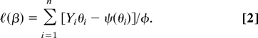In general, the sample will contain pedigrees, within which the genotypic covariates are correlated and the environmental covariates may also be correlated, whereas these covariates are usually regarded as independent between pedigrees. However, the conditional log likelihood can be written in the form of Eq. 2 in all cases. Because the joint distribution of the covariates does not involve the unknown parameters of the model, the conditional likelihood in Eq. 2 is also the full likelihood. In the special case that h(x) = x, ψ(θ) = θ²/2, and φ = σ_e², the phenotype Y is conditionally normally distributed with mean value θ and variance σ_e².

To illustrate the generality of our approach, we also consider the Cox regression model (2), where the “phenotype” is Y_i = (X_i, δ_i), i = 1, …, n, with X_i being the minimum of an age of onset (or survival time) and a censoring time, and δ_i is the indicator that the subject was not censored. The partial log-likelihood takes the form:

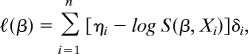where S(β, X_i) = n⁻¹Σ_j∈i e^{η j}, with _i = { j: X_j ≥ X_i}, the group of subjects at risk at time X_i, the age of onset or censoring of the ith individual.

In principle all phenotypes are observable, whereas many covariates are not. We assume henceforth that the fixed-effect covariate z is observable, as is, to an extent made more precise below, the local genetic covariate U. Inference is based on marginal and conditional likelihoods of the observable covariates. Marginal likelihoods can be calculated as conditional expectations, given the observed variable, of the full likelihood. For example, if we assume that we observe the measurements Y and the covariates z and U, then the marginal log-likelihood of β with respect to these observations will be denoted by

(Dependence on the fixed covariates z has been suppressed.) The conditional log-likelihood of the genetic covariate, given the phenotypes (and nongenetic observed covariates), is

To have a better understanding of the relations between association and linkage mapping we consider the inheritance vector v_t and the genotypes among the founders, g_t. In association mapping, the exact form of the genetic variability contributing to the phenotype is modeled, say, in a form of a biallelic DNA variant. Accordingly, the U_i values are observable and inference may be based on the log-likelihoods (Eq. 3). In linkage analysis one assumes that g_t is not available for purposes of inference and restricts consideration to the log-likelihood

which, as we see below, allows inferences based only on inherited genetic relationships among the members of pedigrees. Note that the expectation in the first term of Eq. 4 is now taken with respect to the random distribution of g_t, as well as the other unobserved covariates, conditional on the inheritance vector.

The Efficient Score

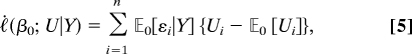
The efficient score, which can be standardized to produce the score statistic for testing the contribution of the locus t to the trait, is formed by taking derivatives of the log-likelihood function with respect to the coefficient β_U and setting the value of that coefficient equal to zero (3). In what follows β₀, and where no confusion can result simply a subscript of 0, will indicate that the vector β has been evaluated at (β_z, 0, β_G, β_E).

For association mapping, we obtain by differentiating Eq. 3 the efficient score

where

and the superscript in parentheses denotes differentiation with respect to the argument of the indicated function. The product form results from the fact that under the null distribution (β_U = 0) the triplet (Y, G, E) is independent of U. The resulting statistic is a linear combination of the centered local genetic covariates. The coefficients are functions of the phenotypes, global covariates, and parameters that must be estimated.

In the special case of a normally distributed response Y with the identity link and φ = σ_e² one obtains ε = [Y − η(β₀)]/σ_e². Suppose the distribution of η(β₀) is normal with mean zβ_z and covariance matrix R. Then Y is normally distributed with mean zβ_z and covariance matrix Σ = R + σ_e²I. By standard multivariate calculations, one sees that the conditional distribution of ε given Y is also normal with mean Σ⁻¹(Y − zβ_z) and covariance matrix R − RΣ⁻¹R. Hence, the efficient score (Eq. 5) is equal in this case to (Y − zβ_z)Σ′⁻¹(U − 𝔼₀|U|). If our sample contains pedigrees, the polygenic random effect G is often assumed to make an additive contribution, which produces a covariance matrix of the form Σ_G = β_G²Φ, where Φ is the matrix of kinship coefficients. In the absence of environmental covariances, one has R = Σ_G. Some details of the calculations in the normal case are given in supporting information (SI) Text.

For linkage mapping, when we take the first derivative of Eq. 4 with respect to β_U and evaluate it at β_U = 0, we find that

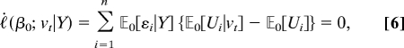whenever the distribution of g_t is exchangeable and v_t involves no inbreeding; in particular whenever there is random mating. Consequently, we use the second derivative and obtain

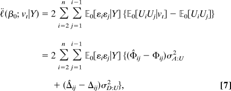where σ_A:U² is the additive variance of the genotypic values of U (see refs. 1 and 4) σ_D:U² is the dominance variance, Φ is the kinship coefficient matrix, and Δ is the matrix with (i, j)th element equal to the probability that individuals i and j share 2 alleles identical by descent (IBD). The entry Φ̂_ij is the proportion of alleles shared IBD at the locus t for the given pair of subjects and Δ̂_ij is the indicator that the pair have inherited two alleles IBD. This statistic is a function of the pairwise IBD relations of the subjects.

Remark 2.

The efficient score as second derivative arises statistically because the likelihood of v_t contains no information about the effect of β_U on the phenotype of an individual, but does carry information about the effect of β_U² on the covariance of phenotypes of related individuals, so the likelihood is properly parameterized by β_U². Mathematically the appearance of the second derivative amounts to the observation that, if a function f(x) can be written as a function of x², say g(x²), then by the chain rule, the first derivative of f with respect to its argument evaluated at x = 0 vanishes, whereas the second derivative of f (evaluated at x = 0) is proportional to the first derivative of g with respect to its argument evaluated at x = 0. For the purposes of this paper we find it more useful to take the second derivative than to reparameterize the likelihood function.

Remark 3.

The claim in the introduction that the efficient scores for linkage and for association are uncorrelated under β₀ follows from consideration of the conditional expectation of the product of the two scores given Y and v_t. The score for linkage is a function of these variables, so comes outside the conditional expectation; the remaining conditional expectation is 0 by Eq. 6.

In the special normal case introduced above, when the marker U has additive genotypic values, one finds that

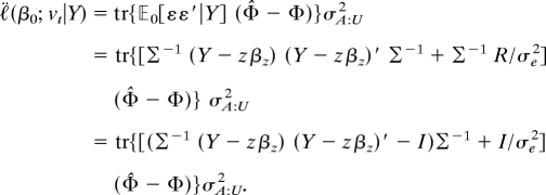The second term in the final line equals tr[Φ̂ − Φ] = 0. Hence, up to a constant factor, this expression reduces to the efficient score proposed by Tang and Siegmund (5) and others (6, 7). See SI Text for details and a generalization to nonadditive coding for U.

For the Cox partial likelihood, we find for association the efficient score

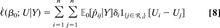where p̂_ij = p̂_ij(β₀) = e^{η j(β0)}/[Σk∈i e^η_k(β0)], j ∈ _i. For linkage, the first derivative of the efficient score vanishes. The second derivative is given in SI Text. Despite its algebraic complexity, the efficient score has again the form of a linear combination of the pairwise IBD relations, with coefficients depending on the responses and on the statistical model for the response.

Calculating the Variance

The efficient scores for testing association are described in Eq. 5 for the generalized linear models and in Eq. 8 for the Cox regression model. The statistics are a linear combination of the vector U − 𝔼₀(U) in the case of generalized linear models and of pairwise differences of the elements of this vector in the case of Cox regression. To use these quantities to test for association, we standardize them by the square root of estimators of their (conditional) variances calculated under the parameter β₀ (3). The covariance matrix of the vector U is

Hence the conditional variance, given Y, of the efficient score (Eq. 5) is

where ε̂ = 𝔼₀(ε|Y). For the Cox regression model one should consider the n² × n² covariance matrix involving

The variance of the efficient score (Eq. 8) is obtained by summing up these covariances multiplied by the appropriate cross products of the linear coefficients.

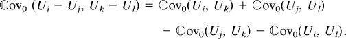
In the case of the efficient score for linkage observe that

The general form of the efficient score in Eq. 7 is a quadratic form, with coefficients depending on the phenotype and on the statistical model used. The variance of the statistic is a sum of pairwise products of weights and the covariances between the different pairwise IBD counts. To write it compactly, it is convenient to use the vec notation to arrange the elements of a matrix into a vector column by column, so

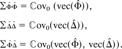Observe that the covariance matrices can be computed by knowing the relatedness of the different members of the pedigrees. Letting ŵ denote the vec of the matrix with entries 𝔼₀(ε_iε_j|Y) from Eq. 7, we have

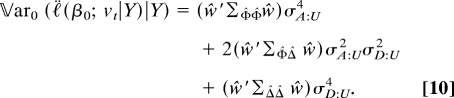Nuisance Parameters and Latent Covariates

The phenotype-dependent coefficients appearing in the efficient scores and in their (conditional) variances involve unknown parameters and the latent covariates G, E. To deal with these we must (i) estimate the nuisance parameters and (ii) calculate appropriate functionals of the conditional distribution of the predictor η, given the response Y. Assuming that we have solved the second task, the first one can be carried out by using either maximum-likelihood estimation, which involves the maximization of Eqs. 3 or 4, or by a least-squares approach, which involves minimization of the variances considered in the previous section. In the normal case, these two are equivalent.

Exact computation of functionals of the conditional distribution of η given Y that appear in the efficient scores may be quite complicated, so it is useful to consider approximations. Recall that η(β₀) = zβ_z + Gβ_G + Eβ_E. Suppose we model the distribution of η(β₀) to be Gaussian with mean zβ_z and covariance matrix R = R(β_G, β_E), where the structure of the covariance matrix, as a function of β_G and β_E reflects our knowledge and beliefs regarding the effect of the within pedigree relations and the environment on the trait. Based on this assumption regarding the marginal distribution of η, one can see that up to an additive term, which does not involve η, the conditional log-likelihood of η, given Y, is equal to

where ℓ(β₀) is specific to the generalized linear model or the Cox regression model.

If the response Y is also normally distributed with the identity link function, the conditional distribution of η, given Y is normal with mean zβ_z + RΣ⁻¹(Y − zβ_z) and covariance matrix R − RΣ⁻¹R. In the case when the response is not Gaussian, one may produce an explicit Gaussian approximation of the conditional distribution by taking a quadratic expansion of ℓ(β₀) with respect to η and completing the squares. Alternatively, instead of attempting to find explicit results, one may employ the Metropolis algorithm to produce random draws from the required conditional distribution. Averaging the evaluations of the vector of linear coefficients as a function of η over the random draws will produce an approximation of the conditional mean.

Except in the normal case, the estimation procedure outlined here can be quite complicated. Even in the normal case, it can become complicated if, as occurs in many linkage studies, pedigrees are not randomly sampled, but are ascertained through one or more probands. See refs. 8 and 9 and the references given there for a more complete discussion.

The Noncentrality Parameter

The power to detect a QTL depends on many factors that complicate the comparisons of different methods. The primary determinant is the noncentrality parameter, i.e., the asymptotic expected value of the score statistic when there is a local genetic factor. Some of the secondary considerations are discussed below.

We simplify the following discussion by assuming (i) that the generalized linear model and the Cox regression model are roughly correct and (ii) that the various nuisance parameters can be estimated without error. [In family-based linkage analysis using an assumed normal model, it is known (9) that, under weak conditions on the structure of the pedigrees, replacing the nuisance parameters by n^1/2-consistent estimates does not affect the noncentrality parameter, and this appears be true in other contexts as well.] These simplifications allow us to focus on what we believe is an important and rarely discussed ingredient in evaluating the noncentrality parameter, namely the the adequacy of the model of the local genetic covariate U, which is often taken to be biallelic and additive. Recall that, in our development of the score tests for association and linkage, we used U as a substitute for the true but unknown factor Q. When U is additive, β_U is scalar. We denote by λ the log-likelihood under the true model, which uses Qβ_Q instead of Uβ_U, so in this section, β = (β_z, β_Q, β_G, β_E) [and β₀ = (β_z, 0, β_G, β_E)]. Without loss of generality, we assume that λ has been standardized to satisfy λ(β₀; Qβ_Q; Q|Y) = 0.

Observe that the conditional expectation given Y of any standardized test statistic Z under a local alternative determined by β_Q may be approximated to the first order by taking the linear term in the Taylor series of λ around β_Q = 0. By virtue of the functional form of λ and of ℓ, this leading term is ℓ̇(β₀; Qβ_Q|Y). Hence, because exp(x) ≈ 1 + x and 𝔼₀(Z) = 0,

If ℓ̇ is identically 0, as it is for family based linkage analysis (cf. Eq. 10), one may use a quadratic expansion to obtain

Consider first the the association statistic, say Z_a, which equals

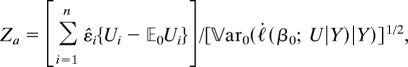where the denominator is given by Eq. 11. Hence, the first-order approximation of the (conditional) noncentrality parameter is

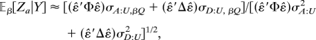where σ_A:U,βQ is the additive covariance between Qβ_Q and U and σ_D:U,βQ the dominance covariance. Observe that ε̂′Φε̂ and ε̂′Δε̂ are determined by structure of the pedigrees, the phenotypes, and the null distribution of the model. Given Y, these terms are constant weights. In the simplest case that no individuals in the sample are related, then Φ and Δ are the identity matrix. In the special case that the original assumed model is correct, σ_A:U,βQ = σ_A:U²β_Q and similarly for σ_D:U,βQ, so β_Q factors out of the quadratic form in the numerator.

If one wants to use the noncentrality parameter as a consideration of experimental design before observing the data, one can under general sets of conditions appeal to the law of large numbers to replace the conditional expectation given Y by the (asymptotic) unconditional expectation under an assumed model, which need not be the same as the model on which the statistic is based. In this way one can also study robustness of the asymptotic noncentrality parameter to violations of the assumed model. If the assumed model is indeed correct, the coefficient of β_Q is the square root of the Fisher information, as one expects from general large sample statistical theory (2).

The asymptotic noncentrality parameter depends on the additive and dominance correlations between U and Qβ_Q. Maximum noncentrality is achieved if these correlations equal one, and the power will be compromised if the correlations are small. A similar result, albeit for different weights, holds for the Cox regression model.

We now turn to the linkage score statistic, say Z_l, and recall that its general form is

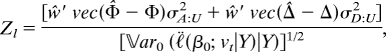where the denominator is given by Eq. 10. Because ℓ̇(β₀; Qβ_Q|Y) vanishes, the leading term in the approximation of the noncentrality is obtained from the correlation of the statistic with the quadratic term in the Taylor series for λ. After taking expectations with respect to the distribution of haplotypes among pedigree founders the approximation becomes

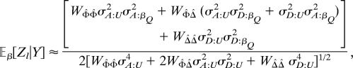where W_Φ̂Φ̂ = ŵ′ ΣW_Φ̂Φ̂ŵ, W_Φ̂Δ̂ = ŵ′Σ_Φ̂Δ̂, and W_Δ̂Δ̂ = ŵ′ Σ_Δ̂Δ̂ŵ.

As above, given the pedigree structure and the phenotypes Y, the W terms are conveniently regarded as fixed constants, which could be simplified under more specific assumptions. If the assumed model is indeed correct, β_Q² can be factored out of the numerator; and under general conditions that permit an application of the law of large numbers the remaining fraction is again asymptotically the square root of the Fisher information. Note also that even if σ_D:U² = 0, i.e., there is no attempt to model dominance, the dominance variance σ_D:βQ² nevertheless appears in the noncentrality paramter. (This is not true for association analysis.)

Because, in linkage mapping, the linear term in the expansion vanishes, there is an apparent reduction in the noncentrality parameter, a fact that in one form or another has been noticed by many and is the basis for the belief that linkage mapping is less efficient than association mapping. As we have observed the approximation is asymptotic to ‖β_Q‖² for linkage and to ‖β_Q‖ for association, and because we have already assumed that ‖β_Q‖ is small in our asymptotic analysis, its square is smaller still. However, one may also observe that linkage analysis is relatively robust to an incorrect assumed model about the mode of inheritance of the QTL. For the linkage statistic, reduction in the noncentrality parameter results from failing to give the right weights to the additive and dominance variances in the formation of the statistic, whereas the noncentrality of the association statistic depends on the correlation between U and Qβ_Q, which is usually much more sensitive to the exact mode of inheritance of the QTL, as the following example shows.

Remark 4.

One may easily construct biallelic examples where the additive variance of Q is zero, whereas the dominance variance is positive. Similarly, one can construct examples where two genes interact to affect the phenotype, but each gene has no marginal effect. In these cases a simple biallelic-additive model for U will result in a noncentrality of zero. However, as follows from our noncentrality calculations in the first case and has been pointed out in refs. 5 and 10, a family-based linkage statistic for the same model will have a nonzero (although not maximal) noncentrality. One can also modify the example of ref. 11 concerning allelic heterogeneity. Suppose there are more than two alleles at a single locus affecting the trait with one allele in complete linkage disequilibrium with allele B of a biallelic marker, whereas another has the same relation with b. If these trait alleles have (additive) effects α₁ and α₂ and occur with frequencies p₁ and p₂ (whereas other alleles have no effect on the trait), and if p₁α₁ + p₂α₂ = 0, the correlation of Q and U is zero, so the simple association statistic has zero noncentrality. Again the linkage statistic will have nonzero noncentrality. These examples are admittedly extreme and there are different strategies for mitigating their effects. But the point remains that, although association studies offer great promise, they are more sensitive than family based linkage studies to the inadequacy of necessarily simplified models in approximating the unknown underlying genetic reality.

Discussion

We have introduced a unified method of statistical analysis for population based association studies and pedigree based linkage studies to map QTL. Our method uses suitable conditional score statistics, given the phenotypic values, which makes the analysis robust with respect to false positive errors. The generality of our model and unified method of analysis make it relatively simple to compare the noncentrality parameters of the two statistics to determine conditions under which one statistic might be preferable to the other, and to examine conditions where the simplifying assumptions commonly used in the definition of the local genetic covariate may lead to substantial loss of power. In particular, we have shown by example and by examining relevant explicit formulae that association studies are less robust than linkage studies with respect to violations of the assumed mode of inheritance. The efficient scores for association and for linkage are uncorrelated, so by squaring and adding the two standardized statistics, one obtains a two degree of freedom statistic that may be more powerful than either statistic individually.

A class of issues we have not discussed are those associated with genome wide searches for anonymous DNA variants. In general a QTL and nearby marker loci will not be at exactly the same genetic locus. In addition to the adequacy of the genetic models, the power of association mapping depends on the linkage disequilibrium between QTL and marker loci, whereas the power of family based linkage mapping depends on the recombination fraction. In both cases the noncentrality parameter at the marker is reduced by the correlation of the (observed) value of the test statistic at the marker and its (unobserved) value at the QTL. Because the effects of linkage disequilibrium usually extend over much shorter genomic distances than those of recombination, many more markers are required to achieve adequate power in association mapping. Consequently, the threshold required to achieve an acceptable false positive error rate is higher in association than in linkage mapping. This also affects comparisons of power.

One can consider multiple, possibly interacting QTL by letting t denote a vector of genetic loci and by taking partial derivatives with respect to the coordinates of t to obtain efficient scores. Detailed calculations will reinforce the relatively greater robustness of linkage statistics compared with association statistics.

The assumption of random mating is stronger than is required for family based linkage analysis. It would suffice for the population to be composed of subpopulations, within which random mating occurs, with no or little mating across subpopulations. In this case quantities such as σ_A:U² and σ_D:U² would in principle vary from one subpopulation to another, which would make various formulas somewhat more complicated, but would not change any essential features of the analysis. With regard to association analysis, if the population is not randomly mating, there may be problems of spurious association, which can lead population based association tests to have unacceptably large false positive rates, unless one can identify randomly mating subpopulations correctly and stratify the analysis accordingly. Family-based association tests (e.g., refs. 12 and 13) ameliorate this problem, but can lead to a loss of power.

Although the discussion in this paper has been entirely conceptual, one point is perhaps worth making with regard to computational algorithms for implementation. For linkage mapping in pedigrees, given a suitable program for estimating identity by descent from marker data (e.g., ref. 14) perhaps complemented by Monte Carlo methods to take care of large pedigrees, calculation of the score statistic is much simpler than calculation of the likelihood ratio statistic for the same model, because segregation parameters are estimated under the null model, β_U = 0, and only once, not at each marker. Consequently, one can use general statistical programming languages and extend the methods more easily to complex models incorporating, for example, gene–gene or gene–covariate interactions.

References

- 1.Fisher RA. Trans R Soc Edinburgh. 1918;52:399–433. [Google Scholar]
- 2.McCullagh P, Nelder JA. Generalized Linear Models. New York: Chapman & Hall; 1999. [Google Scholar]
- 3.Cox DR, Hinkley DV. Theoretical Statistics. New York: Chapman & Hall; 2000. [Google Scholar]
- 4.Kempthorne O. An Introduction to Genetic Statistics. New York: Wiley; 1957. [Google Scholar]
- 5.Tang H-K, Siegmund D. Biostatistics. 2001;2:147–162. doi: 10.1093/biostatistics/2.2.147. [DOI] [PubMed] [Google Scholar]
- 6.Putter H, Sandkuijl L, van Houwelingen J. Genetic Epidemiol. 2002;22:345–355. doi: 10.1002/gepi.01104. [DOI] [PubMed] [Google Scholar]
- 7.Wang K, Huang J. Genet Epidemiol. 2002;23:398–412. doi: 10.1002/gepi.10203. [DOI] [PubMed] [Google Scholar]
- 8.Szatkiewicz JP, T. Cuenco K, Feingold E. Am J Hum Genet. 2003;73:874–885. doi: 10.1086/378590. [DOI] [PMC free article] [PubMed] [Google Scholar]
- 9.Peng J, Siegmund D. Ann Hum Genet. 2006;70:1–15. doi: 10.1111/j.1469-1809.2006.00286.x. [DOI] [PubMed] [Google Scholar]
- 10.Tang H-K, Siegmund D. Genet Epidemiol. 2002;22:313–327. doi: 10.1002/gepi.01108. [DOI] [PubMed] [Google Scholar]
- 11.Siegmund D, Yakir B. The Statistics of Gene Mapping. Berlin: Springer; 2007. [Google Scholar]
- 12.Abecasis GR, Cardon LR, Cookson WO. Am J Hum Genet. 2000;66:279–292. doi: 10.1086/302698. [DOI] [PMC free article] [PubMed] [Google Scholar]
- 13.Rabinowitz D, Laird N. Human Heredity. 2000;50:211–223. doi: 10.1159/000022918. [DOI] [PubMed] [Google Scholar]
- 14.Abecasis GR, Cherny SS, Cookson WO, Cardon LR. Nat Genet. 2002;30:97–101. doi: 10.1038/ng786. [DOI] [PubMed] [Google Scholar]
Associated Data
This section collects any data citations, data availability statements, or supplementary materials included in this article.