Refinement of the x-ray structure of the RC–LH1 core complex from Rhodopseudomonas palustris by single-molecule spectroscopy

Abstract

A unique combination of single-molecule spectroscopy with numerical simulations has allowed us to achieve a refined structural model for the bacteriochlorophyll a (BChl a) pigment arrangement in reaction center–light-harvesting 1 core complexes of Rhodopseudomonas palustris. Details in the optical spectra, such as spectral separation and mutual polarizations of spectral bands, are compared with results from numerical simulations for various models of the BChl a arrangement that were all well within the 4.8-Å limit of the accuracy of the available x-ray structure. The experimental data are consistent with a geometry where 15 BChl a dimers, each taken homologous to those from light-harvesting 2 complex from Rhodopseudomonas acidophila, are arranged in an overall elliptical structure featuring a gap on the long side of the ellipse.

In photosynthesis solar radiation is absorbed by the light-harvesting (LH) apparatus, and the excitation energy is then transferred efficiently to a reaction center (RC), where it is used to create a charge-separated state that ultimately drives all of the subsequent metabolic reactions. Most purple photosynthetic bacteria contain two types of antenna complexes, LH1 complex and LH2 complex (1, 2). The RC is closely associated with LH1, whereas LH2s are arranged around the perimeter of RC–LH1 in a 2D array, the structure of which depends on how the bacteria are grown (3–5). The progress made in high-resolution structural studies of the LH2s (6–9) has strongly stimulated research to understand the detailed mechanisms of the efficient energy transfer processes that take place in these antenna systems. The basic building block of LH2 is a protein heterodimer (αβ), which accommodates three bacteriochlorophyll a (BChl a) pigments and one carotenoid molecule (8). Depending on the bacterial species LH2 consists either of eight or nine copies of these heterodimers, which are arranged in a ring-like structure. It has now been well established that the spatial arrangement of the pigments determines, to a large extent, the spectroscopic features of the complexes and that in these systems collective effects have to be considered to appropriately describe their electronically excited states (10–16). These effects lead to so-called Frenkel excitons, which arise from the interactions of the transition–dipole moments of the individual pigments and correspond to delocalized electronically excited states (17). Because the interaction strength between the individual pigments can be calculated on the basis of the available structural data, information about the pigment arrangement within the LH complexes becomes accessible via optical spectroscopy. From this perspective LH2 has served as a cornerstone for the development of a detailed understanding of structure–function relationships in such antenna systems (18).

In contrast to LH2, where highly resolved x-ray structures are available, the discussion in the literature about the structural properties of RC–LH1 is much more controversial (7, 19–23). Because of the lack of a high-resolution x-ray structure, most proposed geometries are based on low-resolution electron microscopy/atomic force microscopy data (24–28). A detailed discussion on this issue can be found in ref. 18. Here, we focus on the RC–LH1 complex from Rhodopseudomonas palustris for which the first x-ray structure has been determined recently (Fig. 1) (29). In this complex, the RC is enclosed by an overall elliptically shaped LH1 consisting of 15 αβ-apoproteins, each accommodating two BChl a molecules. Interestingly, the LH1 structure features an interruption. Instead of a 16th αβ-apoprotein, another small protein, termed W, has been found that effectively opens the LH1 ring. Unfortunately, the resolution of this structure is only 4.8 Å, and therefore molecular details are insufficiently well defined to allow the precise assignment of the positions and orientations of the BChl a pigments within the complex. Using single-molecule spectroscopic techniques, we have demonstrated that the presence of the physical gap in the RC–LH1 structure of R. palustris produces a gap in the electronic structure of LH1, which leads to severe consequences for the photophysical parameters of the exciton states and the concomitant optical spectra (30).

Fig. 1.

X-ray structure of the RC–LH1 complex from Rps. palustris (29). This structure was determined to a resolution of 4.8 Å. In this complex the RC is enclosed by the LH1, which features 15 αβ (purple and gray) apoproteins that are arranged in an overall elliptical shape and accommodate two BChl a molecules each. The positions and orientations of the BChl a molecules (red) were only placed in the model as guide for the eye. These positions were not absolutely determined at this resolution. The LH1 ring features a gap where one αβ dimer is replaced by another small protein (yellow) that has been termed W. The protein structure representation was prepared with VMD (36).

In this article, we go one step further. Here, we analyze subtle details in the fluorescence–excitation spectra from individual RC–LH1 complexes that would be completely masked in conventional ensemble spectroscopy, because of the large amount of heterogeneity in the samples. These data are compared with results from numerical simulations for various models of the pigment arrangement, i.e., the mutual distance and orientation of the BChl a molecules, within the protein matrix. As a prerequisite for this analysis the tested structures had to be compatible with the x-ray structure, which we used as a starting point. We find the best agreement between the experimental data and the numerical simulations for an equidistant arrangement of 15 BChl a dimers on an ellipse, where the arrangement of the BChl a molecules within a dimer is similar to that of the B850 BChl a molecules in LH2 from Rhodopseudomonas acidophila.

Results

In Fig. 2 we show a comparison of several fluorescence–excitation spectra from RC–LH1 core complexes from Rps. palustris. The top traces show an ensemble spectrum (black) and the sum spectrum (gray) from 41 individual complexes. The ensemble spectrum features a broad band at 11,322 cm⁻¹ with a width of 378 cm⁻¹ (FWHM) and two weak shoulders at 11,545 and 11,655 cm⁻¹, respectively. This spectrum is rather well reproduced by the spectrum that results from summing the 41 individual spectra, indicating that the selected individual complexes are a fair statistical representation of the ensemble. The five lower traces display examples of fluorescence–excitation spectra recorded from individual RC–LH1 complexes. Common to these spectra are variations in the spectral positions and the widths of the observed bands. However, the most striking feature in the spectra from individual core complexes is a narrow spectral line on the low-energy side. As we have shown recently (30), these spectra can be understood on the basis of a simple exciton model for the lowest electronically excited states that takes the physical gap in the BChl a arrangement into account as has been observed in the x-ray structure. The general approach to describe the electronically excited states of the core complexes from Rps. palustris is based on a model Hamiltonian in Heitler–London approximation:

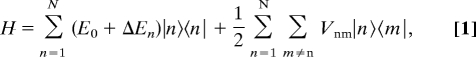where |n〉 and |m〉 correspond to excitations localized on molecules n and m, respectively, (E₀ + ΔE_n) denotes the site energy of pigment n, which is separated into an average, E₀, and a deviation from this average, ΔE_n, and V_nm denotes the interaction between molecules n and m. Accordingly, the electronically excited states of the interrupted LH1 ring become equivalent to a linear excitonic system and, following common practice (17), the exciton states are numbered k = 1, 2, …, 30. The dominant effect of such a gap for the optical spectra is that significant oscillator strength is shifted to the lowest exciton state, i.e., k = 1, in striking contrast to a closed-ring BChl a arrangement where nearly all oscillator strength is accumulated in the next higher exciton states. Because the fluorescence lifetime of the k = 1 state (≈200–300 ps)^§ is rather long with respect to the relaxation of the higher exciton states, which takes place on a ≈100-fs timescale (31, 32), the occurrence of a relatively narrow spectral feature at the red-edge of the absorption spectrum can be well understood.

Fig. 2.

Fluorescence–excitation spectra from RC–LH1 complexes from Rps. palustris. The top two traces show the ensemble spectrum (black) and the spectrum that results from summing 41 spectra from individual core complexes (gray). The lower five traces display fluorescence–excitation spectra from individual RC–LH1 complexes. The spectra have been averaged over all polarizations of the incident radiation. The excitation intensity was 10 W/cm². The vertical scale is given in counted photons per second (cps) and is valid for the lowest trace. The other traces are offset for clarity.

To analyze the spectral bands from the individual core complexes in more detail, we recorded the fluorescence–excitation spectra as a function of the polarization of the incident radiation. The excitation spectra have been recorded in rapid succession, and the polarization of the excitation light has been rotated by 6.4° between each consecutive scans. An example of this protocol is shown in Fig. 3A Upper in a 2D representation where 312 individual scans are stacked on top of each other. The horizontal axis corresponds to photon energy, and the vertical axis corresponds to the individual scans, or equivalently to the polarization of the excitation, and the detected fluorescence intensity is coded by the color scale. The sum spectrum of these scans is presented in Fig. 3A Lower and shows two broad bands at 11,253 and 11,398 cm⁻¹ with a line width of 250 and 153 cm⁻¹ (FWHM), respectively. Again, a narrow feature appears at the low-energy side, which is barely visible in the sum spectrum. In the 2D representation of the data, however, the narrow feature is clearly observable as an intense stripe that undergoes spectral diffusion. The pattern clearly reveals the polarization dependence of the three absorptions, which becomes even more evident in Fig. 3B. Fig. 3B Lower shows two individual scans that have been recorded with mutually orthogonal polarization, where the angle of polarization that yields the maximum intensity for the narrow spectral feature has been set arbitrarily to “horizontal” and provides the reference point. Fig. 3B Upper shows the fluorescence intensity of the three bands as a function of the polarization of the excitation light (red dots, blue dots) and is consistent with a cos² dependence (black). As discussed above, the narrow spectral feature is assigned to the k = 1 exciton transition. Numerical simulations, which will be discussed in more detail below, show that the k = 2 exciton state contributes preferentially to the adjacent broad absorption (at 11,253 cm⁻¹ in Fig. 3B), whereas the other broad band (at 11,398 cm⁻¹ in Fig. 3B) corresponds to a superposition of transitions from exciton states with quantum numbers k ≥ 3. This superposition is also reflected by the curvature of this band in the 2D representation in Fig. 3A, because the mutual orientations of the transition–dipole moments of the higher exciton states vary with respect to each other.

Fig. 3.

Fluorescence–excitation spectrum from an individual RC–LH1 complex from Rps. palustris as a function of the polarization of the excitation light. (A) (Upper) Stack of 312 individual spectra recorded consecutively. Between two successive spectra the polarization of the incident radiation has been rotated by 6.4°. The horizontal axis corresponds to the photon energy, the vertical axis corresponds to the scan number or equivalently to the polarization angle, and the intensity is color-coded. The excitation intensity was 10 W/cm². (Lower) Spectrum that corresponds to the average of the 312 consecutively recorded spectra. (B) (Upper) Fluorescence intensity of the three bands marked by the arrows in Lower as a function of the polarization of the incident radiation (red dots, blue dots) together with cos²-type functions (black) fitted to the data. (Lower) Two fluorescence–excitation spectra from the stack that correspond to mutually orthogonal polarization of the excitation light. The spectra were chosen such that the “horizontal” polarization yielded maximum intensity for the narrow feature at the low-energy side.

In the following, for a better comparison between the experimental data and our simulations, we focus on the data obtained for the k = 1 and k = 2 exciton transitions, because the individual contributions from the k ≥ 3 exciton states to the second broad absorption band vary substantially as a function of the diagonal disorder. For the example shown in Fig. 3 we find for the spectral separation of the k = 1 and k = 2 exciton transitions ΔE = 90 cm⁻¹ and for the respective angle between their transition–dipole moments Δα = 7°. The histograms for ΔE and Δα obtained from 33 individual core complexes are displayed in Fig. 4Middle and Bottom, together with the results from numerical simulations (black squares) that will be discussed in the next section. The histogram for ΔE is centered at 50 cm⁻¹ and has a width of ≈60 cm⁻¹. The distribution for Δα displays a maximum ≈5°, and only very few entries can be found for Δα > 20°, indicating that the transition–dipole moments of the k = 1 and k = 2 exciton states are oriented nearly parallel with respect to each other. A correlation between the values for ΔE and Δα from an individual complex was not observed.

Fig. 4.

Comparison of the energetic separation and the relative orientation of the transition–dipole moments of the k = 1 and k = 2 exciton states from individual RC–LH1 complexes with results from numerical simulations for three different arrangements of the BChl a molecules in the pigment-protein complex. (Top) The model structures A–C that have been used for the numerical simulations. Details are given in the text. Also shown are the model structures B and C on an exaggerated scale to visualize the differences in the pigment arrangement between the two models more clearly. (Middle) Comparison of the experimentally obtained energetic separations between the k = 1 and k = 2 exciton states (gray columns) with numerical simulations (black squares) for the three model structures. (Bottom) Comparison of the experimentally obtained relative orientations of the transition–dipole of the k = 1 and k = 2 exciton states (gray columns) with numerical simulations (black squares) for the three model structures.

To analyze the data in more detail we performed numerical simulations based on the Hamiltonian in Eq. 1. To keep things relatively simple, the average site energies were set to E₀ = 11,570 cm⁻¹ for all pigments and only diagonal disorder, taken randomly from a Gaussian distribution with a width of 100 cm⁻¹ (FWHM), was considered. Further, we omitted off-diagonal disorder and restricted the interaction to nearest-neighbors only. For the different models the only variation that we allowed was the arrangement of the BChl a molecules (within the limits of accuracy of the crystal structure) and the concomitant variation of their interaction strengths. As the simplest approach to evaluate the dependence of the interaction on the distance and the mutual orientation of the pigments we used a dipole–dipole type function (33):

where κ_nm denotes the usual orientation factor, and r_nm denotes the distance between neighboring pigments n and m. The coupling strength V₀ was set to 9.4·10⁴ cm⁻¹·Å³. Accordingly, the proper eigenstates were calculated from diagonalizing the Hamiltonian, which provided the energy, oscillator strength, and orientation of the transition–dipole moment for each exciton state. Each model was run for 3,000 individual realizations of the diagonal disorder.

In model A the mutual orientations and distances of the pigments correspond to the data provided by the protein database that reflects the x-ray structure (see Fig. 4, model A). For this configuration the nearest-neighbor interaction strengths varied considerably around the assembly, i.e., between −70 cm⁻¹ ≤ V_n,n+1 ≤ 230 cm⁻¹ (average 111 cm⁻¹). For models B and C we distributed 15 BChl a dimers on an ellipse with an eccentricity^¶ of ε = 0.5, where each dimer was taken to be homologous to the B850 BChl a dimers in LH2 from Rps. acidophila (8, 34). For model B the dimers were distributed around the ellipse such that their mutual angle was fixed to Φ = 22.5° (see Fig. 4, model B, Φ = const.), whereas for model C the dimers were placed equidistantly around the ellipse, i.e., keeping the length of the arc ds = r_idΦ_i between the dimers on the ellipse constant (see Fig. 4, model C, ds = const.). For model B (model C) the average values for the intradimer and interdimer interaction strengths obtained from Eq. 2 are V_intra = 216 cm⁻¹ (218 cm⁻¹) and V_inter = 125 cm⁻¹ (126 cm⁻¹), respectively. Although for both models the average interaction strengths are about the same, the modulation of the interaction strengths between adjacent molecules differs significantly between models B and C around the ellipse. To illustrate the differences in the pigment arrangement between models B and C, which are barely visible in the three upper images in Fig. 4 Top, the two lower images in Fig. 4 Top show the structures for an eccentricity ε = 0.7 of the ellipse. This exaggeration reveals that for model B the interpigment distance is shortest along the long axis and longest along the short axis of the ellipse and vice versa for model C.

The black squares in Fig. 4 Middle and Bottom show the results of the simulations for the distributions of ΔE and Δα for models A–C together with the experimental data. The simulations based on the structure taken from the protein database (model A) are not able to reproduce the experimental histograms. The simulated distribution for ΔE is significantly broader than that observed experimentally. The simulation is even worse for Δα and yields a bimodal distribution with maxima ≈8° and 43°, which is clearly not compatible with the experimental data. For model B the simulated distribution for ΔE shows a peak at 90 cm⁻¹ (significantly shifted from that of the experimental data) with a width of 62 cm⁻¹. Moreover, the distribution for Δα again shows a bimodal shape with maxima at 23° and 88°. Finally, with model C we calculate for ΔE a distribution that peaks at 50 cm⁻¹ and features a width of 51 cm⁻¹. The distribution predicted for Δα with model C shows a maximum at 0° and decreases rapidly toward larger values. Comparing the three models, it is obvious that neither model A nor model B describes the single-molecule data satisfactorily. Only with model C can we find a reasonable agreement between the simulations and the experimental data. The slight discrepancies still observed between simulation and experiment probably reflect the fact that we used a rather simple exciton model, i.e., equal values for all site energies E₀, restricting the interaction to nearest neighbors and taking only random diagonal disorder into account. Because of space limitations we have restricted the discussion of the model structures to three examples. However, we have tried many more models than those shown here. For structures reminiscent of models B and C, we also shifted the geometrical position of the gap around the ellipse. However, in all of the models tested, only the one with the gap as presented in model C above (i.e., as shown in the x-ray structure, Fig. 1), allowed the simulations to reproduce the essential findings of the experimental data. It is interesting to note that it was relatively simple with all tested model structures to reproduce the ensemble absorption spectrum. Obviously, agreement between a simulated and an experimental ensemble spectrum is a minimum prerequisite that has to be fulfilled by any proposed structural model, but it does not give much insight into the underlying structure of the pigment–protein complexes. In contrast, the use of the detailed single-molecule spectrocopic data provides a much more stringent test of these structural models.

In summary, we conclude that the arrangement of the BChl a molecules in the RC–LH1 complex from Rps. palustris can be modeled adequately by 15 BChl a dimers that are distributed equidistantly around an ellipse and are similar to the dimeric B850 subunit from LH2. Furthermore, successful modeling of the experimental data can only be achieved when the gap in the LH1 ellipse is placed in the same position as that shown in the x-ray structure (Fig. 1). The single-molecule data therefore allow us to propose a refined structural model of the RC–LH1 complex, which is illustrated in Fig. 5.

Fig. 5.

Comparison of the x-ray structure (gray) with the structure used for model C (black). (A) Position and orientation of the BChl a molecules of the RC–LH1 complex from Rps. palustris as taken from the protein database (gray) and from model C (black). (B) Position of the central magnesium ions of the BChl a molecules from the protein database (gray dots) and for model C (black dots). The scale bar indicates the resolution of the x-ray structure. The change in the positions of the magnesium ions in the refined structure are well within the limits of accuracy of the x-ray model.

Methods

Materials.

Trishydroxymethylaminomethane (Tris) and lauryldimethylamine N-oxide (LDAO) were purchased from Sigma–Aldrich. The LH1–RC complexes were isolated and purified from membranes of Rps. palustris as described (29). The complexes were stored at −80°C in 0.05% LDAO, 100 mM Tris·HCl (pH 8.5) buffer until required.

Sample Preparation for the Low-Temperature Experiments.

The stock solution of LH1–RC complexes was highly diluted up to 1·10⁻¹¹ mol. This dilution was performed in detergent buffer [100 mM Tris·HCl (pH 8.5) + 0.05% LDAO]. In the last dilution step 1% (wt/wt) polyvinyl alcohol (PVA; m_W = 124,000–186,000 g/mol) was added. Twenty microliters of the diluted solution was spin-coated onto a lithium fluoride (LiF) substrate by spinning it for 15 s at 500 rpm and 60 s at 2,000 rpm (model P6700, Specialty Coating Systems), producing high-quality amorphous polymer films with <1 μm thickness, in which the pigment–protein complexes are embedded. The samples were immediately mounted in a helium-bath cryostat and cooled down to 1.4 K.

Ensemble and Single-Molecule Fluorescence–Excitation Spectroscopy.

To perform fluorescence–excitation spectroscopy, the samples were illuminated with a continuous-wave tunable titanium–sapphire laser (3900S; Spectra Physics) pumped by a frequency-doubled continuous-wave neodymium/yttrium-vanadate (Nd:YVO₄) laser (Millennia Vs; Spectra Physics) by using a home-built microscope that can be operated either in wide-field or confocal mode. To obtain a well defined variation of the wavelength of the titanium–sapphire laser, the intracavity birefringent filter has been rotated with a motorized micrometer screw, which ensured an accuracy and reproducibility of 0.5 cm⁻¹ for the laser frequency. Fluorescence–excitation spectra of individual LH complexes at T = 1.4 K were obtained as described in detail in ref. 35. Briefly, a (50 × 50)-μm² wide-field image of the sample was taken by exciting the sample at 885 nm and detecting the fluorescence by a back-illuminated, electron-multiplying CCD camera (EMCCD DV887; Andor Technology) after passing suitable band pass filters, which blocked the residual laser light. A spatially well isolated complex was then selected from the fluorescence wide-field image, and a fluorescence–excitation spectrum of this complex was obtained by switching to the confocal mode of the set-up and detecting the fluorescence by a single-photon counting avalanche photodiode (SPCM-AQR-16; EG&G Optoelectronics) while scanning the laser between 840 and 900 nm. The laser was tuned repetitively through this spectral region, and the recorded traces were stored separately. With a scan speed of the laser of 3 nm·s⁻¹ (50 cm⁻¹·s⁻¹) and an acquisition time of 10 ms per data point, this yields a nominal resolution of 0.5 cm⁻¹, ensuring that the spectral resolution is limited by the spectral bandwidth of the laser (1 cm⁻¹). To examine the polarization behavior of the spectra, a λ/2-plate was put in the excitation path. This plate could be rotated in steps of 0.8°, altering the angle of polarization of the excitation light by twice this value.

References

- 1.Zuber H, Cogdell RJ. In: Anoxygenic Photosynthetic Bacteria. Blankenship RE, Madigan MT, Bauer CE, editors. Dordrecht, The Netherlands: Kluwer; 1995. pp. 315–348. [Google Scholar]
- 2.Blankenship RE. Molecular Mechanisms of Photosynthesis. Oxford: Blackwell; 2002. [Google Scholar]
- 3.Scheuring S, Sturgis JN. Science. 2005;309:484–487. doi: 10.1126/science.1110879. [DOI] [PubMed] [Google Scholar]
- 4.Law CJ, Cogdell RJ, Trissl H-W. Photosyn Res. 1997;52:157–165. [Google Scholar]
- 5.Deinum G, Otte SCM, Gardiner AT, Aartsma TJ, Cogdell RJ, Amesz J. Biochim Biophys Acta. 1991;1060:125–131. [Google Scholar]
- 6.Koepke J, Hu X, Muenke C, Schulten K, Michel H. Structure (London) 1996;4:581–597. doi: 10.1016/s0969-2126(96)00063-9. [DOI] [PubMed] [Google Scholar]
- 7.Walz T, Jamieson SJ, Bowers CM, Bullough PA, Hunter CN. J Mol Biol. 1998;282:833–845. doi: 10.1006/jmbi.1998.2050. [DOI] [PubMed] [Google Scholar]
- 8.McDermott G, Prince SM, Freer AA, Hawthornthwaite-Lawless AM, Papiz MZ, Cogdell RJ, Isaacs NW. Nature. 1995;374:517–521. [Google Scholar]
- 9.Papiz MZ, Prince SM, Howard T, Cogdell RJ, Isaacs NW. J Mol Biol. 2003;326:1523–1538. doi: 10.1016/s0022-2836(03)00024-x. [DOI] [PubMed] [Google Scholar]
- 10.Hu X, Ritz T, Damjanovic A, Autenrieth F, Schulten K. Q Rev Biophys. 2002;35:1–62. doi: 10.1017/s0033583501003754. [DOI] [PubMed] [Google Scholar]
- 11.van Amerongen H, Valkunas L, Grondelle V. Photosynthetic Excitons. Singapore: World Scientific; 2000. [Google Scholar]
- 12.van Oijen AM, Ketelaars M, Köhler J, Aartsma TJ, Schmidt J. Science. 1999;285:400–402. doi: 10.1126/science.285.5426.400. [DOI] [PubMed] [Google Scholar]
- 13.Hofmann C, Aartsma TJ, Köhler J. Chem Phys Lett. 2004;395:373–378. [Google Scholar]
- 14.Gerken U, Jelezko F, Götze B, Branschädel M, Tietz C, Ghosh R, Wrachtrup J. J Phys Chem B. 2003;107:338–343. [Google Scholar]
- 15.Mostovoy MV, Knoester J. J Phys Chem B. 2000;104:12355–12364. [Google Scholar]
- 16.Zigmantas D, Read EL, Mancal T, Brixner T, Gardiner AT, Cogdell RJ, Fleming GR. Proc Natl Acad Sci USA. 2006;103:12672–12677. doi: 10.1073/pnas.0602961103. [DOI] [PMC free article] [PubMed] [Google Scholar]
- 17.Knoester J, Agranovich VM. In: Thin Films and Nanostructures. Agranovich VM, Bassani GF, editors. San Diego: Elsevier; 2003. pp. 1–96. [Google Scholar]
- 18.Cogdell RJ, Gall A, Köhler J. Q Rev Biophys. 2006;39:227–324. doi: 10.1017/S0033583506004434. [DOI] [PubMed] [Google Scholar]
- 19.Scheuring S, Francia F, Busselez J, Melandri BA, Rigaud JL, Levy D. J Biol Chem. 2004;279:3620–3626. doi: 10.1074/jbc.M310050200. [DOI] [PubMed] [Google Scholar]
- 20.Scheuring S. Curr Opin Chem Biol. 2006;10:387–393. doi: 10.1016/j.cbpa.2006.08.007. [DOI] [PubMed] [Google Scholar]
- 21.Gerken U, Lupo D, Tietz C, Wrachtrup J, Ghosh R. Biochemistry. 2003;42:10354–10360. doi: 10.1021/bi034969m. [DOI] [PubMed] [Google Scholar]
- 22.Aird A, Wrachtrup J, Schulten K, Tietz C. Biophys J. 2007;92:23–33. doi: 10.1529/biophysj.106.084715. [DOI] [PMC free article] [PubMed] [Google Scholar]
- 23.Frese RN, Olsen JD, Branvall R, Westerhuis WHJ, Hunter CN, van Grondelle R. Proc Natl Acad Sci USA. 2000;97:5197–5202. doi: 10.1073/pnas.090083797. [DOI] [PMC free article] [PubMed] [Google Scholar]
- 24.Karrasch S, Bullough PA, Ghosh R. EMBO J. 1995;14:631–638. doi: 10.1002/j.1460-2075.1995.tb07041.x. [DOI] [PMC free article] [PubMed] [Google Scholar]
- 25.Qian P, Hunter CN, Bullough PA. J Mol Biol. 2005;349:948–960. doi: 10.1016/j.jmb.2005.04.032. [DOI] [PubMed] [Google Scholar]
- 26.Stahlberg H, Dubochet J, Vogel H, Gosh R. J Mol Biol. 1998;282:819–831. doi: 10.1006/jmbi.1998.1975. [DOI] [PubMed] [Google Scholar]
- 27.Scheuring S, Goncalves RP, Prima V, Sturgis JN. J Mol Biol. 2006;358:83–96. doi: 10.1016/j.jmb.2006.01.085. [DOI] [PubMed] [Google Scholar]
- 28.Scheuring S, Busselez J, Levy D. J Biol Chem. 2005;280:1426–1431. doi: 10.1074/jbc.M411334200. [DOI] [PubMed] [Google Scholar]
- 29.Roszak AW, Howard TD, Southall J, Gardiner AT, Law CJ, Isaacs NW, Cogdell RJ. Science. 2003;302:1969–1971. doi: 10.1126/science.1088892. [DOI] [PubMed] [Google Scholar]
- 30.Richter MF, Baier J, Prem T, Oellerich S, Francia F, Venturoli G, Oesterhelt D, Southall J, Cogdell RJ, Köhler J. Proc Natl Acad Sci USA. 2007;104:6661–6665. doi: 10.1073/pnas.0611115104. [DOI] [PMC free article] [PubMed] [Google Scholar]
- 31.Sundström V, Pullerits T, van Grondelle R. J Phys Chem B. 1999;103:2327–2346. [Google Scholar]
- 32.Vulto SIE, Kennis JTM, Streltsov AM, Amesz J, Aartsma TJ. J Phys Chem B. 1999;103:878–883. [Google Scholar]
- 33.Sauer K, Cogdell RJ, Prince SM, Freer AA, Isaacs NW, Scheer H. Photochem Photobiol. 1996;64:564–576. [Google Scholar]
- 34.Matsushita M, Ketelaars M, van Oijen AM, Köhler J, Aartsma TJ, Schmidt J. Biophys J. 2001;80:1604–1614. doi: 10.1016/S0006-3495(01)76133-4. [DOI] [PMC free article] [PubMed] [Google Scholar]
- 35.Hofmann C, Aartsma TJ, Michel H, Köhler J. New J Phys. 2004;6:1–15. [Google Scholar]
- 36.Humphrey W, Dalke A, Schulten K. J Mol Graphics. 1996;14:33–38. doi: 10.1016/0263-7855(96)00018-5. [DOI] [PubMed] [Google Scholar]