Fluctuation and synchronization of gait intervals and gait force profiles distinguish stages of Parkinson's disease

Abstract

We study the effects of Parkinson's disease (PD) on the long-term fluctuation and phase synchronization properties of gait timing (series of interstride intervals) as well as gait force profiles (series characterizing the morphological changes between the steps). We find that the fluctuations in the gait timing are significantly larger for PD patients and early PD patients, who were not treated yet with medication, compared to age-matched healthy controls. Simultaneously, the long-term correlations and the phase synchronization of right and left leg are significantly reduced in both types of PD patients. Surprisingly, long-term correlations of the gait force profiles are relatively weak for treated PD patients and healthy controls, while they are significantly larger for early PD patients. The results support the idea that timing and morphology of recordings obtained from a complex system can contain complementary information.

1. Introduction

Time series of fluctuating, but approximately periodic processes, are studied in many complex natural systems to characterize their control dynamics with methods from statistical physics such as fluctuation analysis and phase synchronization analysis [1,2]. A well-known example is the electro-physiological recording of the heart activity, using the conventional electrocardiogram (ECG). On the one hand, records of interbeat intervals (‘tachograms’) are analyzed to understand and characterize the control exerted by the autonomous nervous system [3–7]. On the other hand, the morphology of the ECG waveforms of each heartbeat (‘morphograms’) contain important information on the physical status of the heart itself [8]. Although derived from the same recordings, both, intervals and morphology have been shown to contain complementary information, e.g., distinguishing healthy subjects from heart failure patients [3–5,7,8].

Gait analysis is used to augment the diagnosis and prognosis of various neurological diseases. For example, it has been shown that increased stride-to-stride variability is associated with Parkinson's disease (PD) [9]. Furthermore, increased gait variability was found to be a risk factor for falls occurring from unknown reasons among elderly people [10,11]. Many gait analysis systems also provide information about the force profile exerted by each foot on the ground during walking. As this represents the temporal pattern of the contact between the foot and the ground, it is hypothesized that force profiles would contain information about the quality of gait. More specifically, the consistency by which foot–ground contact is performed along a given walking path may reflect the level of gait stability.

In this paper, we study recordings of gait force profiles obtained for both legs in PD patients and healthy controls. Similar to the approach for ECG data, we extract and study interstride interval series (corresponding to tachograms in ECGs) and series of stride force profiles (corresponding to morphograms in ECGs). Analyzing both the fluctuation and synchronization behavior of these time series, we find that the information in the data is fully complementary. Fluctuation and phase synchronization analysis of the interstride interval series yield different results for PD and early PD (EPD) patients compared to elderly healthy controls. At the same time, fluctuation analysis of gait force profiles yields similar behavior for treated PD patients and controls, while EPD patients who were not treated with medication differ.

The paper is organized as follows: In Section 2, we describe the database used and the methodology for the extraction of the two types of series from the recordings. We present brief descriptions of the detrended fluctuation analysis (DFA) method and the closely related central moving average (CMA) method which we employed to study the long-term scaling behavior of the fluctuations. Furthermore, a phase synchronization approach is introduced to quantify bilateral synchronization in step timing. Section 3 reports our results for the fluctuation behavior of both types of time series as well as for the synchronization between both legs. We discuss our results and conclude in Section 4.

2. Database and methodology

2.1. Subjects and extraction of time series

PD patients (n = 29, mean age ± standard error: 67.0 ± 1.3 yr) were compared to healthy elderly subjects (n = 24, 64.3 ± 1.3 yr) (‘controls’) and to 13 subjects (68.9 ± 2.3 yr) with de novo PD (early PD: EPD), i.e., patients who were diagnosed as suffering from PD but have not yet been treated with any anti-Parkinsonian medications.¹ The age difference between the three groups was not significant; patients and subjects did not suffer from any other neurological disease.

The subjects wore force-sensitive insoles [14] that recorded with a sampling frequency of 100 Hz the normal force exerted by the floor while stepping during a period of 2 min of comfortable walking. Subjects walked along a 25 m long corridor, turned when they reached an end, and continued walking. The PD patients were examined during the time in which the medication was effective (‘ON’ stage).

In Fig. 1 (a) typical force profiles of both legs are shown for one subject. Beginning and end of stance times (e.g., the duration when the foot is on the ground) are defined by heel-strikes and toe-offs, respectively; stride times are defined as the duration between consecutive heel-strikes of the same leg. To study the data of each subject and each leg, we defined two different time series. First we used the series of time differences ${\tau }_k^{\mathrm{hs},l}=t_{k+1}^{\mathrm{hs},l}-t_k^{\mathrm{hs},l}$ between two consecutive heel-strikes of one leg (l = right [ri] or left [le] leg, hs = heel-strike, see Fig. 1(a)) to determine the fluctuation behavior of stride timing. These series do not contain any information about the shape of the force profiles during stance time. Therefore, we extracted a second time series from the morphology of the gait force profiles in order to study their fluctuations over time. More precisely, we rescaled each profile curve of each stance period to the interval [0, 1]. Furthermore, the rescaled data was normalized in time to a fixed number of L = 64 data points² (see Fig. 1(b)). This process of rescaling and time normalization properly removes biases which are related to the measurement device (e.g., different amplification levels in different insoles), the body weight of the subjects, as well as stride-to-stride variations in stride timing. As one can see in the power spectra of two different force profiles in Fig. 1(c), the lower frequencies (f < 15 Hz³) contain most of the power and are thus more significant for the signal shape. Hence, to characterize the shape of the kth gait force profile, we considered only the spectral power ${\stackrel{‒}{\Phi }}_k^l$ of the frequencies 1 ≤f < 15 Hz, and defined a morphology series $P^l=\left(P_k^l\right)$ (integrated power) by

$$P_k^l=\sum _{1\le f<15\mathrm{Hz}}{\stackrel{‒}{\Phi }}_k^l\left(f\right)$$ (1)

Fig. 1.

(a) Typical force profiles of the right (broken line) and left (solid line) leg during walking. Times of heel-strikes and toe-offs are marked by crosses and circles, respectively. (b) Extracted and rescaled force profile of one step (as indicated by the bold line in (a), crosses) after time normalization. For comparison another rescaled force profile of a different subject is shown (circles). (c) Corresponding power spectra of the normalized force profiles shown in (b).

for both legs, l = ri or le, separately. Note that we did not consider the first Fourier coefficient since $\stackrel{‒}{\Phi }(f=0\mathrm{Hz})$ is only a constant proportional to the mean of the force profile.

Fig. 2(a) shows the normalized histograms of the standard deviations of stride-to-stride times, σ(τ^hs), and Fig. 2(b) shows the normalized histograms of the standard deviations of the morphology series, σ(P), for all three groups.⁴ As one can see, the standard deviations for EPD and PD patients are increased for ${\tau }_k^{\mathrm{hs}}$ and P_k (see also Tables 1 and 2 for a summary and statistical comparison).

Fig. 2.

Normalized histograms of the standard deviations of (a) stride-to-stride times ${\tau }_k^{\mathrm{hs}}$ and (b) the morphology parameters P_k of controls (circles), EPD (triangles) and PD patients (crosses).

Table 1.

Standard deviation and scaling exponents of stride-to-stride time series τ^hs; the values are given as mean ± standard error

	σ(τhs) (s)	αDFA1	αCMA	αDFA1cor
Controls	0.027 ± 0.001a	0.92 ± 0.03b	0.84 ± 0.03c	0.80 ± 0.03c
EPD	0.047 ± 0.007a	0.88 ± 0.05	0.79 ± 0.05	0.73 ± 0.04
PD	0.053 ± 0.013a	0.84 ± 0.02b	0.76 ± 0.03c	0.72 ± 0.03c

Scaling exponents calculated by the DFA1, CMA and corrected DFA1 method are significantly increased for controls compared to PD patients. The scaling exponents of EPD and PD patients are not significantly different.

Mann—Whitney test:

^aControls vs. EPD, Controls vs. PD: P<0.0001.

^bControls vs. PD: P<0.05.

^cControls vs. PD: 0.05<P<0.06.

Table 2.

Standard deviation and scaling exponents for gait force-sensitive time series (the values are given as mean ± standard error)

	σ(P) (a.u.)	αDFA1	αCMA	αDFA1cor
Controls	0.0062 ± 0.0003a,b	0.74 ± 0.02c	0.65 ± 0.01c	0.61 ± 0.02c
EPD	0.0082 ± 0.0008b	0.86 ± 0.03c,e	0.76 ± 0.03c,d	0.70 ± 0.02c,d
PD	0.0099 ± 0.0013a	0.75 ± 0.02e	0.68 ± 0.02d	0.63 ± 0.02d

Scaling exponents calculated by means of DFA1, CMA and corrected DFA1 are significantly larger for EPD subjects when compared to controls and PD patients. The scaling exponents of controls and PD patients are not significantly different.

Mann—Whitney test:

^aControls vs. PD: P = 0.01.

^bControls vs. EPD: P = 0.05.

^cControls vs. EPD: P<0.01.

^dEPD vs. PD: P<0.05.

^eEPD vs. PD: P<0.01.

2.2. Detrended fluctuation analysis (DFA)

A widely used method to study long-term fluctuations and correlations in time series is detrended fluctuation analysis (DFA) [15–18]. In this approach, the time series (x_k), k = 1, ..., N is first integrated, $Y\left(n\right)={\sum }_{k=1}^n(x_k-\langle x\rangle )(\text{with}\langle x\rangle =(1∕N){\sum }_{k=1}^N{x}_k)$. After dividing Y(n) into N_s ≡ [N/s] non-overlapping segments of equal length (scale) s, a piecewise polynomial trend $y_s^v\left(n\right)$ is estimated within each segment v = 1 + [(n − 1)/s] and the detrended series is calculated by

$${\stackrel{\sim }{Y}}_s\left(n\right)=Y\left(n\right)-y_s^v\left(n\right).$$ (2)

The degree of the polynomial can be varied in order to eliminate linear, quadratic or higher order trends of the integrated time series [6]; here we used DFA1 (linear polynomials for detrending). The variance of the detrended series, $F_s^2\left(v\right)=\langle {\stackrel{\sim }{Y}}_s^2\left(n\right)\rangle$, calculated in each segment v, yields the fluctuation function on scale s

$$F\left(s\right)={\left[\frac{1}{N_s}\sum _{v=1}^{N_s}{F}_s^2\left(v\right)\right]}^{1∕2}={\left[\frac{1}{s{N}_s}\sum _{n=1}^{s{N}_s}{\stackrel{\sim }{Y}}_s^2\left(n\right)\right]}^{1∕2},$$ (3)

which—for scaling data—increases with s as $F\left(s\right)\sim s^{\alpha }$ (α is called the scaling or ‘Hurst’ exponent). The asymptotic value α = 0.5 indicates the absence of long-range correlations in the data. If 0.5<α<1.0 the data are long-range correlated, i.e., they are characterized by a power-law decay of the autocorrelation function $C\left(s\right)=\left(\langle x_k-\langle x\rangle \rangle \right)\left(\langle x_{k+s}-\langle x\rangle \rangle \right)\sim s^{-\gamma }$ with γ = 2 − 2α and a power spectrum $P\left(f\right)\sim f^{-\beta }$ with β = 2α − 1 [15,16]. The higher α, the stronger the correlations in the signal.

2.3. Central moving average (CMA) analysis

A possible drawback of the DFA method is the occurrence of abrupt jumps in ${\stackrel{\sim }{Y}}_s\left(n\right)$ (Eq. (2)) at the boundaries of the segments, since the fitting polynomials in neighboring segments are not related. As a simple way to avoid these jumps the central moving average (CMA) method was suggested recently [19] (see also [20], where this method is compared with the backward moving average technique). In CMA, Eq. (2) is replaced by

$${\stackrel{\sim }{Y}}_s\left(n\right)=Y\left(n\right)-\frac{1}{s}\sum _{j=-(s-1)∕2}^{(s-1)∕2}Y(n+j),$$ (4)

while Eq. (3) stays the same. In some cases, the scaling behavior of F(s) vs. s is more smooth for CMA than for DFA, as we see in Fig. 3. Here we used both methods for comparison.

Fig. 3.

Fluctuation functions vs. time scale s after applying DFA1 (left), CMA (middle) and corrected DFA1 (right) of stride-to-stride time series τ^hs of a control subject (circles), an EPD patient (triangles) and a PD patient (crosses). The scaling exponent of each subject was derived by a least square fit of F(s) vs. s in the scaling range 3≤s≤s_max. For the control subject, ${\alpha }_{\mathrm{DFA}1}=0.90,{\alpha }_{\mathrm{CMA}}=0.82,{\alpha }_{\mathrm{DFA}{1}_{\mathrm{cor}}}=0.79$ (with s_max = 20), for the EPD patient, ${\alpha }_{\mathrm{DFA}1}=0.82,{\alpha }_{\mathrm{CMA}}=0.78,{\alpha }_{\mathrm{DFA}{1}_{\mathrm{cor}}}=0.70$ (with s_max = 18) and for the PD patient, ${\alpha }_{\mathrm{DFA}1}=0.77,{\alpha }_{\mathrm{CMA}}=0.68,{\alpha }_{\mathrm{DFA}{1}_{\mathrm{cor}}}=0.65$ (with s_max = 16) (for the sake of clarity, F(s) functions of the PD patient were multiplied by a factor of 1.5).

2.4. Corrected DFA for very short data

It has been shown that conventional DFA and CMA systematically overestimate the scaling exponent α on very small scales [16,21]. This might be a problem for very short time series, where scales s<15 need to be included in the fitting procedure to determine α. As suggested by Kantelhardt et al. [16], a more reliable procedure involves the comparison with the corresponding analysis of shuffled data. Hence, we also consider

$$F_{\mathrm{mod}}\left(s\right)=\frac{F\left(s\right)s^{1∕2}}{{\langle F_{\text{shuff}}^2\left(s\right)\rangle }^{1∕2}},$$ (5)

where ${\langle F_{\text{shuff}}^2\left(s\right)\rangle }^{1∕2}$ denotes the DFA (or CMA) fluctuation function (Eq. (3)) averaged over several configurations of shuffled data, taken from the original series (x_k).

2.5. Synchronization analysis

The methods described above can be used to study the properties of signals derived from each leg separately. In order to focus on the interrelation between both legs, we calculated the degree of phase synchronization between them. Note that we did not filter our data, since bandpass filtering could lead to an overestimation of phase synchronization [24].

First we determined the phase difference between right and left leg via marker events (e.g., heel-strikes [hs] and toe-offs [to]):

$$\Delta {\phi }_k^m=2\pi \frac{t_k^{m,\mathrm{ri}}-t_k^{\mathrm{hs},\mathrm{le}}}{t_{k+1}^{\mathrm{hs},\mathrm{le}}-t_k^{\mathrm{hs},\mathrm{le}}},$$ (6)

where $t_k^{m,\mathrm{ri}}$ refers either to the heel-strike (mode m = hs) or the toe-off point (m = to) of the right leg. This approach is equivalent to the technique of Poincare section, which is a widely used method to analyze chaotic systems [22]. The resulting phase differences typically form a time series $\psi =\Delta {\phi }_1^{\mathrm{hs}},\Delta {\phi }_1^{\mathrm{to}},\dots ,\Delta {\phi }_k^{\mathrm{hs}},\Delta {\phi }_k^{\mathrm{to}},\dots$ with means $\Delta {\stackrel{‒}{\phi }}^{\mathrm{hs}}\ne \Delta {\stackrel{‒}{\phi }}^{\mathrm{to}}$. For the sake of a uniform analysis of $\Delta {\phi }^{\mathrm{hs}}$ and $\Delta {\phi }^{\mathrm{to}}$, we calculated the time series of the normalized phase differences $\stackrel{\sim }{\psi }=\Delta {\stackrel{\sim }{\phi }}_1^{\mathrm{hs}},\Delta {\stackrel{\sim }{\phi }}_1^{\mathrm{to}},\dots ,\Delta {\stackrel{\sim }{\phi }}_k^{\mathrm{hs}},\Delta {\stackrel{\sim }{\phi }}_k^{\mathrm{to}},\dots$ with $\Delta {\stackrel{\sim }{\phi }}_k^{\mathrm{hs}}=\Delta {\phi }_k^{\mathrm{hs}}-\frac{1}{2}(\Delta {\stackrel{‒}{\phi }}^{\mathrm{hs}}-\Delta {\stackrel{‒}{\phi }}^{\mathrm{to}})$ and $\Delta {\stackrel{\sim }{\phi }}_k^{\mathrm{to}}=\Delta {\phi }_k^{\mathrm{to}}+\frac{1}{2}(\Delta {\stackrel{‒}{\phi }}^{\mathrm{hs}}-\Delta {\stackrel{‒}{\phi }}^{\mathrm{to}})$. Plotting the histogram of the normalized phase differences would lead to a single peak in case of high synchronization between both legs. Contrary, an absence of synchronization will show a uniform distribution. To reliably quantify the distribution of phase differences, one can calculate the Shannon entropy $S=-{\sum }_{j=1}^N{p}_j$ ln p_j of the corresponding histogram (p_j is the relative frequency of finding $\stackrel{\sim }{\psi }$ within the jth bin of the histogram and N is the number of bins). An index which measures the degree of phase synchronization is defined by

$$\rho :=\frac{S_{\max }-S}{S_{\max }},$$ (7)

where S_max = ln N is the maximal entropy, meaning a uniform distribution of the phase differences $\stackrel{\sim }{\psi }$ [22]. According to this definition, no synchronization corresponds to ρ = 0 (uniform distribution of $\stackrel{\sim }{\psi }$), whereas ρ = 1 means the distribution is localized in one point (δ-function). The value of ρ strongly depends on the number of bins of the histogram. It is suggested to estimate the optimal number of bins as N = exp[0.626 + 0.4 ln(M − 1)] where M is the number of samples [22,23]. However, to be able to compare our results among all subjects) (with different number of samples) we chose a sufficient number of bins and set N = 100 for all analyses.

3. Results

3.1. Fluctuation analysis of stride-to-stride time series

We analyzed time series of stride-to-stride intervals using DFA1, CMA and the corrected DFA1. For this purpose, we manually removed all data related to the walking turns and calculated the fluctuation function of both legs by F(s)^hs = ([F²(s)^hs,ri + F²(s)^hs,le]/2)^1/2 (cf. Eq. (3)). Fig. 3 depicts results for a typical control subject (circles), an EPD patient (triangles) and a PD patient (crosses). Whereas the scaling exponent of the healthy elderly subject is close to α = 1.0, suggesting strong long-range correlations, the EPD and the PD patients show more random behavior.

The group averages of the scaling exponents are summarized in Table 1. In general, the values obtained for the three methods show the same qualitative behavior. The differences are clearly due to the overestimation of α by DFA1 and—to a much lesser extent—by CMA, while corrected DFA1 consistently yields the smallest and probably most reliable results. The scaling exponents of the controls are significantly higher than for EPD and PD patients. The scaling exponents of EPD patients are higher than for PD, however, the differences are not significant.

To verify our interpretation that the estimated scaling exponents of α>0.5 are due to long-range correlations and not a result of a broad distribution of the data, we shuffled each time series of each leg in each subject and obtained α_shuff ≈ 0.5 in all cases.

We further compared the first and second half of each subject's walk to evaluate the possible role of fatigue. For all subject groups, the mean and SD of the stride time was not different in the two halves (paired T-test, P>0.1), indicating that at least for these parameters, fatigue did not have a strong effect.

3.2. Fluctuation analysis of gait force profile series

As described in Section 2.1, we also extracted form sensitive time series $\left(P_k^l\right)$ to study variations in the gait force profiles with time. Fig. 4 shows results for one typical subject of each group after applying DFA1, CMA and the corrected DFA1 (walking turns were again removed manually). The computed scaling exponents of the EPD subject are clearly increased compared to controls and PD patients, suggesting that the stride-to-stride variability of the ground reaction force does not change monotonously with the progression of the disease.

Fig. 4.

Fluctuation analysis of the form sensitive time series P of a control subject (circles), an EPD patient (triangles) and a PD patient (crosses) by means of DFA1 (left), CMA (middle) and corrected DFA1 (right). The scaling exponent of each subject was derived by a least square fit of F(s) vs. s in the scaling range 3≤s≤s_max. For the control subject one finds ${\alpha }_{\mathrm{DFA}1}=0.73,{\alpha }_{\mathrm{CMA}}=0.66,{\alpha }_{\mathrm{DFA}{1}_{\mathrm{cor}}}=0.61$ (with s_max = 17), for the EPD patient ${\alpha }_{\mathrm{DFA}1}=0.92,{\alpha }_{\mathrm{CMA}}=0.82,{\alpha }_{\mathrm{DFA}{1}_{\mathrm{cor}}}=0.78$ (with s_max = 14) and for the PD patient ${\alpha }_{\mathrm{DFA}1}=0.76,{\alpha }_{\mathrm{CMA}}=0.70,{\alpha }_{\mathrm{DFA}{1}_{\mathrm{cor}}}=0.63$ (with s_max = 14) (for the sake of clarity, F(s) functions of the EPD patient were multiplied by a factor of 1.5).

Table 2 summarizes the results of each subject group, showing that the scaling exponents of EPD are significantly increased when compared to controls and PD patients. Again, the values obtained for the three analysis methods show the same qualitative behavior. All differences between DFA1, CMA, and corrected DFA1 are clearly due to the overestimation of α by DFA1 and—to a lesser extent—by CMA, while corrected DFA1 consistently yields the smallest and probably most reliable results. We also compared all resulting Hurst exponents to those of the corresponding shuffled data. Since α_shuff ≈ 0.5, we can assume that the enhancements in α_DFA1, α_CMA and ${\alpha }_{\mathrm{DFA}{1}_{\mathrm{cor}}}$ are due to long-range correlations in $\left(P_k^l\right)$.

3.3. Phase synchronization analysis applied to stepping periods of either legs

The stepping of each leg can be considered as a periodic process. We assume that the enhanced fluctuations in stride timing in PD and EPD will also effect the level of phase synchronization between left and right leg, since large fluctuations might disturb regular synchronization patterns. However, increased random noise levels might increase phase synchronization in weakly coupled or uncoupled oscillators as studies of model systems recently showed [25]. It is thus interesting to study the phase synchronization between left and right leg in our experimental data.

We estimated the level of phase synchronization by calculating ρ (see Eq. (7)) for controls, EPD subjects, and PD patients. Fig. 5 depicts $\stackrel{\sim }{\psi }$ series taken from one control and one PD subject. It is clear that the variance in $\stackrel{\sim }{\psi }$ is lower for the control subject as compared to the PD patient. Likewise the value of ρ was higher for that subject. As Fig. 5 suggests, control subjects usually performed more walking turns than EPD and PD patients due to higher gait speed. In order to compare ρ-values between the three groups we only considered the values of $\stackrel{\sim }{\psi }$ until the middle of the third interturn interval.

Fig. 5.

The normalized phase differences $\stackrel{\sim }{\psi }$ between both legs are plotted against time for (a) one control subject and (c) one PD patient. Note that data become irregular during turns for both subjects. However, clear increased variation of $\stackrel{\sim }{\psi }$ can be detected in the interturn periods of the PD patient as compared to the control subject. Panels on the right-hand side show the corresponding normalized histograms and ρ-values, (b) for the control subject, and (d) for the PD patient. Turn times of control subject: 14.7, 29.6, 45.0, 59.4, 75.3, 90.1, 105.9 s; turn times of PD patient: 29.8, 62.5, 95.7 s.

Fig. 6 shows the normalized histograms of the synchronization indices ρ for each group. As one can see, synchronization is larger in the group of controls when compared to EPD and PD patients, see also Table 3.

Fig. 6.

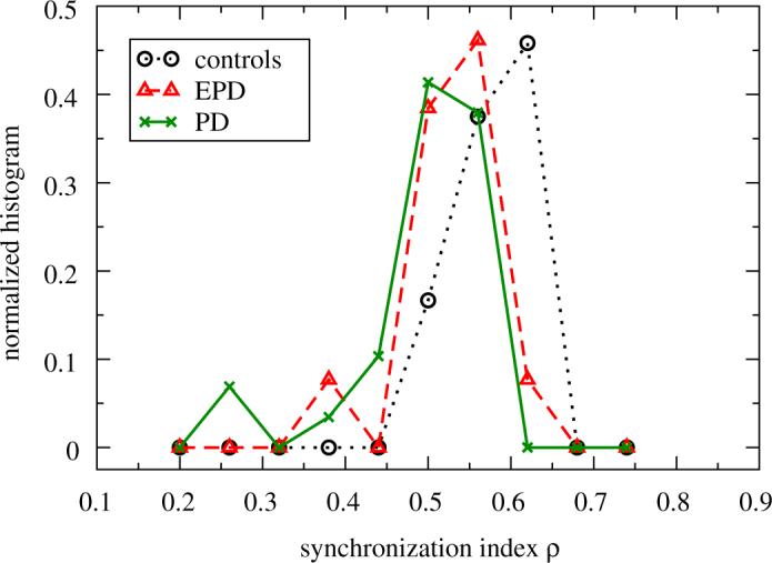
Synchronization index ρ after analyzing the synchronization between right and left leg for controls (circles), EPD (triangles) and PD patients (crosses). The normalized histogram for the controls is significantly different for the EPD and PD patients (see also Table 3). The lines are guides to the eye.

Table 3.

Synchronization index ρ for healthy elderly subjects, EPD and PD patients (the values are given as mean ± standard error)

	ρ
Controls	0.62 ± 0.01
EPD	0.55 ± 0.02
PD	0.53 ± 0.02

The values of ρ for the control group are significantly higher (Mann—Whitney test: P<0.001) when compared to EPD and PD patients.

4. Discussion and conclusions

In this study, we applied statistical physics methods to the investigation of normal and impaired gait. We demonstrated that these methods allow refined examination of the Parkinsonian gait, revealing disturbances not always apparent to the clinical eye.

4.1. Fluctuations in stride-to-stride time series and in the morphology of stepping force profiles

Our results show that PD leads to a more random timing of patient's gait (recall Section 3.1), consistent with previous findings [26,27]. Large values of α indicate persistent gait, i.e., slow steps are followed by relatively slow steps and fast steps by relatively fast steps. This persistence can also be observed in both PD and EPD patients, but it is significantly lower. In addition, the magnitude of the gait timing fluctuations is significantly increased in PD and EPD patients (see σ(τ^hs) in Table 1 and Fig. 2). Both changes indicate alterations in the motor and step-to-step regulation of the stride pattern. Fluctuations in the morphology of stepping force profiles were characterized by scaling exponents that were significantly increased for EPD patients who were not yet treated with any anti-Parkinsonian medication (Fig. 4 and Table 2). This finding is surprising, since the magnitude of the fluctuations, characterized by the standard deviation, is intermediate for EPD patients. As shown in Table 2, the standard deviation σ(P) increases from controls to EPD to PD as does the standard deviation of the interstride intervals (see Table 1). Nevertheless, gait profile morphologies are significantly more persistent in EPD subjects. These results show that the information contained in stride-to-stride intervals and in stride morphology is complementary. One possible explanation for this surprising behavior is that long-term usage of medication attenuates fluctuations in the morphology of gait force profiles, but not fluctuations in gait cycle timing.

4.2. Phase synchronization analysis of the Parkinsonian gait

The decrease of phase synchronization of gait timing in PD and EPD patients is most probably not due to the decreased long-term correlations in common fluctuations, since less correlated common noise, externally imposed on two weakly coupled oscillators, seems to increase phase synchronization, whereas strongly correlated noise suppresses it [28]. The random fluctuations are much stronger in PD and EPD patients than in the healthy controls (see σ(τ^hs) in Table 1 and Fig. 2). Hence, in this example, the noise is likely disturbing the synchronization between the legs rather than causing it. This might suggest that the noise is generated separately in each of two oscillators rather than equally imposed on them externally by a central process. Indeed several recent physiological studies support the hypothesis of motor disassociation between the legs during the walking of PD patients (e.g., Refs. [29,30]).

4.3. Clinical implications

In general, classical medical methods are effective for the purposes of the diagnosis and treatment of PD patients. At the same time, gait disturbances are among those disease implications that may require deeper inspection and evaluation, in particular due to the potential grave consequences that they have on independence, e.g., falls [31,32]. In the present study, by the use of fractal analysis we confirm that long-term gait variability in the timing of generation of consecutive gait cycles is a marker for Parkinsonian gait [33]. More equivocal are the results regarding the variation in the shape of the force profiles. While PD patients untreated with drugs have higher degrees of long-term fluctuations as compared to elderly subjects, PD patients who have longer duration of the disease, show comparable long-term variations in the force profiles to that existing among healthy elderly subjects. This finding warrants further investigations, especially in light of the possibility that when under the influence of the anti-Parkinsonian drugs, foot placement during walking is partially stabilized.

References

- 1.Bunde A, Kropp J, Schellnhuber H-J, editors. The Science of Disasters—Climate Disruptions, Heart Attacks, and Market Crashes. Springer; Berlin: 2002. [Google Scholar]
- 2.Strogatz SH. Sync: How Order Emerges from Chaos in the Universe, Nature, and Daily Life. Penguin Books; Harmondsworth: 2004. [Google Scholar]
- 3.Peng C-K, Mietus J, Hausdorff JM, Havlin S, Stanley HE, Goldberger AL. Phys. Rev. Lett. 1993;70:1343. doi: 10.1103/PhysRevLett.70.1343. [DOI] [PubMed] [Google Scholar]; Peng C-K, Mietus J, Hausdorff JM, Havlin S, Stanley HE, Goldberger AL. Physica A. 1998;249:491. doi: 10.1016/s0378-4371(97)00508-6. [DOI] [PubMed] [Google Scholar]
- 4.Ivanov PC, Rosenblum MG, Peng C-K, Mietus J, Havlin S, Stanley HE, Goldberger AL. Nature. 1996;383:323. doi: 10.1038/383323a0. [DOI] [PubMed] [Google Scholar]
- 5.Ivanov PC, Amaral LAN, Goldberger AL, Havlin S, Rosenblum MG, Struzik ZR, Stanley HE. Nature. 1999;399:461. doi: 10.1038/20924. [DOI] [PubMed] [Google Scholar]
- 6.Bunde A, Havlin S, Kantelhardt JW, Penzel T, Peter J-H, Voigt K. Phys. Rev. Lett. 2000;85:3736. doi: 10.1103/PhysRevLett.85.3736. [DOI] [PubMed] [Google Scholar]
- 7.Ashkenazy Y, Ivanov PC, Havlin S, Peng C-K, Goldberger AL, Stanley HE. Phys. Rev. Lett. 2001;86:1900. doi: 10.1103/PhysRevLett.86.1900. [DOI] [PubMed] [Google Scholar]
- 8.Bartsch R, Henning T, Heinen A, Heinrichs S, Maass P. Physica A. 2005;354:415. [Google Scholar]
- 9.Hausdorff JM, Schaafsma JD, Balash Y, Bartels AL, Gurevich T, Giladi N. Exp. Brain Res. 2003;149:187. doi: 10.1007/s00221-002-1354-8. [DOI] [PubMed] [Google Scholar]
- 10.Hausdorff JM, Edelberg HK, Mitchell SL, Goldberger AL, Wei JY. Arch. Phys. Med. Rehabil. 1997;78:278. doi: 10.1016/s0003-9993(97)90034-4. [DOI] [PubMed] [Google Scholar]
- 11.Hausdorff JM, Rios D, Edelberg HK. Arch. Phys. Med. Rehabil. 2001;82:1050. doi: 10.1053/apmr.2001.24893. [DOI] [PubMed] [Google Scholar]
- 12.Yogev G, Giladi N, Peretz C, Springer S, Simon ES, Hausdorff JM. Eur. J. Neurosci. 2005;22:1248. doi: 10.1111/j.1460-9568.2005.04298.x. [DOI] [PubMed] [Google Scholar]
- 13.Baltadjieva R, Giladi N, Gruendlinger L, Peretz C, Hausdorff JM. Eur. J. Neurosci. 2006;24:1815. doi: 10.1111/j.1460-9568.2006.05033.x. [DOI] [PubMed] [Google Scholar]
- 14.Bäzner H, Oster M, Daffertshofer M, Hennerici M. J. Neurol. 2000;415:841. doi: 10.1007/s004150070070. [DOI] [PubMed] [Google Scholar]
- 15.Peng C-K, Buldyrev SV, Havlin S, Simons M, Stanley HE, Goldberger AL. Phys. Rev. E. 1994;49:1685. doi: 10.1103/physreve.49.1685. [DOI] [PubMed] [Google Scholar]
- 16.Kantelhardt JW, Koscielny-Bunde E, Rego HHA, Havlin S, Bunde A. Physica A. 2001;295:441. [Google Scholar]
- 17.Hu K, Ivanov PC, Chen Z, Carpena P, Stanley HE. Phys. Rev. E. 2001;64:011114. doi: 10.1103/PhysRevE.64.011114. [DOI] [PubMed] [Google Scholar]
- 18.Chen Z, Ivanov PC, Hu K, Stanley HE. Phys. Rev. E. 2002;65:041107. doi: 10.1103/PhysRevE.65.041107. [DOI] [PubMed] [Google Scholar]
- 19.Alvarez-Ramirez J, Rodriguez E, Echeverría JC. Physica A. 2005;354:199. [Google Scholar]
- 20.Xu L, Ivanov PC, Hu K, Chen Z, Carbone A, Stanley HE. Phys. Rev. E. 2005;71:051101. doi: 10.1103/PhysRevE.71.051101. [DOI] [PubMed] [Google Scholar]
- 21.Bashan A, Bartsch R, Kantelhardt JW, Havlin S. Physica A. submitted for publication.
- 22.Rosenblum MG, Pikovsky AS, Kurths J, Schäfer C, Tass PA.Hoff AJ, Moss F, Gielen S.Neuro-Informatics and Neural Modelling, Handbook of Biological Physics 20014279–321North-Holland; Amsterdam: Chapter 9 [Google Scholar]
- 23.Otnes R, Enochson L. Digital Time Series Analysis. Wiley; New York: 1972. [Google Scholar]
- 24.Xu L, Chen Z, Hu K, Stanley HE, Ivanov PC. Phys. Rev. E. 2006;73:065201. doi: 10.1103/PhysRevE.73.065201. [DOI] [PubMed] [Google Scholar]
- 25.Maritan A, Banavar JR. Phys. Rev. Lett. 1994;72:1451. doi: 10.1103/PhysRevLett.73.2932. [DOI] [PubMed] [Google Scholar]; Zhou Ch., Kurths J. Phys. Rev. Lett. 2002;88:230602. doi: 10.1103/PhysRevLett.88.230602. [DOI] [PubMed] [Google Scholar]; Guan Sh., Lai Y.-Ch., Lai Ch.-H. Phys. Rev. E. 2006;73:046210. doi: 10.1103/PhysRevE.73.046210. [DOI] [PubMed] [Google Scholar]
- 26.Hausdorff JM, Lertratanakul A, Cudkowicz ME, Peterson A, Goldberger AL. J. Appl. Physiol. 2000;88:2045. doi: 10.1152/jappl.2000.88.6.2045. [DOI] [PubMed] [Google Scholar]
- 27.Frenkel-Toledo S, Giladi N, Peretz C, Herman T, Gruendlinger L, Hausdorff JM. Mov. Disord. 2005;20:1109. doi: 10.1002/mds.20507. [DOI] [PubMed] [Google Scholar]
- 28.Bartsch R, Kantelhardt JW, Penzel T, Havlin S. Phys. Rev. Lett. 2007;98:054102. doi: 10.1103/PhysRevLett.98.054102. [DOI] [PubMed] [Google Scholar]
- 29.Abe K, Asai Y, Matsuo Y, Nomura T, Sato S, Inoue S, Mizukura I, Sakoda S. Brain Res. Bull. 2003;61:219. doi: 10.1016/s0361-9230(03)00119-9. [DOI] [PubMed] [Google Scholar]
- 30.Yogev G, Plotnik M, Peretz C, Giladi N, Hausdorff JM. Exp. Brain Res. 2007;177:336. doi: 10.1007/s00221-006-0676-3. [DOI] [PubMed] [Google Scholar]
- 31.Bloem BR, Hausdorff JM, Visser J, Giladi N. Mov. Disord. 2004;19:871. doi: 10.1002/mds.20115. [DOI] [PubMed] [Google Scholar]
- 32.Balash Y, Peretz C, Leibovich G, Herman T, Hausdorff JM, Giladi N, Neurol J. 2005;252:300. doi: 10.1007/s00415-005-0855-3. [DOI] [PubMed] [Google Scholar]
- 33.Hausdorff JM, Balash Y, Giladi N. Physica A. 2003;321:565. [Google Scholar]