Noise and filtration in magnetic resonance imaging

Abstract

Noise in two-dimensional Fourier transform magnetic resonance images has been investigated using noise power spectra and measurements of standard deviation. The measured effects of averaging, spatial filtering, temporal filtering, and sampling have been compared with theoretical calculations. The noise of unfiltered images is found to be white, as expected, and the choice of the temporal filter and sampling interval affects the noise in a manner predicted by sampling theory. The shapes of the imager’s spatial frequency filters are extracted using noise power spectra.

I. INTRODUCTION

Magnetic resonance (MR) imaging shows great promise as an effective clinical tool, although long acquisition times are generally required to reduce noise and increase spatial resolution. It is appropriate, therefore, to characterize the noise found in MR images and to investigate the effects of various imaging parameters on its structure and magnitude. Many MR image artifacts exhibit periodic or wavelike structure; thus, it is important to investigate the spectrum of the noise. A plethora of spectrum analysis methods have been used to investigate noise.¹ For noise that is spatially invariant, a direct and simple method of displaying its structure is the Wiener spectrum or noise power spectrum (NPS).

The rf receiver noise in an MR imaging system arises from three main sources²: the resistance of the coil, dielectric and inductive losses in the sample, and the preamplifier. While various factors including magnetic field strength can influence their relative contributions, these sources of noise are all expected to have a “white” spectrum; that is, over the course of time, the mean-square voltage fluctuations occur with equal amplitude at all frequencies detectable by the system. In principle, the two-dimensional Fourier transform (2DFT) method commonly used to reconstruct MR images passes all frequencies equally, up to the cutoff frequency. Consequently the noise in the image should not vary with position in the image. Analogously, a complete data set is the inverse Fourier transform of an image. Thus two-dimensional data sets consisting of uncorrelated noise, distributed uniformly throughout the data sets will, in the mean, produce images with a white NPS. This is a desirable feature because the performance of the human observer has been shown to be superior in the presence of white noise to that achieved with the “ramp noise” produced by convolution/backprojection reconstructions.^3,4

The use of the NPS to analyze noise in images calculated with the 2DFT algorithm is somewhat circular because the NPS is back in the domain of the raw data, although it does not contain phase information. However, by testing the 2DFT algorithm on real data, the electronic characteristics of the receiver, filtering and digitizing system, and any algorithmic errors can be determined. Also, for images of a sample, the NPS is necessary to analyze the spectrum of the noise in the phase encoding direction. In addition, the NPS method is able to determine the exact shape of the spatial frequency filters used in reconstructing an image.

Because discrete Fourier transforms are applied to the data to reconstruct an MR image, it is important to determine that classical sampling criteria are met. Root-meansquare deviation (RMSD) values for each column of a noise image are proportional to the square root of the power in the corresponding bandwidth of that column. Improper combinations of sampling interval and temporal filter will be revealed by these measurements.

II. METHOD

Images of air and a homogeneous phantom were obtained on a 0.15-T (6.25-MHz) resistive Technicare imager. The rf pulses were transmitted and received by a distributed phase head coil (48 Ω at 0°), using the two-dimensional spin-echo pulse sequence shown in Fig. 1. The cross-sectional slice was defined by the gradient G_z and a selective π/2 rf pulse after which the phase encoding gradient G_y was turned on. When the phase encoding was complete, a short, nonselective π pulse was applied. The resulting echo was sampled N times at intervals of Δt, with the readout gradient G_x on. This sequence was repeated every half second. Usually several such sequences were averaged and then the phase encoding gradient was changed.

Fig. 1.

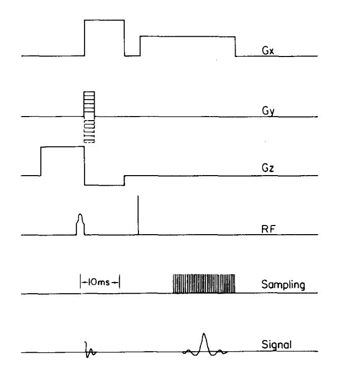
The pulse sequence used to obtain the data for all the images analyzed. The readout gradient is G_x; G_y is the phase encoding gradient, and G_z is the gradient which defines the imaging slice.

The received rf signal is mixed with the transmitted frequency, filtered, and then sampled. The presence of the readout gradient, G_x, during the sampling period couples the x spatial coordinate directly with frequency. The Fourier transform of the sampled signal yields a modulated “projection” of the object centered at Δf = 0, where Δf is the frequency offset from the resonance frequency. A second Fourier transform of a set of projections, performed in the phase encoding direction, yields the final two-dimensional image. If each projection has 256 points and there are 256 projections, a 256 × 256 image results, with the horizontal (x) coordinate in Hz and the vertical (y) coordinate in m/T. This is the 2DFT reconstruction algorithm.⁵

In order to reduce the image acquisition time, it is common practice to reconstruct an image from 128 projections by adding 128 zeros to the data in the G_y direction and then applying a 256-point Fourier transform. This technique approximates sinc interpolation in image space.^5,6 Henceforth, images reconstructed using 128 projections will be called interpolated images and those reconstructed from 256 projections will be called noninterpolated.

For each projection the usual procedure is to sample the signal at 512 points with a sampling interval of 30 μs. These samples are subjected to a 512-point Fourier transform and the resulting 512 points are truncated, removing 128 points from each wing, to produce a 256-point projection. The final image has a 65.1 Hz/pixel dispersion [(30 μs × 512)^-1] in the x direction; thus, the left-and right-hand edges of the image will be at - 8.33 and 8.33 kHz, respectively. The effects of changing the number of samples and the sampling interval will be described later.

Any discrete rf interference or noise in the system would show up as a bright column in the image and be easily identified. Such discrete noise was not detected in these experiments. In fact, most of the noise was thermal noise from the head coil and preamplifier (MITEQ AU-3A-0110, 46-dB gain, 1-dB noise factor). Sampled points of the thermal noise will be statistically independent in the time domain with a Gaussian probability density function. If there is no synchronous noise in the system, each projection is an independent set of these data points. Therefore, the image noise calculated by the 2DFT algorithm will be spatially invariant, provided the sampling is adequate, with a Gaussian probability density function.

The noise power spectrum W (u,v) for a stationary ergodic process is defined as⁷

$$W(u,v)=\langle \underset{X,Y\to \infty }{\lim }(1∕2X)(1∕2Y)\times {\mid {\int }_{-X}^X{\int }_{-Y}^Y\Delta D(x,y)\exp [-2\pi i(ux+vy)dxdy]\mid }^2\rangle ,$$ (1)

where 〈〉 represents an ensemble average and

$$\Delta D(x,y)=I_{\text{mean}}-I(x,y),$$

I (x,y) being the image. The stationary condition implies that the noise is spatially invariant; the ergodic condition implies that one realization of the “process” (i.e., image) will have the same statistical characteristics as any other realization. From the discussion given above on the source of the noise, one can assume that these properties hold for the images analyzed.

A brief description of the NPS may assist those unfamiliar with it. The function ΔD (x,y) has a mean of zero and in our case represents the noise in the image. The Fourier components of this function are calculated and the square of the magnitude of each is normalized by the area over which the transform was calculated. This process is repeated many times and the square of the magnitude at each point in the frequency space is averaged yielding a function W (u,v) which estimates the power per unit area at this point.

In order to facilitate the acquisition of the ensemble average, 256 × 256 pixel images were partitioned into four 128 × 128 quadrants, and the NPS calculated for these smaller fields. The resulting spectrum was a half scale version of that which would have been obtained had 256 × 256 noise fields been used, that is, the range of spatial frequencies available from a 128 × 128 field is - 64 to 63 cycles/field whereas in a 256 × 256 image one can have frequencies from - 128 to 127 cycles/field. The essential “shape” of the power spectrum is unaltered by reducing the size of the field by this amount.

The images analyzed were obtained using phase-sensitive reconstruction; hence, I (x,y) were positive and negative integers. In the NPS calculation I (x,y) is used as the real part of the complex function used in the fast Fourier transform, the imaginary part being set to zero. This implies that the two-dimensional Fourier transform of the data is Hermitian. Thus, only one-half of the resulting complex numbers need be stored, and the final two-dimensional power spectrum is symmetric about the origin.

III. RESULTS AND DISCUSSION

A. Noise power spectra

Figure 2 shows histograms of pixel values calculated from interpolated images of air, reconstructed from data that had 2, 4, and 8 sequences averaged into each projection. Gaussian distributions fit these histograms well. The value of σ for the widest Gaussian fit shown was determined by an RMSD measurement from the image that had two sequences per projection. The other two Gaussian distributions were calculated from the first by reducing σ by a factor of $\sqrt{2}$ for each twofold increase in the number of sequences averaged.

Fig. 2.

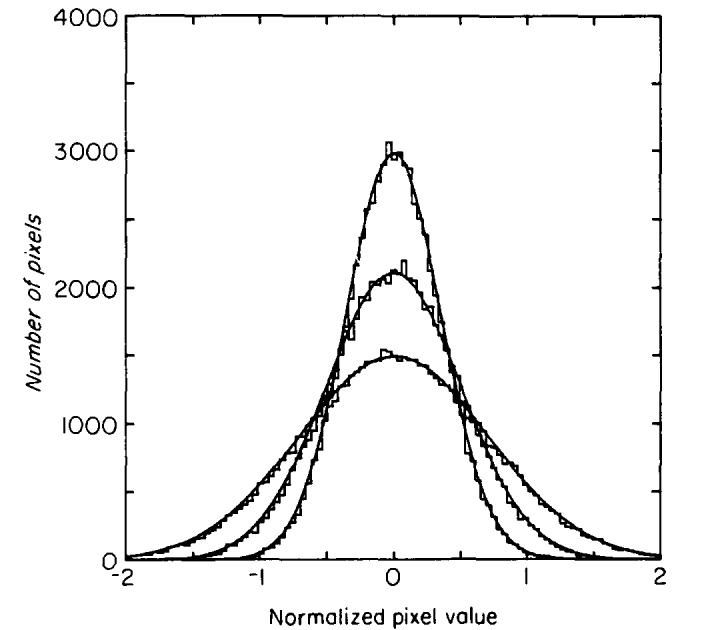
Histograms of pixel values found in interpolated images of air that had 2, 4, and 8 sequences averaged are fitted with Gaussian distributions (solid curves). The widest Gaussian fit was derived from a standard deviation measurement of the 2-sequence image and this width was arbitrarily set to unity. The other two fits were assigned widths of $1∕\sqrt{2}$ and 1/2 showing that the RMSD is proportional to $1∕\sqrt{N}$, where N is the number of sequences averaged.

These images showed no detectable structure; however, a quantitative analysis was done to show the noise was stationary. The histograms of 16 independent subfields of the image were compared with a standard χ² test against the Gaussian distribution derived from the whole field and the noise was found to be spatially invariant. As the number of averages was increased beyond 8, some structure was detected, but the fluctuations remained uncorrelated. In clinical images the number of averages is usually well below 8.

Figure 3 shows the two-dimensional noise power spectrum from 40 independent 128×128 subfields of noninterpolated images. For clarity in the plots, the 128×128 NPS was smoothed to 32×64. This smoothing process obscures the dc component, W(0,0), which had a value of zero. The spectrum shows the anticipated flat structure. Because the amplitude of the NPS is dependent on the gain of the system, the absolute height of each component has little significance. Only comparisons of the magnitude of components within a spectrum are meaningful. The average height of the power spectrum in Fig. 3 was set at unity and all subsequent power spectra acquired with the same system gain, were normalized to this value.

Fig. 3.

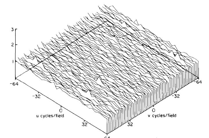
The two-dimensional noise power spectrum W(u,v) obtained from 40 128×128 subfields of a 256×256 noninterpolated image, with two sequences averaged into each projection. The spatial frequencies u and v are the variables conjugate to x and y, respectively. The height of this spectrum was used to normalize subsequent spectra.

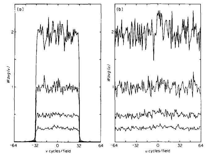
For the sake of clarity the NPS are displayed in subsequent figures as one-dimensional averages W_avg(u) and W_avg(v):

$$\begin{array}{c}\hfill W_{\mathrm{avg}}\left(u\right)=\frac{1}{V_{\max }}\sum _{v=0}^{V_{\max }}W(u,v),\hfill \\ \hfill W_{\mathrm{avg}}\left(v\right)=\frac{1}{U_{\max }}\sum _{u=0}^{U_{\max }}W(u,v),\hfill \end{array}$$ (2)

where U_max and V_max are the maximum nonzero frequency components in the spectrum. For the interpolated images, U_max = 64 cycles/field and V_max = 32 cycles/field; for the noninterpolated images, U_max = V_max = 64 cycles/field. Structures displayed in the one-dimensional spectra are solely dependent on either x or y spatial frequencies. Figure 4 shows that power spectra of both interpolated and noninterpolated images are flat over the available frequency regions. For the algorithm described above, interpolated images have a W_avg(v) that drops to zero rapidly outside ± 32 cycles/field demonstrating that only one-half of the available spatial frequencies are present. This is a graphic illustration of the fact that the spatial resolution in the y direction in a 256×256 interpolated image is only 128 cycles/field, and that no higher frequencies have been introduced by the interpolation algorithm.

Fig. 4.

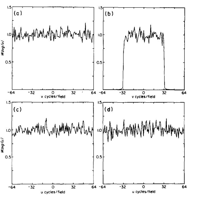
W_avg(v) for (a) noninterpolated and (b) interpolated images. Both spectra are flat over the available frequency range. W_avg(v) for the interpolated image drops to zero rapidly outside ±32 cycles/field because only 128 projections were used in the reconstruction. W_avg(u) for (c) noninterpolated and (d) interpolated images shows the spectra cover all possible frequencies in the x direction.

The similar amplitudes of the two spectra in Fig. 4 can be explained in terms of the RMSD of the original images. The measured RMSD in noninterpolated images is greater than that in interpolated images by a factor of $\sqrt{2}$. This is to be expected since the data in the phase encoding direction for the interpolated image consists of 128 zeros and 128 data points, whereas the data for the noninterpolated image is 256 data points. A pixel value in an image is the sum of these data points modulated by a cosine whose wave number is determined by the displacement of that pixel from y = 0. The same Fourier transform is applied to the data when reconstructing interpolated and noninterpolated images; therefore, the RMSD will increase as the square root of the number of nonzero points in the transform. This is expressed formally by Parseval’s theorem:

$$\sum _{x=1}^{128}\sum _{y=1}^{128}\Delta D{(x,y)}^2=\sum _{u=-64}^{63}\sum _{v=-64}^{63}W(u,v),$$ (3)

where ΔD(x,y) is the deviation from the image mean at pixel (x,y). The variance of the original noise field equals the volume under the power spectrum W(u,v).

The Gaussian distributions shown in Fig. 2 were calculated assuming that the variance of the noise field decreased linearly with the number of sequences averaged into a projection, and the accuracy of the fits confirmed this assumption. Figure 5 shows W_avg for the power spectra of interpolated images which had 1, 2, 4, and 8 sequences averaged. The relative heights of the spectra decrease linearly with the number of sequences averaged, as expected from Parseval’s theorem.

Fig. 5.

(a) W_avg(v) and (b) W_avg(u) for 1, 2, 4, and 8 sequences averaged. The heights of the spectra are inversely proportional to the number of sequences averaged.

In principle the NPS determined from an image of a uniform object should be the same as that measured from images of air, provided the coil remains tuned to 50-Ω, 0° phase. Five interpolated images of a homogeneous flood field phantom filled with a paramagnetic solution were made, and a 128×128 central subfield, which contained only pixels from the image of the phantom, was removed from each. The NPS from these five images matched those of images of air except for a large spike at u = 0, v = ± 1, caused by nonuniform intensity in the phase encoding direction. From this result we conclude that noise in an image at this field strength is independent of signal strength.

B. Spatial filtering

One method of reducing noise in an image is to convolve it with a smoothing function. This technique reduces the variance in the image but blurs sharp edges by an amount related to the shape of the function used in the convolution. This process is equivalent to reducing high spatial frequencies in the image. We have already seen that elimination of high spatial frequencies with a “rectangular filter” (i.e., interpolated versus noninterpolated images) resulted in a lower RMSD for the “filtered” or interpolated image.

In fact, this early truncation of the Fourier series often motivates the application of spatial filters in the y direction. If left unmodified, the truncated series yields edge ringing artifacts at step discontinuities in the image; this is called Gibbs phenomenon.⁸ The truncation of the data also causes large sidelobes in the point spread function, if it does not occur at an integral number of periods of the sinusoids represented by the data.⁹ These phenomena occur in images reconstructed from either 128 or 256 projections, but early truncation exacerbates the problem. In a clinical image the ringing or sidelobes may be mistaken for anatomical structure in complex regions of the image where their artifactual nature is not obvious.

MR imaging is particularly amenable to convolution filtering since the data, obtained in frequency space, can simply be multiplied by a filter function which reduces higher spatial frequencies. The Fourier transform of the filtered data is equivalent to the convolution of the unfiltered image with the Fourier transform of the filter function. This type of filtering does smooth the final image, but the signal-to-noise ratio as a function of frequency is unaffected because both the noise and the signal are reduced by the same factor. With this type of image smoothing there is a compromise between the reduction of noise and artifact, and the loss of spatial resolution.

NPS of unfiltered and filtered images were used to determine the shape of the filter function. Figure 6(a) shows two spectra from images of air filtered in the y direction compared with a spectrum of an unfiltered image. Because a common data set is used, the shape of the square of each filter can be calculated; Fig. 6(b) shows the two filters in frequency space derived from Fig. 6(a). The filters applied to interpolated images were derived similarly and are of a form identical to those shown in Fig. 6 except that their width is reduced twofold to cover the reduced frequency range of the data. No degree of filtration with this function could be found which reduced the edge ringing and sidelobes significantly without an unacceptable loss in spatial resolution. Other methods have been developed to cope with this problem.¹⁰

Fig. 6.

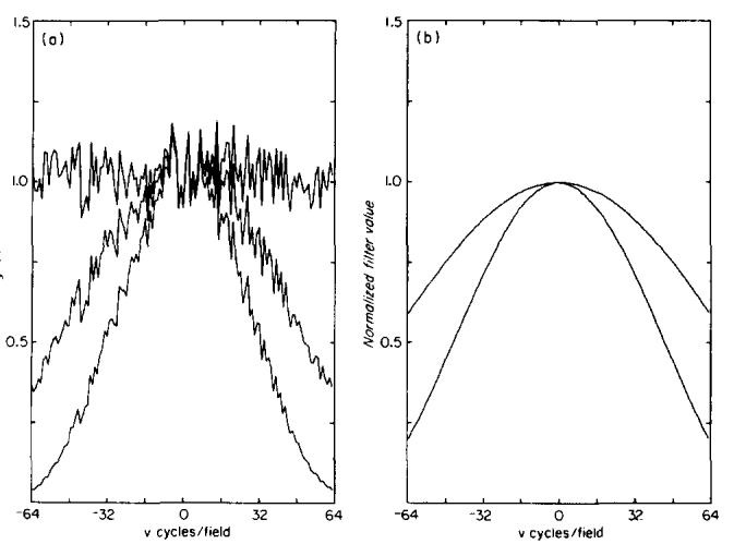
Effect of spatial filtering in the y direction. (a) W_avg(v) for an unfiltered noninterpolated image (top line) is compared with W_avg(v) of two images reconstructed from the same data with increasing filtration. By dividing the filtered results by the unfiltered data, the magnitude squared of the filter frequency response is obtained and the resulting filters are shown in (b).

C. Temporal filtering

The bandwidth of the sampled data is controlled with an electronic low-pass temporal filter applied after mixing. Because each projection is the frequency spectrum of this signal, temporal filtration reduces both signal and noise as one moves away from Δf = 0, possibly decreasing the signal uniformity across the image. The temporal filters must be chosen in appropriate relation to the sampling interval in order to avoid this roll-off as well as aliasing artifacts described below.

A projection is a discrete Fourier transform of a finite number of data points, and is, therefore, periodic with period X = 1/Δt, where Δt is the sampling interval. The frequency X/2 is referred to as the Nyquist frequency. An appropriate temporal filter must substantially attenuate frequencies greater than X/2 in order to reduce overlapping repetitions of the transform, a phenomenon called aliasing. If the sampling interval is too large or the filter passband too wide, the signal over the width of the image will include contributions from the repetitions centered at ±X, ±2X, ±3X,... .

The nature of this phenomenon in MR imaging is illustrated in Fig. 7. The frequency response of a low-pass filter is shown, which has its - 3 dB point or “corner frequency” at 14 kHz. The filter is repeated with period 16.7 kHz because the sampling interval in this example is Δt = 60 μs. Only the first two repetitions are shown in Fig. 7. The solid top line spans the width of the image and shows the resulting normalized RMSD calculated at each value of Δf. Because the noise from the repeated spectra is independent, it is added in quadrature. Thus at Δf = v in Fig. 7, C² = 1 + A² + B² ( + higher order terms).

Fig. 7.

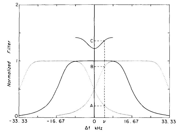
The frequency response of a 14-kHz filter used to band limit the received signal is shown as the lower solid line. The first two periods of the frequency response shown as dotted lines are centered at the frequencies ± 16.7 kHz (Nyquist = 8.33 kHz). The top solid line shows the RMSD calculated across the width of the image including aliasing of noise from these two repeated transforms. Independent noise is added in quadrature; therefore, C² = 1 + A² + B².

In order to investigate this relationship between RMSD and sampling protocol, images of air were reconstructed from data collected with sampling intervals of 15, 30, and 60 μs and filters which had corner frequencies of 7, 14, 29, and 50 kHz. The total sampling time in each case was held at 15 360 μs by varying the number of points collected (1024, 512, and 256 points). For each of the 12 images the RMSD in each column was calculated. Because the data was symmetric about zero the RMSD values for negative frequencies were reflected about the origin and averaged with those for positive frequencies. Four adjacent columns were averaged and plots of RMSD versus frequency from the center to the edge of the image are shown in Fig. 8.

Fig. 8.

RMSD vs frequency from the center to the edge of the image for various sampling protocols and temporal filters. The solid lines are predicted RMSD values; the measured points are □ 7-kHz filter, * 14-kHz filter, ○ 29-kHz filter, × 50-kHz filter. The different sampling protocols are (a) 1024 points at 15-μs intervals, (b) 512 points at 30-μs intervals, and (c) 256 points at 60-μs intervals. All of these yield an image width of 256 pixels with 65.1 Hz/pixel. As the sampling rate is decreased, the amount of aliased noise increases.

Theoretical calculations of RMSD versus frequency for the same sampling protocols were done using the frequency response of the four filters and an estimate of the frequency response of the coil. The RMSD values measured from all images were normalized to the average RMSD found between 0.5 and 3.0 kHz in the image reconstructed from data sampled at 15 μs with a 14-kHz filter. These points should have had no contribution from aliasing, and the filter was flat over this frequency range. The Δf = 0 point was avoided in this normalization because there is often a spurious component at this frequency.

If the data is 1024 points sampled at 15-μs intervals, the period of the frequency response is 66.7 kHz. Equivalently, the Nyquist frequency is 33.3 kHz, which is well away from the image edge at 8.33 kHz. One expects no aliasing to occur for data acquired with the 7-, 14-, and 29-kHz filters in this case. Figure 8(a) shows a plot of RMSD versus frequency measured from the 1024×15 μs images, and the theoretical curves calculated from the filters. With the 7-kHz filter, shown as the lower solid curve, the noise decreases as the image edge is approached.

When 512 samples are acquired at 30-μs intervals the Nyquist frequency decreases to 16.7 kHz. Aliasing now increases the noise uniformly over the image in the case of the 50-kHz filter, as shown by the top line in Fig. 8(b). For the image reconstructed from data obtained with the 29-kHz filter, aliasing produces a nonuniform noise distribution; the RMSD increases as the image edge is approached, as shown by the middle line of Fig. 8(b). No aliasing is predicted or observed for the 14-kHz image, and thus there is a uniform distribution of white noise over the image.

Figure 8(c) shows the results from images reconstructed from 256 data points sampled at 60-μs intervals. The Nyquist frequency in this case is 8.33 kHz, which causes aliasing of noise for all images. The measured data points for the 29- and 50-kHz filters are somewhat lower than the theoretical curves when the Nyquist frequency is well within the passband of the filters. This implies that the value of the response of the system at high frequencies relative to that at low frequencies is smaller than expected. Accurate measurements of the filters confirmed the calculations of their frequency response. The cause of the reduction of high-frequency noise is likely a slow roll-off in the high-frequency response of the system, the exact origin of which has not been determined. In spite of this discrepancy, calculated and measured RMSD values shown in Fig. 8 agree within 10%.

For a uniform distribution of signal across the image the filter corner frequency must extend beyond the image edge. In order to limit the aliased noise to 10% of the total noise level as reflected by the RMSD, the filter must drop to approximately - 7 dB before the frequency Δf = (2× Nyquist) - (image bandwidth/2). In the case of images where the edges are ± 8.33 kHz (16.7-kHz bandwidth), the 14-kHz filter coupled with a sampling of 512 points at an interval of 30 μs gives the desired result [Fig. 8(b)].

IV. CONCLUSIONS

The noise measured in unfiltered images was found to be normally distributed, spatially invariant, and white, in agreement with theoretical expectations. This suggests that the imager performs ideally in terms of noise propagation. The spatial filters used to smooth image noise and artifacts were shown from ratios of the calculated noise power spectra to be simple low-pass filters with approximately Gaussian frequency response. These filters were inadequate in suppressing truncation artifacts and other methods are recommended.¹⁰

Temporal filtering is applied to the spin-echo signal to minimize image noise. A temporal filter with too narrow a frequency response diminishes the signal at the edges of the image in the x direction. Too broad a frequency response in the temporal filter introduces additional noise through aliasing. A uniform signal with no additional aliased noise is achieved with over sampling by a factor of 2 in the x direction coupled with a temporal filter that is flat over the image bandwidth and falls to below - 7 dB before the frequency Δf = (2×Nyquist) - (image bandwidth/2).

The noise power spectrum of a homogeneous phantom was found to have the same amplitude and structure as background noise; thus, background noise is a good indicator of the noise throughout the image. For the system we have measured, no improvement in the image noise can be anticipated from filtering without reducing the source of the noise.

References

- 1.Proc. IEEE. 1982;70(9) [Google Scholar]
- 2.Hoult DI, Lauterbur PC. J. Magn. Reson. 1979;34:425. [Google Scholar]
- 3.Burgess AE, Wagner RF, Jennings RJ. IEEE Society “Proceedings International Workshop on Physics and Engineering in Medical Imaging”; 1982; pp. 99–105. (IEEE Catalogue No. 82CH1751-7) [Google Scholar]
- 4.Wagner RF, Brown DG, Burgess AE, Hanson KM. Magn. Reson. Med. 1984;1:76. doi: 10.1002/mrm.1910010109. [DOI] [PubMed] [Google Scholar]
- 5.Kumar A, Welti D, Ernst R. J. Magn. Reson. 1975;18:69. doi: 10.1016/j.jmr.2011.09.019. [DOI] [PubMed] [Google Scholar]
- 6.Bartholdi E, Ernst R. J. Magn. Reson. 1973;11:9. [Google Scholar]
- 7.Dainty JC, Shaw R. Image Science. Academic; New York: 1974. p. 222. [Google Scholar]
- 8.Papoulis A. The Fourier Integral and Its Applications. McGraw-Hill; New York: 1962. p. 30. [Google Scholar]
- 9.Brigham EO. The Fast Fourier Transform. Prentice-Hall; Englewood Cliffs: 1974. pp. 91–109.pp. 140–146. [Google Scholar]
- 10.Wood M, Henkelman RM. Magn. Reson. Med. 1985;2:6. doi: 10.1002/mrm.1910020602. [DOI] [PubMed] [Google Scholar]