

Abstract
When ionizing radiation is used in cancer therapy it can induce second cancers in nearby organs. Mainly due to longer patient survival times, these second cancers have become of increasing concern. Estimating the risk of solid second cancers involves modeling: because of long latency times, available data is usually for older, obsolescent treatment regimens. Moreover, modeling second cancers gives unique insights into human carcinogenesis, since the therapy involves administering well characterized doses of a well studied carcinogen, followed by long-term monitoring.
In addition to putative radiation initiation that produces pre-malignant cells, inactivation (i.e. cell killing), and subsequent cell repopulation by proliferation can be important at the doses relevant to second cancer situations. A recent initiation/inactivation/proliferation (IIP) model characterized quantitatively the observed occurrence of second breast and lung cancers, using a deterministic cell population dynamics approach. To analyze if radiation-initiated pre-malignant clones become extinct before full repopulation can occur, we here give a stochastic version of this IIP model. Combining Monte Carlo simulations with standard solutions for time-inhomogeneous birth-death equations, we show that repeated cycles of inactivation and repopulation, as occur during fractionated radiation therapy, can lead to distributions of pre-malignant cells per patient with variance ≫ mean, even when pre-malignant clones are Poisson-distributed. Thus fewer patients would be affected, but with a higher probability, than a deterministic model, tracking average pre-malignant cell numbers, would predict. Our results are applied to data on breast cancers after radiotherapy for Hodgkin disease. The stochastic IIP analysis, unlike the deterministic one, indicates: a) initiated, pre-malignant cells can have a growth advantage during repopulation, not just during the longer tumor latency period that follows; b) weekend treatment gaps during radiotherapy, apart from decreasing the probability of eradicating the primary cancer, substantially increase the risk of later second cancers.
Keywords: ionizing radiation, mathematical modeling, computational radiobiology, carcinogenesis, stem cell repopulation
Introduction
Ionizing radiation is a carcinogen as well as an agent for killing cells. When radiotherapy is used to eradicate a tumor, the radiation can cause second cancers, e.g. in organs adjacent to the tumor [reviewed in (Curtis et al., 2006; Hall, 2006; Little, 2001; Ron, 2003)]. With screening resulting in patients being treated at younger ages, and withincreasing patient survival times, second cancers are becoming of increasing concern (Travis et al., 2006). The long time lag between radiotherapy and second cancer incidence means that few direct data, or none, are available on second cancers induced by recently introduced treatment modalities, so that model-based predictions are important.
Models of Radiation Carcinogenesis Used in Applied Risk Estimation
Radiation carcinogenesis, in this second cancer situation and in general, is a complex process. But it is important to have a well defined, consensus, quantitative method to get some estimate of the cancer risk. In many practical applications [e.g. (Bennett et al., 2004; Brenner et al., 2003; Land et al., 2003; Preston et al., 2003; Walsh et al., 2004)] it is assumed as an approximation that the year-specific excess relative radiation risk (ERR) of cancer incidence for a specified organ, defined conceptually in terms of the ratio of the relevant hazard functions, has a product form, i.e.
| (1) |
Here A depends on radiation parameters (e.g. radiation type, dose, and dose-timing), while B depends on time since irradiation and on demographic factors (e.g. age at irradiation, gender, ethnicity) but not on the dose or dose timing. Implicit in Eq. (1) is the idea that there are really two time scales involved: A is determined by processes that occur during a comparatively short irradiation time; B by processes that occur subsequently, during a comparatively long latency period before tumors are incident clinically. An important implication of Eq. (1) is that various predicted ERR dose-response curves all have the same shape (i.e. differ only in vertical scale): one curve for dose-dependence of damage comparatively soon after irradiation; others for dose-dependence of ERR during each particular subsequent year.
“Biologically-based” radiation carcinogenesis models [e.g. (Hanin et al., 2006; Heidenreich et al., 2004; Moolgavkar and Luebeck, 2003; Pierce, 2003; Sachs et al., 2005; Yakovlev and Polig, 1996)] analyze the longer-time latency period in more detail. Such biologically based models usually do not assume or imply the product form, Eq. (1), for the ERR; they often do have this product form as an approximation. They can also be used when radiation is so protracted it involves times comparable to the latency time, in which case the two time scale assumption underlying Eq. (1) does not apply. However, such biologically based models are as yet less thoroughly explored and less accepted than the models actually used in current applied risk estimation, which do assume Eq. (1), as we consequently also will in the present paper.
For a single dose of magnitude d administered acutely (i.e. rapidly compared with endogenous cellular times such as DNA repair times or cell cycle times) the dose-dependent factor A in Eq. (1) has in the past usually been taken to have the following “linear-quadratic-exponential” form [reviewed in (Bennett et al., 2004; Dasu et al., 2005; Radivoyevitch et al., 2001)]:
| (2) |
Here a, b,α and β are non-negative parameters. This form is usually rationalized, in terms of cell initiation and inactivation, as follows:
a) Putatively, the first step in carcinogenesis by ionizing radiation is the “initiation” of target cells to form cells, that are “pre-malignant” in the sense that they may eventually evolve into a clinically detectable cancer. The molecular nature of the initiation event and the biological scenario for subsequent evolution of the initiated cells are left open in almost all applications of Eq. (2), the emphasis being instead on the numerical values of the four parameters and on the resulting dose dependence. For example, Eq. (2) does not specify whether the radiation-produced initiation is a single point mutation, much larger-scale genome damage such as aneuploidy, or some other kind of event.
b) The factor exp(-αd-βd2) is the standard linear-quadratic (LQ) estimate of cell survival – the probability that a cell is not inactivated by the dose (i.e. is still capable of originating a clone). The quadratic term βd2 represents “two-track action” where damage from two different radiation tracks interacts to inactivate the cell; the linear term αd represents one-track inactivation [reviewed in (Guerrero et al., 2002; Jones et al., 2001; Sachs and Brenner, 1998; Sachs et al., 1997)]. In most environmental or occupational risk estimation situations, the relevant doses are so low that exp(-αd-βd2)=1 to good approximation, but for second cancer scenarios such is by no means the case.
c) The factor (ad+bd2) is a standard LQ estimate for the product pN, where N is the number of target cells and p is the probability a target cell is initiated to make a pre-malignant cell. Here p ≪ 1 since N, e.g. the number of stem cells in a normal breast, is believed to be 107 or more (Clarke, 2005; Paguirigan et al., 2006) whereas, in the situations of interest here where stochasticity is important, the number of initiated cells has order of magnitude unity
During the last half century, there have been many vigorous controversies about which kind of situations can be usefully approximated by Eq. (2), and about the values of the four parameters. Current disagreements about the applicability of this equation are especially heated for the initiation term (ad+bd2) in situations where the total doses involved are much lower than those used in radiotherapy, as illustrated by strongly contradictory views of the U.S. and French National Academies of Science (NRC, 2005; Tubiana et al., 2005). However, using, modifying, and/or generalizing Eqs. (1) and (2) is a basic starting point of almost all current applied radiation carcinogenesis risk analyses, and these two equations lead to a useful first approximation to most more sophisticated models. We shall here also start with Eqs. (1) and (2), emphasizing modifications needed in the factor A, particularly at high doses where our approach differs significantly from older approaches, to account for radiotherapy dose-fractionation and for cell proliferation during or shortly after radiotherapy. The stochastic aspects of cellular initiation, inactivation, or proliferation are emphasized. The factor B, whose evaluation typically involves epidemiological data, e.g. data on the Japanese atomic-bomb survivors, will be discussed only briefly.
Fractionated Radiotherapy
Most external beam, fractionated, solid tumor radiotherapy regimens have the following features:
a) Dose-fractions lasting less than 30 minutes are administered daily (omitting weekends). The number K of dose-fractions is typically in the range 20-45.
b) The total prescribed dose D to the tumor is in the range 45-85 Gy (1 Gy = 1 Gray = 1 Joule/kg); nearby regions of the body are unavoidably also irradiated; in some proximal regions the dose is comparable to the prescribed dose.
c) Dose-fractions are usually equal, in which case the dose d for each fraction is d=D/K.
For fractionated radiotherapy under these conditions, the standard extension of Eq. (2), re-derived in Appendix B in order to display explicitly the assumptions involved, is
| (3) |
Eq. (3) is an “initiation/inactivation” equation, with the LQ factor [aD+(bD2/K)] representing initiation and the LQ factor exp[-αD-(βD2/K)] representing inactivation. The factors (1/K) arise basically because two-track action does not occur if the two radiation tracks are separated by more than a few hours (i.e., occur in different dose fractions), repairable damage from the first track being almost wholly repaired before the second track arrives [review: (Sachs et al., 1997)]. Eqs. (1) and (3) have been the main formalism for estimating radiogenic second cancer risks [recent examples include (Bennett et al., 2004; Dasu et al., 2005)].
Weaknesses of the Initiation/Inactivation Equation, Eq. (3)
In Eq. (3), radiation plays a dual role, initiating some normal cells but also inactivating some initiated cells. For realistic values of the parameters, the exponential (inactivation) factor exp[-αD-(βD2/K)] in Eq. (3) is so small at total doses above about 15 Gy that the predicted number of second cancers is negligible –essentially, the prediction is that there is no carcinogenesis because no pre-malignant cells survive. However, recent data indicates that in fact substantial second carcinogenesis can occur at high total doses, such as those used in radiotherapy [reviewed in (Sachs and Brenner, 2005; Schneider and Kaser-Hotz, 2005)]. A likely source of this discrepancy is that Eq. (3), as shown explicitly by its derivation (Appendix B), neglects cell proliferation between dose-fractions and during the recovery period following the last fraction. Wheldon and co-workers [e.g. (Lindsay et al., 2001)] pointed out that, to the contrary, repopulation by cell proliferation, which is a very well known adverse factor for radiotherapeutic eradication of primary tumors [reviewed in (McAneney and O’Rourke, 2007)], almost certainly also influences second cancer induction. Symmetric proliferation of normal and of pre-malignant stem cells is expected to increase carcinogenesis (Fig. 1).
FIG. 1. Influences on carcinogenesis risks: initiation, inactivation, and proliferation.

Radiation carcinogenesis involves radiation initiation that makes normal cells pre-malignant (Panel A). In radiotherapy, because of the high doses used, a significant fraction of the pre-malignant cells initiated by previous fractions in nearby tissue, and of the normal cells at risk for initiation in subsequent dose-fractions, are inactivated by radiation (Panel B). After cell inactivation, repopulation via symmetric proliferation occurs (Panel C). Repopulation tends to increase second cancer risks for two reasons: a) among the proliferating cells are some pre-malignant ones; and b), proliferation replenishes the pool of normal cells at risk for initiation in subsequent fractions.
The classic initiation/inactivation model for second tumors, given by Eqs. (1) and (3), does not take proliferation into account; it predicts very low carcinogenesis risk at sufficiently high doses, due to inactivation. However, initiation/inactivation/proliferation (IIP) models for second tumors take repopulation into account and predict substantial carcinogenesis risks at high doses, due to proliferation counteracting inactivation.
Deterministic and Stochastic Initiation/Inactivation/Proliferation (IIP) Models
To explain epidemiological data on solid second tumors, cellular repopulation by proliferation was added to the initiation/inactivation model given by Eqs. (1) and (3). The resulting initiation/inactivation/proliferation (IIP) model (Sachs and Brenner, 2005) was based on the following equations : a) Eq. (2) to describe initiation in each dose-fraction; b) standard LQ equations to describe inactivation of normal and of radiation-initiated pre-malignant stem cells in each dose-fraction (Appendix B); and c), a system of two nonlinear ordinary differential equations to describe cell repopulation dynamics between dose-fractions or after the last dose-fraction (Appendix B). This model gave results consistent with data on radiation-induced breast or lung cancers following radiotherapy treatment for Hodgkin disease. However, the model neglected stochastic fluctuations of the pre-malignant cell number.
Such fluctuations may play a key role. For a related problem – tumor eradication by fractionated external beam radiotherapy – stochastics have been studied in detail for some time (Tucker et al., 1990). An explicit analytic solution for a relevant time-inhomogeneous birth-death process with additional fractionated cell killing has been found [(Zaider and Minerbo, 2000); (Hanin, 2004) and references there]. Our calculation here differs, mainly because we include initiation, but it is known (Little, 2007; Sachs and Brenner, 2005; Shuryak et al., 2006; Tucker and Taylor, 1996) that in either situation, for fractionated radiation with large total doses, repeated cycles of inactivation and proliferation can lead to statistical distributions of cell numbers where the ratio of variance to mean is much larger than the value 1 that a Poisson distribution would imply [“overdispersion”; compare (Boucher et al., 1998)]. Correspondingly, the zero class probability, interpreted in our setting as the fraction of patients who do not have any radiation-initiated, pre-malignant cells, can be much larger than anticipated from the mean number of radiation-initiated cells per patient. These considerations correspond to a typical eradication scenario: if, just after the last dose-fraction, every cell in every radiation-initiated pre-malignant clone has been inactivated, by radiation or other mechanisms, then subsequent cellular repopulation does not add any radiation risk.
Preview
The present paper concerns carcinogenesis in second cancer scenarios, taking into account stochastic inter-patient fluctuations in pre-malignant cell number for patients who are otherwise identical. We shall first review the deterministic IIP model. Then we describe and apply a stochastic version of the model. In the stochastic model we analyze clones initiated by the radiation during a particular dose-fraction and the distribution of cell numbers for such a clone. A clone can ultimately lead to cancer incidence with some probability, with different clones presumably acting independently since they will typically originate at different random locations in an organ. In principle the way the probability of ultimate cancer incidence depends on the number of cells in a clone would need to be specified. Here we consider a limiting case which is the opposite extreme of the deterministic case – i.e. corresponds to the most pronounced stochastic effects. Specifically we assume that any clone which is present after repopulation has run its full course ultimately gives rise to a second cancer. This limiting case is assumed, explicitly or implicitly, in many biological analyses of “cancer stem cells” [reviewed in (Lynch et al., 2006)]. It is considered because it minimizes the number of adjustable parameters and the actual situation is expected to be intermediate between the situation predicted by the deterministic model and this limiting case stochastic model.
Methods
Deterministic IIP Model
The deterministic IIP equations (Appendix B) deal with time-dependent average numbers, n(t) and m(t), of normal and initiated stem cells respectively, for a specified organ. As will be discussed later, these equations are implied by the equations of the stochastic IIP model, which tracks not just averages but the full distributions, and the deterministic model gives considerable insight into the stochastic one. In the models it is assumed that the excess absolute risk in any one year is much less than unity. Instead of using Eq. (3), for the deterministic model the factor A in Eq. (1) is taken to be proportional to mfinal, the value of radiation-induced pre-malignant cell number m(t) at the “final” time, i.e. the time when the normal cell number n(t) has effectively returned to its setpoint and post irradiation repopulation has effectively run its full course (Fig. 2). By Eq. (1) the dose-dependence of mfinal determines the shape of the predicted ERR dose-response curve. The deterministic IIP model is a special case of a somewhat more general model (Appendix A). To calculate mfinal we previously assumed that, when m is negligible compared to n, repopulation between dose fractions (or during the recovery period following the last dose fraction) is described by the following differential equations (Sachs and Brenner, 2005):
FIG. 2. Deterministic cell repopulation dynamics and the compensation theorem.

Normal, and radiation-initiated pre-malignant, average stem cell numbers, n(t) and m(t) respectively, rescaled for convenience, are shown as a function of time since the start of radiotherapy. Calculations were done using the deterministic IIP model (Appendix B) with the following parameters: fraction number K =20 acute dose-fractions, starting on a Monday and continuing daily except for Saturdays and Sundays; dose per fraction to a nearby organ d=1 Gy; initiation constants a=0.75 Gy-1, b=0; relative fitness of pre-malignant cells r=1; inactivation constants α= 0.3 Gy-1 and β = 0.025 Gy-2; and repopulation maximum-rate constant λ=0.3 day-1. In this deterministic IIP model the numerical value of a is not needed for estimates of ERR (due to renormalizing by referring to atom bomb survivor data, as discussed in the text), but the value of a does matter to the numerical value of m, and we here chose an illustrative value of a. A numerical estimate of the setpoint number N is not needed because the only way n(t) and N appear in the calculations is via the ratio ν = n/N (Appendix B); presumably N≈107 or more in most cases.
It is seen that according to the model some normal stem cells (n, red curve) are inactivated in each dose-fraction; then symmetric proliferation causes some repopulation between fractions, especially on weekends. After radiotherapy stops, n grows back to the setpoint number N. Predictions for the average pre-malignant cell number (m, black curve) are the following: at first m grows due to initiation and symmetric proliferation; as m grows, inactivation increases proportionately and starts to overpower initiation; at that point the only effect that tends to increase m is symmetric proliferation, especially during a weekend; finally, after treatment stops, m resumes growth.
It is seen that by t = 60 days, repopulation has essentially run its full course. In the text we refer to this time as the “final” time and identify m(60 days) with mfinal. In the formal calculations, the difference between m(60) and m(∞) is negligible. However, in this context “final” refers to the comparatively short, radiotherapy time scale only. For the long (multiyear) time scale latency period during which a pre-malignant clone progresses into a clinical cancer, 60 days would actually count as the initial time instead. We do not model such progression mechanistically here, circumventing such modeling by the use of the factor B in Eq. (1), and will thus use the word “final” as specified above.
The blue curve, for pre-malignant cell number m*, shows a hypothetical situation in which only initiation occurs at each dose fraction, with α=0=β that no inactivation occurs (and thus there is so also no subsequent repopulation). Then m* simply grows in 20 equal steps. It is seen that ultimately m and m* reach exactly the same value mfinal = Kad, illustrating in this special case the result that, whenever r=1, repopulation exactly compensates for inactivation (Appendix A, Theorem 1). For r≠1, however, the interplay between initiation, inactivation, and proliferation means computer algorithms are needed to evaluate mfinal even in the deterministic IIP model.
| (4) |
| (5) |
In Eqs. (4) and (5) the following hold: λ is a constant representing the maximum per-cell proliferation rate; F(n) ≡ λ [1- (n/N)] is a standard logistic factor with the constant N representing a set point number of normal stem cells at risk; r is a constant, the “relative fitness”, describing any growth advantage or disadvantage pre-malignant cells may have compared to their normal counterparts; and in our applications m≪n at all times. The equations incorporate the idea that, with m≪n, the “density” effects described by F are effectively determined by the size of n(t).
Because they take advantage of n≫m, our equations are quasi-linear in the following sense: the non-linear equations for normal cell number n(t) do not involve m(t), and can be solved first. Then the equations for m(t) are linear in m(t), with coefficients that depend on n(t).
Stochastic Initiation/Inactivation/Proliferation (IIP) Model
A corresponding stochastic model is given in Appendix C. For computational speed, normal stem cells are described only via their average number -- the equations for n(t) are taken over without change from the deterministic IIP model. The number of initiated cells, however, is described by an integer-valued random function m(t), using the following assumptions:
a) Inactivation by one dose-fraction of a preexisting pre-malignant cell is described by a Bernoulli distribution with parameter exp(-αd-βd2).
b) During a dose-fraction, some cells are newly initiated and survive the fraction; these have a Poisson distribution with parameter (ad+bd2)(n-/N) exp(-αd-βd2), where n- is the number of normal cells present just before the dose-fraction; here the factor (1/N), which could have been absorbed in the adjustable parameters a and b, is inserted for later convenience.
c) Between dose-fractions, and after the last fraction, initiated cells undergo a time-inhomogeneous Feller-Arley birth-death process whose parameters depend on the density of normal cells; specifically, the birth rate minus the death rate at any instant is taken to be the deterministic proliferation rate, rλ{1 − [n(t)/N]}.
d) Standard assumptions hold on independence of the random variables involved.
e) ERRs are calculated by assuming that the factor A is proportional to the average number of patients who have at least one radiation-produced pre-malignant cell at the “final” time defined in the caption to Fig. 2. Thus it is the presence or absence of pre-malignant cells at the “final” time, not their average number as in the deterministic IIP model, that is assumed to determine radiogenic excess risk.
As in the deterministic IIP model (Sachs and Brenner, 2005), the ERR is calculated for comparatively low doses using atomic bomb survivor data and standard methods for “translating” the results from a Japanese to a Western cohort (Land et al., 2003). Because B is dose-independent and all our final estimates involve the product AB, not either factor separately, the following steps then suffice to give ERRs at higher doses. Using a mixture of Monte Carlo and analytic methods, we follow a clone of cells whose most recent common ancestor is a cell initiated in the kth fraction (k=0, 1, …K; here k=0 refers to any pre-malignant cells that may have been present before treatment starts). Using assumptions a) and c) above, and iterating over the remaining dose-fractions, we calculate the probability distribution for the number of cells in such a clone at the final time. In particular this distribution gives the probability that a clone will become extinct by the final time, and gives the mean number of cells per clone at the final time. From these two quantities, we calculate, by conditioning on fraction number k as discussed in detail in Appendix C, the three quantities of main interest: the mean number of pre-malignant clones per patient at the final time; the mean number of pre-malignant cells per patient at the final time (due to quasi-linearity this number turns out to be the same as the number predicted by a deterministic IIP model with the same parameters); and the “zero-class” probability, i.e. the fraction of patients who have no radiation-initiated clones in the relevant organ at the final time. This procedure gives A at any dose, and calculating AB at low doses from the atomic bomb survivor data gives B, completing the estimate.
Data Sets and Analysis
We analyzed two data sets, chosen mainly because dosimetry information was more detailed than in other studies, in the literature on breast cancer incidence in women who had received radiotherapy for Hodgkin disease. One (Travis et al., 2003) was a matched case-control study within a cohort of 3817 female 1-year survivors of Hodgkin disease diagnosed at age 30 years or younger, between January 1, 1965, and December 31, 1994, and within 6 population-based cancer registries. Record-linkage techniques were used to identify women who developed a second primary breast cancer. For each documented case, at least 2 controls were selected by stratified random sampling from the cohort. Matching factors were registry, calendar year of Hodgkin disease diagnosis, age at Hodgkin disease diagnosis, and length of survival without a second cancer at least as long as the interval between the diagnoses of Hodgkin disease and breast cancer in the case. Using dose reconstruction techniques, doses were estimated both to the specific location in the breast where cancer developed for each case, and to the corresponding anatomical site in matched controls. Conditional regression analysis was conducted to obtain maximum likelihood estimates of the relative risk of breast cancer associated with specific treatments by comparing the exposure histories of the cases with those of individually matched controls.
The other data set (van Leeuwen et al., 2003) was a nested case–control study for a cohort of 770 female patients who had been diagnosed with Hodgkin disease before age 41 between 1965 and 1988. Detailed treatment information and data on reproductive factors were collected for 48 case patients who developed histologically confirmed breast cancer 5 or more years after diagnosis of Hodgkin disease and 175 matched control subjects. The radiation dose was estimated to the area of the breast where the case patient’s tumor had developed and to a comparable location in matched control subjects. Relative risks of breast cancer were calculated by conditional logistic regression. Follow-up as to the recent medical status of the patients was estimated to be complete for 91% of the cohort members. 650 of those patients survived 5 or more years. Results of the stochastic IIP model were fitted to both data sets simultaneously. For the present, proof of principle, calculations we held all relevant parameters except r, α and β fixed at the deterministic values; for selected values of α and β, r was determined using a least squares algorithm weighted with inverse estimated variance.
Results
Rescaling
The IIP equations (Appendices B and C) describe inactivation and initiation by an acute dose, followed by partial repopulation, followed by another acute dose, followed by more repopulation, etc. (Figs. 1 and 2). In all essential calculations, normal cell number n(t) and setpoint number N always appear only in the ratio defining the rescaled normal cell number, ν = n/N, never separately or in any other combination.
Superposition Principles for Initiated Cell Numbers
Due to quasi-linearity as defined below Eq. (5), typical superposition results hold for the average pre-malignant cell number m(t) and the corresponding random variable m(t). For example, the final average number of pre-malignant cells is a sum of two terms. One term is due to cells which were present before treatment started and were then subject to all the cycles of inactivation and repopulation; the other term is due to cells that were initiated by one of the dose-fractions.
Theorem on Proliferation Compensating for Inactivation
In the deterministic IIP model consider the case where r =1, so that normal and pre-malignant cells have identical repopulation dynamics; then the predicted dose dependence of second cancer ERR is the same as if neither inactivation nor proliferation occurred at all. Specifically theorem 1 in Appendix A implies that for the special case r =1
| (6) |
Here: mfinal is the average number of radiation-induced pre-malignant cells at the “final” time (Fig. 2); and (ad+bd2)/N is the probability of initiating one normal cell in the kth dose-fraction to make one pre-malignant cell just after the fraction, without regard for the fact that actually some of the newly initiated cells are also inactivated by the same dose or that some of the target cells may have been inactivated by previous dose-fractions -- such inactivation is cancelled out by subsequent proliferation. If b=0, then mfinal is just proportional to total dose D=Kd. Fig. 2 shows a special case illustrating the theorem. For r≠1 however, no simple formula such as Eq. (6) for mfinal is known and presumably none exists; numerical methods are used to obtain mfinal.
Stochastic vs. Deterministic Results
Fig. 3 shows some representative results for the stochastic IIP model, compared to the deterministic IIP model having the same parameters and to two other models that are often used. The models differ in the way that they extrapolate lower dose estimates, based on Japanese atomic bomb survivor data, to the higher doses also relevant in second cancer scenarios. A key point in the Fig. 3 is that, even assuming pre-initiated, pre-malignant stem cells have a growth advantage over normal stem cells during repopulation (i.e. r >1), the ERR curve for the stochastic IIP model here has monotonically decreasing slope. On the other hand, when r > 1, the predicted curves of the deterministic IIP model always have a slope that increases as dose increases. Increasing slope contradicts epidemiological estimates, so that in the deterministic model r ≤ 1 has previously been assumed (Sachs and Brenner, 2005).
FIG. 3. Different models of ERR.
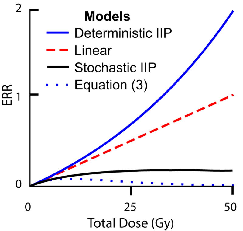
Four models of ERR are shown. We show the case where all four agree at low doses, i.e. the slope of all four curves are the same at the origin, because all four models use renormalization (based on atomic bomb survivor data) at low doses. When extrapolated to higher doses, the models give different results. The parameters used are: K=25 acute dose-fractions, starting on a Monday and continuing daily except for Saturdays and Sundays; initiation factors a= 0.004 per Gy, b=0; relative fitness r=1.2; inactivation constants α= 0.1 Gy-1 and β= 0; rate constant λ=0.3 day-1; and ratio of death rate to birth rate c=0.2. Only the stochastic initiation/inactivation/proliferation (IIP) model requires all of these parameters; for example Eq. (3) contains only a, b,α, and β. To show qualitative trends, the figure here compares different models holding common parameters fixed. If any one of the models is used in fitting data, some parameters are adjusted to fit the situation, and the adjustments would usually lead to different parameters for different models fitting the same data (see Fig. 5 for an example).
Reading from top to bottom, the deterministic IIP model (blue curve), using mean pre-malignant cell number, shows an increase in ERR at high doses. This is attributed to a growth advantage that the pre-malignant cells have (r>1), which comes into play especially at high doses. The linear model (dashed red line) just extrapolates the low dose slope to high doses. According to the compensation theorem proved in Appendix A, a deterministic IIP model with r=1 (instead of r=1.2) and any values for its other parameters would give this linear curve. The stochastic IIP model (black solid curve), based on presence or absence of pre-malignant cells, has slope decreasing as dose increases, despite the growth advantage. Finally, the older model (dotted blue curve), given by Eq. (3), predicts almost no ERR at high doses, putatively due to inactivation of pre-malignant cells wholly uncompensated by proliferation (Fig. 1).
Fig. 4 shows a reason for the difference between the deterministic and stochastic estimates. Calculations using the stochastic IIP model predict that as the dose increases, what increases is not so much the number of patients having surviving clones of initiated, pre-malignant cells but the number of pre-malignant cells per clone. This leads to situations where only a few patients have any radiation-induced pre-malignant cells, but those patients have many pre-malignant cells, corresponding to “overdispersion” in pre-malignant cell number, i.e. a variance much larger than the mean.
FIG. 4. Predicted properties of clones.
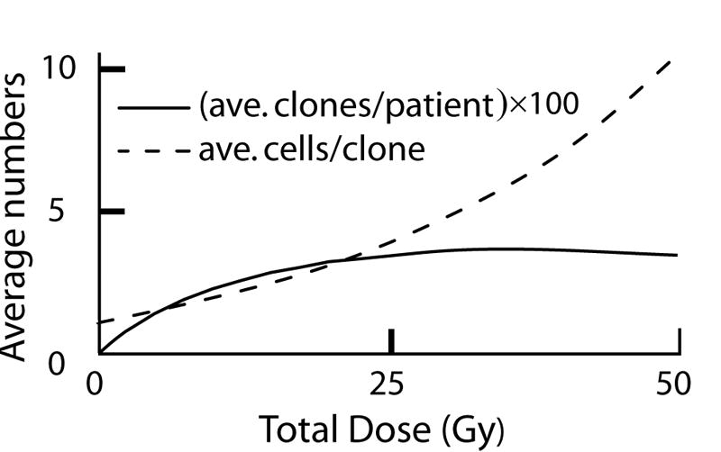
The figure shows predictions of the stochastic IIP model with the same parameters as those used for Fig. 3. The average number of radiation-initiated pre-malignant clones per patient is shown (rescaled for convenience in graphing, the actual maximum is ~0.04 pre-malignant clones per patient). It is seen that at high doses the predicted number of pre-malignant clones per patient does not increase, clones made in earlier dose-fractions being eradicated by later dose-fractions. However, the average number of radiation-initiated, pre-malignant cells per patient continues to increase, as the average number of cells in those clones that do happen to survive increases due to repopulation (i.e. to proliferation following inactivation).
Modeling Second Cancers in Hodgkin Disease Patients
We previously considered data on patients treated with radiotherapy for Hodgkin disease, some of whom subsequently developed second breast cancer (Sachs and Brenner, 2005). Fig. 5 shows that, with selected parameter choices, the stochastic IIP model can fit this data as well as the previously used deterministic IIP model. Because the stochastic model has additional adjustable parameters, the fact that it can be forced to fit the data approximately was not surprising. However, it is of interest to note that only for small values of the inactivation constants α and β is an acceptable fit of the stochastic model available. For values of α and/or β markedly larger than those shown in the figure caption, high doses merely lead to a few pre-malignant clones having a very large number of cells per clone. For still lower values of the radiation sensitivity to inactivation, less extreme values of the other parameters can be used in the stochastic IIP model; for example a roughly comparable fit (not shown in Fig. 5) is obtained with α= 0.04 Gy-1, β=0, λ =0.3 day-1 (i.e. less rapid repopulation), r=1.5, a= 0.004 Gy-1, b=0, c=0.1.
FIG. 5. Comparing different models with data on second breast cancers.

The data sets used, set 1 (Travis et al., 2003) and set 2 (van Leeuwen et al., 2003), are described in the Methods section. The figure shows predictions, all of which use K=25 acute dose-fractions, starting on a Monday and continuing daily except for Saturdays and Sundays. For the deterministic IIP model (dotted blue curve), the relative fitness for initiated, and thus pre-malignant, cells is r=0.825; the initiation constants are a= 0.004 Gy-1 and b=0; the linear inactivation constant is α= 0.18 Gy-1; the quadratic inactivation constant is β=0; and the proliferation rate constant is λ=0.4 day-1. By the theorem in Appendix A, the linear model (dashed brown curve) would result from r=1 in the deterministic IIP model with the given initial slope. For the stochastic IIP model (solid black curve) values used are r=2 (i.e. pre-malignant cells have a strong growth advantage), initiation constants a= 0.004 Gy-1 and b=0 as before, α= 0.075 Gy-1 and β=0 (i.e. low radiation sensitivity), λ=1.5 day-1 (i.e. rapid repopulation), and a ratio c=0.2 of death rate parameter to birth rate parameter for pre-malignant cells. For all three curves, the slope at the origin is determined using data on atomic bomb survivors (see text)
Note that the stochastic IIP model curve in Fig. 5 incorporates a growth advantage for the pre-malignant cells during the repopulation period (i.e. r >1). Unless such a growth advantage is assumed, the stochastic model gives predicted high-dose values too small to match the pattern of the data.
Discussion
Summary
We have reviewed the deterministic IIP model and presented a stochastic version. The most important new conclusion from the stochastic IIP model is that a growth advantage for initiated and thus pre-malignant cells (r>1) is compatible with ERRs that increase less rapidly than linearly at high doses (e.g. Fig. 5). In all cases thus far analyzed in sufficient detail to make parameter estimates, the deterministic IIP model gave values r≤1 [(Sachs and Brenner, 2005); additional data analysis not shown]. That is, during the radiotherapy and subsequent repopulation periods pre-malignant cells apparently, according to the deterministic calculations, do not have a growth advantage over their normal counterparts, whatever may happen on a longer time scale. This result from the deterministic model was somewhat puzzling. That initiated, pre-malignant cells do have a growth advantage even on short time scales following radiation inactivation was suggested earlier (Crawford-Brown and Hofmann, 1990), found with parameter estimates using the two-stage clonal expansion model [e.g. (Heidenreich, 2002)], and seems plausible since on long time scales hyperplasia is a common feature of pre-malignant cells. We found that with the stochastic model this puzzling feature of the IIP model, i.e. the estimate that pre-malignant cells have no growth advantage during repopulation, is removed.
This and some other features of the stochastic model correspond to overdispersion, where the number of pre-malignant cells per patient has a variance much larger than its mean (although the number of clones per patient is Poisson-distributed, as discussed in Appendix C). This overdispersion result is consistent with previous estimates (Sachs and Brenner, 2005) and with findings of overdispersion in models, incorporating cell migration, applicable to second cancers that are leukemias (Little, 2007; Shuryak et al., 2006). The low values of the inactivation parameters needed to bring about a fit between the stochastic IIP model and the data were a surprise. This result may point to extra radioresistance on the part of breast stem cells, as has indeed been directly observed (Phillips et al., 2006). Possibly however, the result points to the fact that the current model, where even one radiation-initiated pre-malignant cell ultimately leads to cancer, is only a limiting case where stochasticity has maximum influence. The deterministic model gives an acceptable fit for more typical values of the inactivation parameters (Sachs and Brenner, 2005) so a model intermediate between the limiting case and deterministic models would not necessarily require small values. One interesting point emerged concerning treatment on weekends. It is often argued that, implementation difficulties apart, treating at least six days a week would lead to significant improvements in tumor control probabilities. Our analysis shows that weekend treatment gaps likewise adversely affect the risk of second cancers: repopulation during weekends tends to increase the number of pre-malignant cells right after the end of the last dose-fraction, which is the key time for extinction.
Some Weaknesses of the IIP Models
The models presented here, and more specifically the stochastic IIP model, have various weaknesses, including the following:
a) The product estimate for ERR, Eq. (1), is only a phenomenological way to model tumor progression during the comparatively long latency period which follows irradiation.
b) Even given the product assumption, taking the corresponding dose-dependent factor A in the stochastic model to be, in effect, a binary variable, with value zero or one according as a patient has no pre-malignant cells or any number of pre-malignant cells respectively, gives only the limiting case where stochastic effects are maximal.
c) The effects of radiation on pre-existing pre-malignant cells are neglected in the analysis. For high ERRs at doses high enough for significant cell killing per dose fraction, as in the data of Fig. 5, this is a reasonable approximation; for situations where the sensitivity to radiation-induced cancer is less, the effects would have to be taken into account and, in the stochastic IIP model, would lower the ERR prediction somewhat.
d) Intercellular interactions are taken into account only in one way, via a single logistic factor. The actual richness of intercellular signaling and cellular reaction to microenvironments is not considered.
e) No molecular mechanisms are modeled. As far as the IIP models are concerned, a cell might as well be a very simple object capable only of proliferation, being initiated, and being inactivated. The models in their present form work equally well (or equally badly) whether initiation is interpreted as a single point mutation or as any other somatically heritable change. With minor alterations the models could be applied even if initiation involves triggering of a multi-cellular reaction such as angiogenic recruitment to a dormant tumor.
f) For solid tumors, no spatial properties are taken into account. Effects of dose-inhomogeneity can be taken into account with dose-volume histograms (Koh et al., 2007) but spatial factors during tumor progression are more complicated [e.g. (Enderling et al., 2007)].
g) Effects of intrinsic inter-patient heterogeneity are not taken into account.
h) Many of these weaknesses were previously accepted in the interests of keeping the number of adjustable parameters so small that genuine predictions are possible (Sachs and Brenner, 2005). However, the stochastic IIP involves additional adjustable parameters, so many that it is not presently possible to determine them all by other data and thereby allow clear predictions when dealing with second cancers.
Conclusions
Second cancers after radiotherapy are of increasing concern. They are influenced by cellular repopulation during and shortly after treatment. The IIP models are the first systematic, quantitative approach based on cell population dynamics including repopulation for realistically estimating second cancer risk after fractionated irradiation. Consequently, incrementally improving the IIP models will be worthwhile. A deeper understanding of the initiation/inactivation/proliferation process that apparently underlies radiation-induction of solid tumors at high doses should lead to additional insights, potentiallysuggesting practical improvements in radiotherapy.
Such investigations should also clarify fundamental carcinogenesis processes in humans. Modeling second cancers has an important advantage as regards increasing our basic understanding, compared to analyzing animal, in vitro, or in silico data: one deals directly with the endpoint of main interest, human cancer, not surrogate endpoints requiring difficult extrapolations. Especially important in improving biologically based second cancer models will be data on intermediate endpoints such as the number and size of hyperplastic foci during the years after radiotherapy. Whether and how modern high-throughput molecular data can be used remains to be seen.
Acknowledgments
Research supported by NASA 03-OBPR-07-0059-0065(LH), NASA NSCOR04-0014-0017 (RKS), DOE DE-FG02-03ER63668 and NIH CA78496 (PH), NIH P41 EB-002033 (DJB), NIH 5-T32-CA09529 (IS), and European Communities Contract FI6R-CT-2003-508842 (HF).
Abbreviations
- Gy
Gray
- LQ
linear-quadratic
- IIP model
Initiation/Inactivation/Proliferation model
- ERR
Excess Relative Risk
Appendix A. General Deterministic Formalism
This appendix first presents a deterministic formalism that generalizes our previous formalism (Sachs and Brenner, 2005); then we correspondingly generalize a previous theorem on cellular proliferation compensating for cellular inactivation.
Equations
The general formalism differs as follows from the deterministic model used previously (Sachs and Brenner, 2005):
a) time between fractions need not be the same for all dose-fractions so that omissions on the weekend or other irregularly timed dosing can be included, and similarly the dose per dose-fraction is allowed to vary (e.g. extra dose given during certain dose-fractions);
b) radiation cell inactivation for one dose-fraction need not be LQ (linear-quadratic), but rather can involve any non-linearities, e.g. the possible low-dose non-linearities now being intensively investigated (Hall, 2004);
c) radiation cell initiation in one dose-fraction can depend on the dose in that fraction in any way, not just via a linear-quadratic-exponential expression as in Eq. (2);
d) repopulation, between doses and after the last dose, can follow any restorative pattern, not just the logistic pattern of Eq. (4) or similarly specific patterns that are often postulated [e.g. Gompertzian as in (Wheldon et al., 2000)];
e) the assumption m ≪ n, made as a separate assumption in the earlier paper, is incorporated into the basic equations ab initio.
Thus we consider a population of n(t) normal cells and m(t) initiated cells in an organ receiving clinically significant doses during fractionated external-beam radiotherapy. We have in mind the interpretation that n refers to stem cells and m to “pre-malignant stem cells”. Denote the time of the kth dose-fraction by t(k) and the dose by d(k). We assume that:
a) After the kth fractionated dose, the surviving fraction S(k) for preexisting normal and pre-malignant cells is the same, i.e. S(k)n-(k), respectively S(k)m-(k), survive the dose; here n-(k), respectively m-(k), is the number present just before the kth dose-fraction and 0≤S(k)≤1. The dependence of surviving fraction S(k) on dose d(k) per dose-fraction remains unspecified in this general model; one could have a typical LQ surviving fraction S(k)=exp[-αd(k)-βd2(k)] as in Eq. (2) of the text, or have some more complicated dose dependence.
b) Between doses and after the last dose, the per-cell repopulation rate of pre-malignant cells, corresponding to symmetric division [compare (Shuryak et al., 2006)], is a constant, r, times the per-cell repopulation rate for normal cells. Here repopulation rates refer to repopulation during comparatively short time periods (e.g. a day or a weekend between doses, and a number of weeks after the last dose). Growth during the much longer latency periods involved in the development of clinical cancer from pre-malignant cells could in general have different dynamics.
c) Because typical situations involve a normal cell number >106 and a pre-malignant cell number <103, we assume that m(t) ≪ n(t) throughout, and that the fraction of normal cells that is initiated to produce pre-malignant cells is so small it can be neglected compared to the total number of normal cells. This assumption allows us to track the time-evolution of normal cell number independently of the time evolution of initiated cell number (though not vice-versa).
d) Cellular migration, important in leukemogenesis after partial body high-dose radiation (Shuryak et al., 2006) but much less important for solid tumors, is neglected.
The idea underlying assumptions a) and b) is that the pre-malignant cell population is derived from the cell population at risk by an initiating event which need not affect radiation survival markedly, or drastically affect the growth characteristics during comparatively short periods of repopulation in response to cell killing.
Let n+(k) denote the number of normal cells just after the kth fractionated dose. Then by assumption a) above:
| (A.1) |
Here we neglect the decrease of n+(k) due to the very small fraction of at-risk cells that is initiated by the radiation (assumption c)). The range 1≤ k ≤ K will apply throughout unless explicitly stated to the contrary. The number m+(k) of altered cells just after the kth dose depends, by our assumption a), on the same factor S(k):
| (A.2) |
Here T(k), with 0≤T(k)≪1, denotes the fraction of at-risk cells that are initiated, so T(k)S(k) is the fraction that are initiated and also survive the dose-fraction; the condition T(k)≪1 corresponds to our blanket assumption m≪n. The dependence of T(k) on dose d(k) for the kth dose-fraction need not be specified. For example, for a given normal number setpoint N, T(k) could have the LQ form
in which case, since T(k) ≪ 1, T(k)≈[ad(k)+ bd2(k)]/N and in this approximation NT(k)S(k) has the form given in Eq. (2) of the main text if S (k) is LQ. Or the form of the initiation factor T(k) could be more general. Repopulation of normal cells between dose-fractions and for several weeks after the last fraction will be modeled using a per-cell repopulation rate F generalizing the logistic form F= λ[1 - (n/N)] discussed in connection with Eq. (3) of the main text. Thus we shall assume
| (A.3) |
Here t(k) and t(k+1) are the respective times of the kth and the (k+1)th fractions; if k = K then t(k+1) is taken as t(k+1)=∞, interpreted as a time some weeks after the final dose-fraction when repopulation has effectively run its full course (compare Fig. 2) and the slower phase of carcinogenesis, modeled in this paper only by the factor B in Eq. (1), begins. If F has the prototype logistic form F=λ [1 - (n/N)] integration gives for R(k) in Eq. (A.3) R(k) = N / {n+(k)[1-x]+ Nx}, where x = exp[-λ[t(k+1) - t(k)]; then for t(k+1) → ∞, x → 0 so Rn+(k) → N. Thus in this case R(k) is a repopulation factor obeying:
| (A.4) |
Generalizing to include many other reasonable growth patterns (such as Gompertzian), we will leave F general for the time being but assume throughout that for R(k) as defined in Eq. (A.3), condition b) in Eq. (A.4) holds. The general deterministic model is completed by using Eq. (5) of the main text verbatim, i.e.
| (A.5) |
We showed earlier (Sachs and Brenner, 2005) that manipulating Eq. (A.5) and the differential equation dn/dt = F(n) n in Eq. (A.3) implies a simple relation between the way normal and pre-malignant cells repopulate, namely:
| (A.6) |
3. General Deterministic Model: Compensation Theorem
We now generalize a previous theorem (Sachs and Brenner, 2005). For generality we include pre-malignant cells that may have been present before the start of radiotherapy. In view of the fact that background carcinogenesis and radiation carcinogenesis produce the same spectrum of cancer types (Little, 2000) we treat such pre-existing pre-malignant cells on the same footing as radiation induced pre-malignant cells. The theorem states that if r=1 then, by the time repopulation has run its full course, repopulation has completely compensated for cell inactivation as far as the number of pre-malignant cells is concerned (Fig. 1). More formally, we have the following.
Theorem 1. Suppose Eqs. (A.1)-(A.5) hold and r =1. Let m0= m-(1) be the number of pre-malignant cells just before therapy starts. Then
| (A.7) |
dependent on the initiation factors T(k), but independent of the inactivation factors S(k) and the repopulation factors R(k), and thus equal to the result of a hypothetical process where neither inactivation nor repopulation occurs.
The proof consists of iterating Eqs. (A.1)-(A.5) to get the time course for m and n. Just before the first dose-fraction n has its setpoint value, i.e. n-(1) = N. Just afterwards we therefore have:
| (A.8) |
Eq. (A.8) and r=1 in Eq. (A.6) show that just before the second fraction
| (A.9) |
Eq. (A.9) in turn gives two key results: n+(2) = S(2)R(1)S(1)N; and
| (A.10) |
The crux of the entire argument is the fact that the term T(2)N (which refers to initiation by the second dose-fraction) and the term m0 (which refers to pre-malignant cells present prior to therapy), are both multiplied by same factor, S(2)R(1)S(1) as is the term T(1)N. This result was initially somewhat surprising to us, since the factor R(1)S(1) refers to inactivation by the first dose-fraction and subsequent repopulation, which seem at first blush to have no relation to initiation by the second dose-fraction; there is an indirect relation because initiation during the second dose-fraction is proportional to the number of normal cells present just before that fraction, which is influenced by inactivation during the first dose-fraction and subsequent repopulation.
By a simple induction argument we now get:
| (A.11) |
Combining n(∞)= N, Eq. (A.6) with r=1, and Eq. (A.11) gives . In this last relation all the factors involving killing and repopulation have contrived to cancel out, and the result is Eq. (A.7), as was to be shown. Eq. A.7 implies that m0 reemerges (Phoenix-like) at the final time despite many intermediate inactivation/proliferation vicissitudes.
A simple example of the theorem in a special case is shown graphically in Fig. 2.
Appendix B. The Deterministic Initiation/Inactivation/Proliferation (IIP) Model
Specializations of Appendix A
For m≪n, as holds throughout the present analysis, the formalism used previously (Sachs and Brenner, 2005), is a special case of Eqs. (A.1)-(A.5). The relevant specializations are the following
a) all dose-fractions are equal so that, for all k, d(k)=(D/K) (total dose divided by fraction number); we then write d(k)=d.
b) inactivation is LQ, so that S(k)=exp[-αd-βd2];
c) initiation is LQ so that T(k)=(1/N)(ad+bd2), where a and b are non-negative adjustable constants and the factor (1/N) has been inserted for later convenience;
d) normal cell proliferation is logistic, so that F= λ[1 - (n/N)], implying R(k) = 1/{[n+(k)/N][1-x]+x}, where x = exp{-λ[t(k+1) - t(k)]}.
Rescaling and Equations
When we substitute specializations a)-d) into equations (A.1)-(A.5) and use the indicated initial condition n-(1) = N, we find that the formalism can be rewritten in a way that does not involve n(t) and N separately, just the ratio ν(t)=n/N, which we designate as the rescaled normal cell number. Specifically, substituting specializations a)-d) gives the following results. The effect of the kth dose fraction on rescaled normal cell number ν(t) and on pre-malignant cell number m(t) are given by:
| (B.1) |
| (B.2) |
Between dose-fractions and for several weeks after the last dose-fraction:
| (B.3) |
| (B.4) |
Here, for k=K, t(k+1) again refers to the final time (Fig. 2). Quasi-linearity here shows up via the fact that Eqs. (B.2) and (B.4) contain m(t) linearly. We will refer to Eqs. (B.1)-(B.4) as the deterministic initiation/inactivation/proliferation (IIP) model. Thus Eqs. (A.1)-(A.5) will be referred to as a generalization of the deterministic IIP model.
Derivation of Eq. (3)
Eq. (3) of the main text is usually derived from Eq. (2) by assuming that no repopulation occurs. In fact, setting repopulation to zero in the deterministic IIP model does imply Eq. (3), as follows. We can set repopulation to zero by putting λ=0 in Eqs. (B.3) and (B.4). Then: F=0 in Eqs. (A.3) and (A.5); Eq. (A.3) with F=0 implies that R(k)=1 for all k; and Eq. (A.5) with F=0 implies that we may assume r=1 without essential loss of generality. Consequently we can use Eq. (A.11), which was based on r=1. Substituting into Eq. (A.11) R(k)=1, D=d/K from specialization a) above, S(k)=exp[-αd-βd2] from specialization b), and T(k)=[ad+ bd2]/N from specialization c) gives:
| (B.5) |
Thus if m0 = 0, Eq. (3) follows. Realistically speaking, however, the no-proliferation assumption F=0 is not expected to hold, and using Eq. (3) is expected to give inaccurate results at high doses (compare Fig. 6).
Appendix C. The Stochastic IIP Model
Customized Fortran programs were used to implement the following assumptions and equations defining the stochastic IIP model, which extends the deterministic IIP model of Appendix B.
Equations for Cell Numbers
For the average number of normal cells and for the non-negative integer-valued random function m(t) describing initiated cell number we make assumptions corresponding to the deterministic IIP model.
a) Normal stem cell number is expected to be far greater than 1, so in our stochastic model we still analyze this number deterministically, using Eqs. (B.1) and (B.3) for the rescaled normal cell number ν.
-
b) Corresponding to Eq. (B.2) it is assumed for m(t) that at the kth dose fraction:
i) each cell present before the fraction has probability 1-S of being inactivated by the fraction, independently of the other cells, where again S=exp[-αd-βd2];
ii) the probability of producing new, live, pre-malignant cells by initiation during that dose-fraction is given by a Poisson distribution with average (ad+ bd2)ν-(k)S.
c) Between fractions and after the last fraction m(t) is assumed to undergo a Feller-Arley time-inhomogeneous birth-death process. Such processes have been reviewed, e.g., by Tan (Tan, 2002). They were applied to a related problem, the problem of tumor eradication by fractionated radiation, by Hanin and coworkers (Hanin, 2004; Hanin et al., 2006), who obtained exact solutions of the relevant stochastic equations in that case. We here assume the per cell birth rate ρ(t) and death rate δ(t) are given in terms of an adjustable parameter c with 0≤c<1 by:
| (C.1) |
For example, if c is increased the death rate increases, but the difference between birth and death rates remains the same as in the deterministic model.
Calculating Statistics for Pre-malignant Cells
The time dependence of m(t) between dose-fractions and after the last fraction is then determined by probability distributions involving the following time integrals:
| (C.2) |
Specifically [(Tan, 2002) pp. 169-171], the probability that a clone founded by a pre-malignant cell present just after the kth dose-fraction will become extinct before the next fraction is
| (C.3) |
and the probability this clone contains exactly j cells just prior to the next fraction (j=1,2,….) is
| (C.4) |
Here, as before, t(k+1) for the last dose-fraction (k=K) is taken formally as infinite and interpreted as a “final time” of roughly 60 days, as described in the caption of Fig. 2. Using Eqs. (C.3) and (C.4) enabled us to avoid splitting the time between dose-fractions or after the last dose-fraction into small steps, with Monte Carlo calculations at each step; instead we needed just one Monte-Carlo evaluation for each dose-fraction in any one sample run.
To increase computational speed, algorithms were designed to minimize the number of Monte-Carlo steps. Suppose that just after the kth fraction there is exactly one pre-malignant cell. Here we allow k=0, referring to pre-malignant cells present just before treatment starts. The pre-malignant cell can give rise to a clone. The clone could grow by proliferation, or it could die out due to radiation inactivation and/or processes reflected in the death rate δ(t), such as apoptosis. Eqs. (C.1)-(C.4), together with Monte-Carlo calculations for the number of initiated cells inactivated in each subsequent fraction, allow one to calculate numerically for the clone the following quantities:
a) The probability distribution for the number of cells at the final time (t=∞, interpreted as several weeks after therapy starts; compare Fig. 2 and its caption for a discussion of short and long time scales and the “final time”). This probability distribution in turn determines the following two quantities.
b) The probability ek that such a clone becomes extinct before the final time. For non-zero death rate in the Feller-Arley process ek is different from zero even for k=K, i.e. some clones can “accidentally” die out even after radiation stops.
c) The average number fk of cells in a non-extinct clone at time t=∞.
These quantities, ek and fk, in turn enable us to calculate the quantities discussed in the main text: the average number of clones per patient; and the zero-class probability, i.e. the probability a patient has no pre-malignant cells at the final time. The results are the following.
By the definition of ek, the average number of clones per patient, which we will denote by clones, is
| (C.5) |
The probability that all clones initiated in the kth fraction have become extinct is the following, using our Poisson assumption on initiation, conditioning on the number initiated, and assuming the number of pre-malignant cells present prior to the start of treatment is also Poisson-distributed:
| (C.6) |
The zero-class probability, which we will denote by zero, is the product of these probabilities, i.e.
| (C.7) |
We took A in Eq. (1) proportional to 1-zero, thereby obtaining the dose-dependence of A apart from an overall scale factor.
Eq. (C.7) can also be derived from the more general observation that the number of surviving clones is Poisson distributed, proved as follows. The number of clones initiated by the kth dose is, by assumption, Poisson distributed. The number that are not eradicated by the final time is a random thinning of the number initiated, so it is also Poisson-distributed. The total number of clones initiated and surviving is thus a sum (from k=0 to K) of independent Poisson random variables, and is therefore itself a Poisson random variable. Consequently the probability of this random variable being zero is the exponential of the negative mean, i.e. zero=exp(-clones), which, by Eq. (C.5) and the fact that a patient is free of pre-malignant cells at the final time iff the patient is free of surviving pre-malignant clones at the final time, implies Eq. C.7, as was to be shown.
Quasi-linearity implies that the average number of pre-malignant cells per patient is the same as in the deterministic theory. This implication provided an internal check on our computer algorithms.
Footnotes
Publisher's Disclaimer: This is a PDF file of an unedited manuscript that has been accepted for publication. As a service to our customers we are providing this early version of the manuscript. The manuscript will undergo copyediting, typesetting, and review of the resulting proof before it is published in its final citable form. Please note that during the production process errors may be discovered which could affect the content, and all legal disclaimers that apply to the journal pertain.
Bibliography
- Bennett J, et al. Flexible dose-response models for Japanese atomic bomb survivor data: Bayesian estimation and prediction of cancer risk. Radiat Environ Biophys. 2004;43:233–45. doi: 10.1007/s00411-004-0258-3. [DOI] [PubMed] [Google Scholar]
- Boucher K, et al. A model of multiple tumorigenesis allowing for cell death: quantitative insight into biological effects of urethane. Math Biosci. 1998;150:63–82. doi: 10.1016/s0025-5564(98)00009-1. [DOI] [PubMed] [Google Scholar]
- Brenner DJ, et al. Cancer risks attributable to low doses of ionizing radiation: Assessing what we really know. Proc Natl Acad Sci U S A. 2003;100:13761–6. doi: 10.1073/pnas.2235592100. [DOI] [PMC free article] [PubMed] [Google Scholar]
- Clarke RB. Isolation and characterization of human mammary stem cells. Cell Prolif. 2005;38:375–86. doi: 10.1111/j.1365-2184.2005.00357.x. [DOI] [PMC free article] [PubMed] [Google Scholar]
- Crawford-Brown DJ, Hofmann W. A generalized state-vector model for radiation-induced cellular transformation. Int J Radiat Biol. 1990;57:407–23. doi: 10.1080/09553009014552501. [DOI] [PubMed] [Google Scholar]
- Curtis R, et al. New Malignancies Among Cancer Survivors: SEER Cancer Registries, 1973-2000. Bethesda, MD: National Cancer Institute NIH; 2006. [Google Scholar]
- Dasu A, et al. The use of risk estimation models for the induction of secondary cancers following radiotherapy. Acta Oncol. 2005;44:339–47. doi: 10.1080/02841860510029833. [DOI] [PubMed] [Google Scholar]
- Enderling H, et al. A mathematical model of breast cancer development, local treatment and recurrence. Journal of Theoretical Biology. 2007 doi: 10.1016/j.jtbi.2006.12.010. [DOI] [PubMed] [Google Scholar]
- Guerrero M, et al. Equivalence of the linear-quadratic and two-lesion kinetic models. Physics in Medicine and Biology. 2002;47:3197–209. doi: 10.1088/0031-9155/47/17/310. [DOI] [PubMed] [Google Scholar]
- Hall EJ. Henry S. Kaplan Distinguished Scientist Award 2003. The crooked shall be made straight; dose-response relationships for carcinogenesis. Int J Radiat Biol. 2004;80:327–37. doi: 10.1080/09553000410001695895. [DOI] [PubMed] [Google Scholar]
- Hall EJ. Intensity-modulated radiation therapy, protons, and the risk of second cancers. Int J Radiat Oncol Biol Phys. 2006;65:1–7. doi: 10.1016/j.ijrobp.2006.01.027. [DOI] [PubMed] [Google Scholar]
- Hanin LG. A stochastic model of tumor response to fractionated radiation: limit theorems and rate of convergence. Math Biosci. 2004;191:1–17. doi: 10.1016/j.mbs.2004.04.003. [DOI] [PubMed] [Google Scholar]
- Hanin LG, et al. The University of Rochester model of breast cancer detection and survival. J Natl Cancer Inst Monogr. 2006:66–78. doi: 10.1093/jncimonographs/lgj010. [DOI] [PubMed] [Google Scholar]
- Heidenreich WF. Signals for a promoting action of radiation in cancer incidence data. J Radiol Prot. 2002;22:A71–4. doi: 10.1088/0952-4746/22/3a/313. [DOI] [PubMed] [Google Scholar]
- Heidenreich WF, et al. Response to the commentary of Donald A. Pierce. Radiat Res. 2004;161:369–70. doi: 10.1667/rr3139. Radiat. Res. 160, 718-723, 2003. author reply 370-1. [DOI] [PubMed] [Google Scholar]
- Jones L, et al. The use of the linear quadratic model in radiotherapy: a review. Australas Phys Eng Sci Med. 2001;24:132–46. doi: 10.1007/BF03178355. [DOI] [PubMed] [Google Scholar]
- Koh ES, et al. A Comparison of Mantle versus Involved-field Radiotherapy for Hodgkin’s Lymphoma: Reduction in Normal Tissue Dose and Second Cancer Risk. Radiation Oncology. 2007;2:13. doi: 10.1186/1748-717X-2-13. online. [DOI] [PMC free article] [PubMed] [Google Scholar]
- Land CE, et al. DHHS Publication No. 03-5387. Bethesda, MD: NIH; 2003. Report of the NCI-CDC Working Group to Revise the 1985 NIH Radioepidemiological Tables. [Google Scholar]
- Lindsay KA, et al. Radiation carcinogenesis modelling for risk of treatment-related second tumours following radiotherapy. Br J Radiol. 2001;74:529–36. doi: 10.1259/bjr.74.882.740529. [DOI] [PubMed] [Google Scholar]
- Little JB. Radiation carcinogenesis. Carcinogenesis. 2000;21:397–404. doi: 10.1093/carcin/21.3.397. [DOI] [PubMed] [Google Scholar]
- Little MP. Comparison of the risks of cancer incidence and mortality following radiation therapy for benign and malignant disease with the cancer risks observed in the Japanese A-bomb survivors. Int J Radiat Biol. 2001;77:431–64. doi: 10.1080/09553000010022634. [DOI] [PubMed] [Google Scholar]
- Little MP. A multi-compartment cell repopulation model allowing for inter-compartmental migration following radiation exposure, applied to leukaemia. Journal of Theoretical Biology. 2007;245:83–97. doi: 10.1016/j.jtbi.2006.09.026. [DOI] [PubMed] [Google Scholar]
- Lynch MD, et al. Breast cancer, stem cells and prospects for therapy. Breast Cancer Res. 2006;8:211. doi: 10.1186/bcr1513. [DOI] [PMC free article] [PubMed] [Google Scholar]
- McAneney H, O’Rourke SF. Investigation of various growth mechanisms of solid tumour growth within the linear-quadratic model for radiotherapy. Phys Med Biol. 2007;52:1039–54. doi: 10.1088/0031-9155/52/4/012. [DOI] [PubMed] [Google Scholar]
- Moolgavkar SH, Luebeck EG. Multistage carcinogenesis and the incidence of human cancer. Genes Chromosomes Cancer. 2003;38:302–6. doi: 10.1002/gcc.10264. [DOI] [PubMed] [Google Scholar]
- NRC. Health Risks from Exposure to Low Levels of Ionizing Radiation: BEIR VII Phase 2. National Academy of Sciences; Washington, D.C.: 2005. ( www.nap.edu) [PubMed] [Google Scholar]
- Paguirigan A, et al. Mammary stem and progenitor cells: tumour precursors? Eur J Cancer. 2006;42:1225–36. doi: 10.1016/j.ejca.2006.01.048. [DOI] [PubMed] [Google Scholar]
- Phillips TM, et al. The response of CD24(-/low)/CD44+ breast cancer-initiating cells to radiation. J Natl Cancer Inst. 2006;98:1777–85. doi: 10.1093/jnci/djj495. [DOI] [PubMed] [Google Scholar]
- Pierce DA. Mechanistic models for radiation carcinogenesis and the atomic bomb survivor data. Radiat Res. 2003;160:718–23. doi: 10.1667/rr3086. [DOI] [PubMed] [Google Scholar]
- Preston DL, et al. Dose response and temporal patterns of radiation-associated solid cancer risks. Health Phys. 2003;85:43–6. doi: 10.1097/00004032-200307000-00010. [DOI] [PubMed] [Google Scholar]
- Radivoyevitch T, et al. Biologically based risk estimation for radiation-induced CML - Inferences from BCR and ABL geometric distributions. Radiation and Environmental Biophysics. 2001;40:1–9. doi: 10.1007/s004110100088. [DOI] [PubMed] [Google Scholar]
- Ron E. Cancer risks from medical radiation. Health Phys. 2003;85:47–59. doi: 10.1097/00004032-200307000-00011. [DOI] [PubMed] [Google Scholar]
- Sachs R, Brenner D. Solid Tumor Risks after High Doses of Ionizing Radiation. PNAS. 2005;102(37):13040–5. doi: 10.1073/pnas.0506648102. Epub 2005 Sept. 6. [DOI] [PMC free article] [PubMed] [Google Scholar]
- Sachs R, et al. Modeling Intercellular Interactions During Carcinogenesis. Radiation Research. 2005;164:324–31. doi: 10.1667/rr3413.1. [DOI] [PubMed] [Google Scholar]
- Sachs RK, Brenner DJ. The mechanistic basis of the linear-quadratic formalism. Med Phys. 1998;25:2071–3. doi: 10.1118/1.598431. [DOI] [PubMed] [Google Scholar]
- Sachs RK, et al. The link between low-LET dose-response relations and the underlying kinetics of damage production/repair/misrepair. International Journal of Radiation Biology. 1997;72:351–74. doi: 10.1080/095530097143149. [DOI] [PubMed] [Google Scholar]
- Schneider U, Kaser-Hotz B. Radiation risk estimates after radiotherapy: application of the organ equivalent dose concept to plateau dose-response relationships. Radiat Environ Biophys. 2005;44:235–9. doi: 10.1007/s00411-005-0016-1. [DOI] [PubMed] [Google Scholar]
- Shuryak I, et al. Radiation-induced leukemia at doses relevant to radiation therapy: modeling mechanisms and estimating risks. J Natl Cancer Inst. 2006;98:1794–806. doi: 10.1093/jnci/djj497. [DOI] [PubMed] [Google Scholar]
- Tan W. Stochastic models with applications to genetics, cancers, AIDS, and other biomedical systems. London: World Scientific; 2002. [Google Scholar]
- Travis LB, et al. Breast cancer following radiotherapy and chemotherapy among young women with Hodgkin disease. Jama. 2003;290:465–75. doi: 10.1001/jama.290.4.465. [DOI] [PubMed] [Google Scholar]
- Travis LB, et al. Cancer survivorship--genetic susceptibility and second primary cancers: research strategies and recommendations. J Natl Cancer Inst. 2006;98:15–25. doi: 10.1093/jnci/djj001. [DOI] [PubMed] [Google Scholar]
- Tubiana M, et al. La relation dose-effet et l’estimation des effets cancérogènes des faibles doses de rayonnements ionisants [Dose-effect relationships and estimation of the carcinogenic effects of low doses of ionizing radiation] Institut de France Académie des Sciences; 2005. <( www.academie-medecine.fr)>. [Google Scholar]
- Tucker SL, Taylor JM. Improved models of tumour cure. Int J Radiat Biol. 1996;70:539–53. doi: 10.1080/095530096144743. [DOI] [PubMed] [Google Scholar]
- Tucker SL, et al. How well is the probability of tumor cure after fractionated irradiation described by Poisson statistics? Radiat Res. 1990;124:273–82. [PubMed] [Google Scholar]
- van Leeuwen FE, et al. Roles of radiation dose, chemotherapy, and hormonal factors in breast cancer following Hodgkin disease. J Natl Cancer Inst. 2003;95:971–80. doi: 10.1093/jnci/95.13.971. [DOI] [PubMed] [Google Scholar]
- Walsh L, et al. Cancer risk estimates for gamma-rays with regard to organ-specific doses. Part I: All solid cancers combined. Radiat Environ Biophys. 2004 doi: 10.1007/s00411-004-0248-5. [DOI] [PubMed] [Google Scholar]
- Wheldon EG, et al. The dose-response relationship for cancer incidence in a two-stage radiation carcinogenesis model incorporating cellular repopulation. Int J Radiat Biol. 2000;76:699–710. doi: 10.1080/095530000138376. [DOI] [PubMed] [Google Scholar]
- Yakovlev A, Polig E. A diversity of responses displayed by a stochastic model of radiation carcinogenesis allowing for cell death. Math Biosci. 1996;132:1–33. doi: 10.1016/0025-5564(95)00047-x. [DOI] [PubMed] [Google Scholar]
- Zaider M, Minerbo GN. Tumour control probability: a formulation applicable to any temporal protocol of dose delivery. Phys Med Biol. 2000;45:279–93. doi: 10.1088/0031-9155/45/2/303. [DOI] [PubMed] [Google Scholar]