Human vergence eye movements initiated by competing disparities: evidence for a winner-take-all mechanism

Abstract

Vergence eye movements were elicited in human subjects at short latencies (~70ms) by applying binocular disparities briefly (200 ms) to large grating patterns (46° wide, 35° high). The positions of both eyes were recorded with the electromagnetic search coil technique. Using a dichoptic viewing arrangement (Wheatstone stereoscope), each eye viewed two overlapping 1-D sine waves that had the same orientation but different spatial frequencies. These two sine waves each had a binocular disparity that was ¼ of its wavelength and the effect of varying their relative contrasts was examined (15 contrast ratios ranging from 0.125 to 8). The first experiment used horizontal gratings and recorded the vertical vergence responses when the two sine waves had spatial frequencies in the ratio 3:5 and vertical disparities of opposite sign. Initial vergence responses showed a highly nonlinear dependence on the contrast ratio. On average, when the contrast of one sine wave exceeded that of the other by a factor of >2.2, the sine wave with the higher contrast dominated responses and the sine wave with the lower contrast had almost no influence: winner-take-all. A second experiment, which used vertical gratings and recorded the horizontal vergence responses when the two sine waves had spatial frequencies in the ratio 3:5 and horizontal disparities of opposite sign, also uncovered nonlinear interactions but these were much more variable from one subject to another and, on average, one sine wave did not achieve complete dominance until its contrast exceeded that of the other by a factor of >4.5. When these two experiments were repeated with grating patterns in which the two sine waves had spatial frequencies in the ratio 3:7 and disparities of the same sign, similar nonlinear interactions were apparent. We attribute the nonlinear dependence on relative contrast to mutual inhibition between the neural elements processing the disparities of the two sine waves. We further suggest that this interaction will help to maintain binocular alignment on the objects in the plane of regard because the retinal images of those objects will tend to be better focused—and hence tend to have higher contrasts—than the images of objects in other depth planes.

1. Introduction

This paper is concerned with the initial vergence eye movements that are elicited at ultra-short latencies in both humans and monkeys when small binocular misalignments (disparities) are applied to large textured patterns (Busettini, Fitzgibbon & Miles, 2001; Busettini, Miles & Krauzlis, 1996; Masson, Busettini & Miles, 1997; Masson, Yang & Miles, 2002; Yang, FitzGibbon & Miles, 2003). In the horizontal domain, crossed disparities elicit convergence and uncrossed disparities elicit divergence, while in the vertical domain, left-hyper disparities elicit left sursumvergence and right-hyper disparities elicit right sursumvergence, exactly as expected of a negative-feedback mechanism using binocular disparity to eliminate vergence errors. In these studies, the patterns seen by the two eyes were always identical, but vergence responses can also be elicited at ultra-short latencies by binocular disparities applied to dense anticorrelated random-dot patterns in which the dots seen by the two eyes have opposite contrast (Masson et al., 1997; Takemura, Inoue, Kawano, Quaia & Miles, 2001), even though these patterns are perceived as rivalrous and do not support depth perception (Cogan, Kontsevich, Lomakin, Halpern & Blake, 1995; Cogan, Lomakin & Rossi, 1993; Cumming & Parker, 1997; Masson et al., 1997). This is consistent with the idea that these eye movements derive their visual input from an early stage of cortical processing prior to the level at which depth percepts are elaborated (Masson et al., 1997). A key feature of these vergence responses to anticorrelated stimuli is that they are in the reverse direction of those to normal correlated stimuli (Masson et al., 1997), which is a characteristic of many disparity-selective neurons in striate cortex whose properties are well captured by the so-called disparity-energy model (Fleet, Wagner & Heeger, 1996; Ohzawa, DeAngelis & Freeman, 1990; Parker & Cumming, 2001; Qian, 1994; Read & Cumming, 2003; Read, Parker & Cumming, 2002). However, the medial superior temporal area of the cortex (MST) appears to play a critical rôle in the generation of the earliest disparity vergence responses (DVRs), at least in monkeys: Bilateral lesions of the MST in macaques result in major impairments of these eye movements (Takemura, Inoue & Kawano, 2002a), and single unit studies indicate that the summed activity of the disparity-selective neurons in MST encodes the magnitude, direction and time course of these eye movements (Takemura et al., 2001; Takemura, Kawano, Quaia & Miles, 2002b).

We recently used a special broadband visual stimulus—the so-called missing fundamental stimulus (Adelson, 1982)—to show that the initial DVRs were strongly dependent on the major Fourier components of the binocular images (Sheliga, Chen, Fitzgibbon & Miles, 2005b; Sheliga, Fitzgibbon & Miles, 2006a), consistent with early spatial filtering of the monocular visual inputs prior to their binocular combination as in the disparity-energy model of complex cells in striate cortex. The approach in these experiments mimicked our earlier studies on another short-latency oculomotor response to visual stimuli, the ocular following response (OFR), which is a conjugate tracking response to large-field motion (Gellman, Carl & Miles, 1990; Miles, Kawano & Optican, 1986) that shares a number of features with the DVR (Miles, 1998), including strong dependence on the Fourier composition of the driving stimulus consistent with the idea that the underlying motion detectors do not sense the motion of the raw images (or their features) but rather a spatially filtered version of those images (Sheliga, Chen, FitzGibbon & Miles, 2005a). The most recent studies on the OFR (Sheliga, Kodaka, FitzGibbon & Miles, 2006b) are of particular interest and indicated that, when confronted with two overlapping sine-wave gratings of different spatial frequency moving in the same or opposite directions, the OFR depends critically on the relative contrasts of the two gratings and shows a striking nonlinearity: if the contrast of one grating is more than twice that of the other then the grating of lower contrast essentially loses its influence on the OFR. This winner-take-all outcome was attributed to mutual inhibition between the channels sensing the competing motions. In the current study on the DVR, we examined the possibility that there might be nonlinear interactions between the neural mechanisms that sense competing disparities. We here report that when competing disparities are applied to two superimposed sine-wave gratings the initial DVRs show a nonlinear dependence on their relative contrasts, the grating of higher contrast tending to dominate and the grating of lower contrast tending to lose its influence. We first report these nonlinear interactions when the competing disparities are of opposite sign and show that they are more consistent and often more powerful for vertical vergence (Experiment 1) than for horizontal vergence (Experiment 2). We then show that similar nonlinearities are also apparent when the competing disparities have the same sign (Experiment 3).

2. Experiment 1: Initial vertical vergence responses to the 3f5f stimulus and their dependence on the relative contrast of the two components

In this experiment we used two superimposed horizontal sine-wave gratings whose spatial frequencies were in the ratio 3:5 and recorded the initial vertical vergence responses that were elicited when ¼-wavelength vertical disparities of opposite sign were applied simultaneously to the two gratings. The dependent variable was the relative contrast of the two gratings and we report that when the contrast of one exceeded that of the other, on average, by a factor of 2.2 then the responses to the grating of lower contrast were almost totally suppressed: winner-take-all.

2.1. Methods

Some of the techniques, such as those used for recording eye movements and for data analysis, were very similar to those used previously in our laboratory (Sheliga et al., 2006a; Yang et al., 2003) and will be described only in brief here. Experimental protocols were approved by the Institutional Review Committee concerned with the use of human subjects.

2.1.1. Subjects

Three subjects participated; two were authors (BMS, FAM) and the third was a paid volunteer who was unaware of the purpose of the experiments (JRC). Inter-pupillary distances were 68.5, 68, and 63 mm, respectively. All subjects had normal or corrected-to-normal vision.

2.1.2. Visual display and the grating stimuli

The subjects sat in a dark room with their heads positioned by means of adjustable rests for the forehead and chin, and secured in place with a head band. Dichoptic stimuli were presented using a Wheatstone mirror stereoscope. Each eye viewed a computer monitor (Sony GDM-F520 21″ CRT) through a 45° mirror, creating a single binocular surface straight ahead at 47.1 cm from the eye’s corneal vertex, which was also the optical distance to the images on the monitor screen. Each monitor was driven by an independent PC (Dell Precision 380) but the outputs of each computer’s video card (PC NVIDIA Quadro FX 4400) were framelocked via NVIDIA Quadro G-Sync cards. This arrangement allowed the presentation of independent images simultaneously to each eye. Monitor screens were 400 mm wide × 300 mm high (subtense, 46 ° × 35°), with 1600 by 1200 pixels, and a vertical refresh rate of 100 Hz. The visual displays had a resolution of 33.1 pixels/° at the point directly ahead of each eye. The RGB signals from the video card provided the inputs to an attenuator (Pelli & Zhang, 1991) whose output was connected to the “green” input of a video signal splitter (Black Box Corp., AC085A-R2); the three “green” video outputs of the splitter were then connected to the RGB inputs of the monitor. This arrangement allowed the presentation of black and white images with 11-bit grayscale resolution. Two look-up tables (one for each monitor), each with 64 entries representing equally-spaced luminance levels ranging from 0 cd/m² to 77.4 cd/m², were created by direct luminance measurements (LS-100, Konica Minolta Sensing, Inc.) under custom software control. Each table was then expanded to 2048 equally-spaced levels by interpolation. The monitors were not turned off for the duration of the project and their luminance was checked for linearity at 2- or 3-week intervals (typically, r²=0.99997).

Visual images consisted of one-dimensional horizontal grating patterns that could have one of three vertical luminance profiles in any given trial: 1) a sum of two sine waves with spatial frequencies in the ratio 3:5, creating a beat of spatial frequency, f (termed the “3f5f stimulus”), 2) a pure sine wave with a spatial frequency identical to that of the 3f component of the 3f5f stimulus (the “3f stimulus”), 3) a pure sine wave with a spatial frequency identical to that of the 5f component of the 3f5f stimulus (the “5f stimulus”). The actual spatial frequencies used for the 3f and 5f stimuli were chosen so that, in isolation, they were of similar efficacy—that is, produced responses of similar amplitude when of equal contrast. For this we first determined the spatial frequency tuning curve for the initial DVR for each subject, exactly as described in a recent study (Sheliga et al., 2006a). The dependence of the DVR on spatial frequency was invariably well described by a Gaussian function on a semilog plot (r²>0.9) and the values selected for the 3f and 5f stimuli, which occupied symmetrical locations on either side of the peak of the Gaussian, were: 0.133 and 0.222 cycles/°, respectively, for subject BMS; 0.152 and 0.254 cycles/°, respectively, for subject FAM; 0.138 and 0.230 cycles/°, respectively, for subject JRC. Images were identical for the two eyes except for a vertical phase difference that was ¼ of the wavelength and this defined the binocular disparity of the stimulus.¹ For the 3f5f stimuli, this meant that the two component sine waves each had a disparity that was ¼ its own wavelength but these were of opposite sign: a 3f component with left-hyper disparity was combined with a 5f component that had right-hyper disparity (the dual-grating “LH3f+RH5f stimulus”) and vice versa (the dual-grating “LH5f+RH3f stimulus”, illustrated in the left column of Fig. 1). The absolute positions of the stimuli were randomized from trial to trial at intervals of 1/8 of the wavelength of the grating pattern. Each image extended out to the boundaries of the screen. The 3f and 5f components of the 3f5f stimuli could have one of 15 Contrast Ratios selected randomly from a lookup table: 0.125, 0.25, 0.3536, 0.5, 0.5946, 0.7071, 0.8409, 1.0, 1.1892, 1.4142, 1.6818, 2.0, 2.8284, 4.0, and 8.0. The total contrast of the 3f5f stimuli, however, was fixed at 64% so that increases in the contrast of one component were balanced by decreases in the contrast of the other component. The contrasts of the pure 3f and 5f stimuli matched those of the 3f and 5f components, respectively, of the 3f5f stimuli. The entries in the lookup table for the 3f stimuli were: 7.2%, 13.3%, 17.5%, 22.6%, 25.4%, 28.3%, 31.3%, 34.5%, 37.5%, 40.5%, 43.5%, 46.1%, 50.9%, 54.7%, and 59.5%. The entries in the lookup table for the 5f stimuli were: 58.1%, 53.1%, 49.5%, 45.1%,, 42.7%, 40.0%, 37.3%, 34.5%, 31.5%, 28.7%, 25.9%, 23.0%, 18.0%, 13.7%, and 7.4%. All of these stimuli are well above threshold to avoid the possibility that dominance by one component whose contrast is high is due simply to the other component having a contrast at/below threshold. The contrast dependence curves of Sheliga et al (2006a) indicate that thresholds are generally in the range 0.5–1.0%, depending on the criterion used.

Fig. 1.

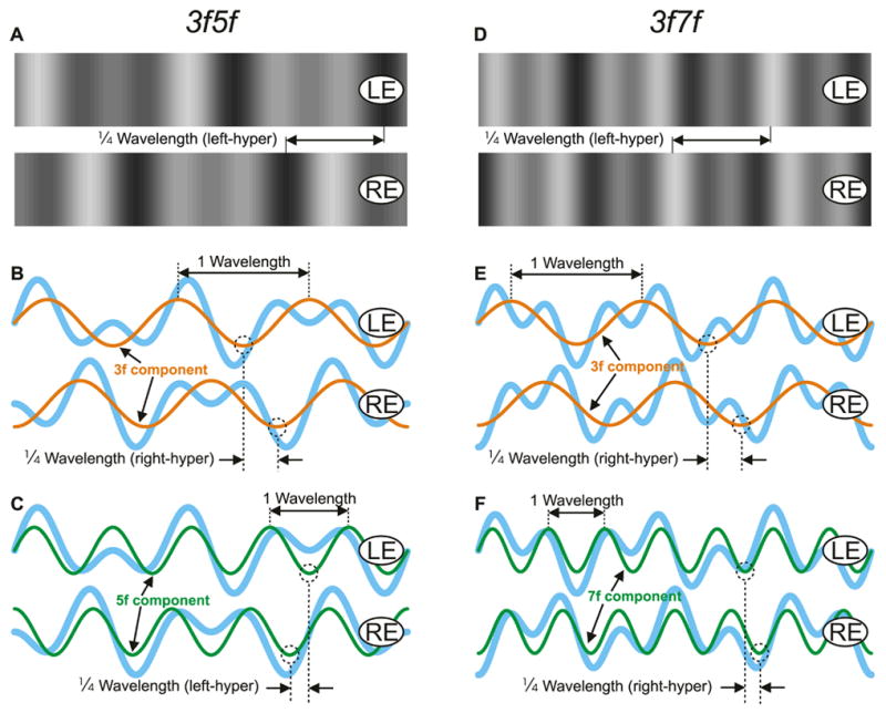
Horizontal dual-grating stimuli with competing vertical disparities. Left column: the “LH5f+RH3f stimulus”. Right column: the “RH7f+RH3f stimulus”. Note that the stimuli have been rotated clockwise 90° so that within each column the tops of the patterns are depicted on the right and the bottoms of the patterns are depicted on the left. (A, D): x-y plots of the luminance, showing the horizontal grating pairs as seen by the left (labeled, LE) and right (labeled, RE) eyes when presented with a ¼-wavelength phase difference that has left-hyper disparity (one complete wavelength is shown). (B, C, E, F): the luminance profiles of the dual grating stimuli are shown in pale blue line, with those of the 3f component superimposed in orange line (B, E), and the 5f (C) and the 7f (F) components superimposed in green line. The ¼-wavelength phase differences of the 3f components (right-hyper disparity), the 5f component (left-hyper disparity), and the 7f component (right-hyper disparity) are indicated in dashed line.

2.1.3. Eye-movement recording

The horizontal and vertical positions of both eyes were recorded with an electromagnetic induction technique (Robinson, 1963) using scleral search coils embedded in silastin rings (Collewijn, Van Der Mark & Jansen, 1975), and each was sampled at 1-ms intervals as described by Yang, FitzGibbon and Miles (2003).

2.1.4. Procedures

All aspects of the experimental paradigms were controlled by three PCs, which communicated via Ethernet using the TCP/UDP/IP protocol. One of the PCs was running a Real-time EXperimentation software package (REX) developed by Hays, Richmond and Optican (1982), and provided the overall control of the experimental protocol as well as acquiring, displaying, and storing the eye-movement data. The other two PCs were running Matlab subroutines, utilizing the Psychophysics Toolbox extensions (Brainard, 1997; Pelli, 1997), and generated the visual stimuli upon receiving a start signal from the REX machine.

At the beginning of each recording session, the horizontal and vertical signals from each eye coil were calibrated separately by having the subject fixate monocular targets presented at known eccentricities along the horizontal and vertical meridians. After completing the calibrations, the experiment proper began. At the beginning of each trial the subject was instructed to fixate a binocular central target cross (2° high × 10° wide × 0.21° thick) that was either black or white on alternate trials and appeared at the center of an otherwise uniform grey screen. After the subject’s two eyes had each been positioned within 2° of the center of its fixation cross and no saccades had been detected (using an eye velocity threshold of 18°/s) for a randomized period of 800 to 1100 ms both crosses disappeared and were immediately replaced by grating patterns (randomly selected from a lookup table); these patterns were identical for the two eyes except for a phase difference of ¼-wavelength, and filled the screens for 200 ms. At this point the screens were blanked, marking the end of the trial. At all times, the mean luminance was 38.7 cd/m². After an inter-trial interval of 500 ms, the binocular fixation cross reappeared, commencing a new trial. The subjects were asked to refrain from blinking or making any saccades except during the inter-trial intervals but were given no instructions relating to the disparity stimuli. If no saccades were detected during the period of the trial, then the data were stored on a hard disk; otherwise, the trial was aborted and subsequently repeated. Each block of trials had 90 randomly interleaved stimulus combinations: 3 grating patterns, each with 15 contrasts (for the single-grating 3f and 5f stimuli) or contrast ratios (for the dual-grating 3f5f stimuli), and the disparity could have 2 signs. Data were collected over several sessions until each condition had been repeated an adequate number of times to permit good resolution of the responses (through averaging). The actual numbers of trials will be given in the Results.

2.1.5. Data analysis

The horizontal and vertical eye-position measures obtained during the calibration procedure were each fitted with second-order polynomials which were then used to linearize the corresponding eye-position data recorded during the experiment proper. The linearized eye-position measures were smoothed with a 6-pole Butterworth filter (3 dB at 45 Hz) and then mean temporal profiles were computed for each stimulus condition. Trials with saccadic intrusions (that had failed to reach the eye-velocity threshold of 18°/s during the experiment) were deleted. We used the convention that rightward and upward deflections of the stimuli or eyes were positive. The vertical (horizontal) vergence angle was computed by subtracting the vertical (horizontal) position of the right eye from the vertical (horizontal) position of the left eye. This meant that left-sursumvergence and convergence had positive signs. The initial vergence responses in each stimulus condition were quantified by measuring the changes in the vergence position measures over the 70-ms time periods commencing 60 ms after the onset of the disparity stimuli. The minimum latency of vergence was ~65–70 ms from the first appearance of the disparity stimuli so that these vergence-response measures were restricted to the initial open-loop period.

2.2. Results

The direction of the initial vergence responses obtained with the pure sine-wave stimuli was always as expected of a negative-feedback mechanism operating to eliminate the ¼-wavelength phase difference, consistent with a sensing mechanism that gives greatest weight to the nearest neighbor binocular matches (cf., Sheliga et al., 2006a). This is apparent from the sample mean vergence velocity profiles in Fig. 2 obtained from subject FAM: when the sign of the disparity stimuli was defined by the ¼-wavelength phase differences, left-hyper disparities resulted in left sursumvergence (LH5f data in Fig. 2A; LH3f data in Fig. 2D) and right-hyper disparities resulted in right sursumvergence (RH3f data in Fig. 2B; RH5f data in Fig. 2E), with minimum onset latencies <70 ms. It is also evident that there was strong dependence on the contrast of the gratings over the limited range examined: see the numbers to the right side of the traces in Fig. 2 (each is aligned with the peak response and indicates the stimulus contrast used to generate the associated trace). Figure 3 indicates that the change-in-vergence-position measures for these data showed a nearly linear dependence on the contrast: the data obtained with the 5f stimuli are shown in green circles (left-hyper data labeled LH5f in Fig. 3A; right-hyper data labeled RH5f in Fig. 3B), and the data obtained with the 3f stimuli are shown in orange circles (right-hyper data labeled RH3f in Fig. 3A; left-hyper data labeled LH3f in Fig. 3B). The r² values for the linear regressions in Fig. 3 ranged from 0.939 to 0.957, and the regression coefficients are listed in Table 1, which includes the data for all subjects. Note that the data obtained from subject JRC with left-hyper stimuli showed very weak dependence on contrast and, because this subject also showed unusually strong vertical “default” vergence responses in the right-sursumvergent direction (Busettini et al., 2001), the latter were often greater than the responses to the left-hyper disparity stimuli.²

Fig. 2.

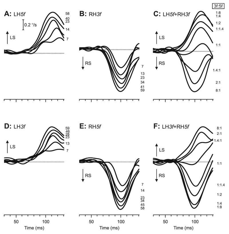
The initial vertical vergence responses to dual-grating stimuli with two disparities of opposite sign: dependence on contrast and Contrast Ratio (sample responses from subject FAM). Mean vergence velocity profiles (n=90–100) over time—derived from mean vergence position signals by computing the two-point (15 ms apart) central difference between the symmetric weight moving averages (15 points) of the vergence-position sample (Usui & Amidror, 1982)—are shown. (A): Responses to LH5f stimuli, in which the pure 5f stimuli had left-hyper disparity. (B): Responses to RH3f stimuli, in which the pure 3f stimuli had right-hyper disparity. (C): Responses to LH5f+RH3f dual-grating stimuli, in which the 5f component had left-hyper disparity and the 3f component had right-hyper disparity. (D): Responses to LH3f, in which the pure 3f stimuli had left-hyper disparity. (E): Responses to RH5f stimuli, in which the pure 5f stimuli had right-hyper disparity. (F): LH3f+RH5f dual-grating stimuli, in which the 3f component had left-hyper disparity and the 5f component had right-hyper disparity. The numbers to the right of the traces, each located at the level of the relevant peak in the profile, indicate the contrast (single gratings) and the Contrast Ratio, 3f:5f (dual gratings). Left sursumvergent responses have positive sign (upward deflections, labeled LS), and right sursumvergent responses have negative sign (downward deflections, labeled RS).

Fig. 3.

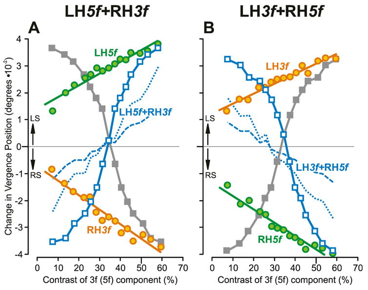
The initial vertical vergence responses to dual-grating stimuli with two disparities of opposite sign: dependence on contrast (mean vergence position measures for subject FAM). (A): Responses when pure 5f stimuli had left-hyper disparity (green circles, labeled LH5f), pure 3f stimuli had right-hyper disparity (orange circles, labeled RH3f), and dual-grating stimuli had a 5f component with left-hyper disparity and a 3f component with right-hyper disparity (blue open squares, labeled LH5f+RH3f, plotted with respect to the contrast of the 5f component; closed grey squares are the same data plotted with respect to the contrast of the 3f component). (B): Responses when pure 3f stimuli had left-hyper disparity (orange circles, labeled LH3f), pure 5f stimuli had right-hyper disparity (green circles, labeled RH5f), and dual-grating stimuli had a 3f component with left-hyper disparity and a 5f component with right-hyper disparity (blue open squares, labeled LH3f+RH5f, plotted with respect to the contrast of the 5f component; closed grey squares are the same data plotted with respect to the contrast of the 3f component). Blue dotted lines are the vector-sum predictions, and blue dashed lines are the vector-average predictions, each plotted with respect to the contrast of the 5f component. Left sursumvergent responses (labeled, LS) have positive sign, and right sursumvergent responses (labeled, RS) have negative sign. Data points are means of 90–100 samples, and SD’s ranged 0.008–0.014°.

Table 1.

Vertical vergence responses to single-grating disparity stimuli: dependence of the vertical change-in-vergence-position measures on the contrast (linear regression coefficients).

Subject	Stimulus	slope	offset	r2
BMS	LH3f	0.053	0.013	0.981
	RH3f	−0.047	−0.009	0.978
	LH5f	0.050	0.013	0.990
	RH5f	−0.044	−0.011	0.973
FAM	LH3f	0.037	0.012	0.943
	RH3f	−0.054	−0.007	0.957
	LH5f	0.043	0.014	0.939
	RH5f	−0.050	−0.013	0.948
JRC	LH3f	0.007	−0.004	0.951
	RH3f	−0.039	−0.013	0.540
	LH5f	0.006	−0.004	0.593
	RH5f	−0.035	−0.017	0.958

Not surprisingly, the initial vergence responses elicited by the 3f5f stimuli, in which the 3f and 5f components had opposite disparity, depended critically on the relative contrast of those components. This can be seen in Fig. 2C (and F), for which the 5f component was always subject to the same left-hyper (right-hyper) ¼-wavelength disparity while the 3f component was always subject to the same right-hyper (left-hyper) ¼-wavelength disparity, and the family of traces shows the data for a range of relative contrasts, which are indicated by the contrast ratios, 3f:5f, shown to the right of the traces. Note that the total contrast of the 3f5f stimuli was always 64%, so that increases in the contrast of one component were offset by decreases in the contrast of the other. When the contrast ratio strongly favored the 5f component (e.g., 3f:5f=1:8), the response was very similar to that elicited by the highest-contrast pure 5f stimulus (left-sursumvergence in Fig. 2A, C; right-sursumvergence in Fig. 2E, F), and when the contrast ratio favored the 3f component (e.g., 8:1), the response was very similar to that elicited by the highest-contrast pure 3f stimulus (right-sursumvergence in Fig. 2B, C, left-sursumvergence in Fig. 2D, F). The clear suggestion here is that the component with the lower contrast has little or no influence. Of course, intermediate contrast ratios resulted in intermediate responses as the influence of one component waxed while the other waned.

The change-in-vergence-position measures for the 3f5f data in Fig. 2 are plotted in Fig. 3 and indicate that the responses to the dual gratings could not be predicted by a simple vector sum or average of the responses to the two components when each was applied in isolation. Note that the data from Fig. 2A–C are plotted in Fig. 3A and the data from Fig. 2D–F are plotted in Fig. 3B. Also note that the responses to the 3f5f stimuli are each plotted twice in Fig. 3: first, as a function of the contrast of the 5f component (blue open squares), to show how closely they approached the data obtained with the pure 5f stimuli (green circles) when the 5f component had high contrast; second, as a function of the contrast of the 3f component (closed grey squares), to show how closely they approached the data obtained with the pure 3f stimuli (orange circles) when the 3f component had high contrast. Thus, the data obtained with the dual-grating 3f5f stimuli show a slightly sigmoidal dependence on contrast in Fig. 3. If the responses here had been a simple vector sum then, to the extent that the responses to the pure 3f and 5f stimuli showed a linear dependence on contrast, the 3f5f data plots in Fig. 3 would also have shown a roughly linear dependence on contrast and would not have fully merged with the pure 5f or 3f data: see the blue dotted lines in Fig. 3 indicating the vector sum of the responses to pure 5f and 3f stimuli whose relative contrasts matched those for the 3f5f stimuli (plotted with respect to the contrast of the 5f component). The values predicted by the vector averages of the responses to these same 5f and 3f stimuli are exactly half the values predicted by the vector sums and so deviate from the dual-grating data by an even wider margin than do the vector sum predictions: see the blue dashed lines in Fig. 3.

To quantify the transition from dominance by one component to dominance by the other, we computed the Response Ratio of Sheliga et al. (2006b) using the following expression:

$$\frac{R_{3f5f}-R_{3f}}{R_{5f}-R_{3f}}$$ (1)

where R_3f5f is the mean response to the dual-grating 3f5f stimulus when the 3f and 5f components have particular contrast values, and R_3f and R_5f are the mean responses to single-grating 3f and 5f stimuli with contrasts matching those values. To the extent that the response to the dual-grating stimulus is determined exclusively by the 5f component (i.e., R_3f5f ≈ R_5f), the value of the numerator in Expression 1 will approach the value of the denominator and the Response Ratio will therefore approach unity. To the extent that the response to the dual-grating stimulus is determined exclusively by the 3f component (i.e., R_3f5f ≈ R_3f), the value of the numerator in Expression 1 will approach zero and the Response Ratio will therefore also approach zero. In Fig. 4A, the 3f5f data of subject FAM in Fig. 3 have been replotted to show the Response Ratios as a function of the Contrast Ratio (on a log scale). It is now clear that when the Contrast Ratios were less than ~0.4, the 5f component was almost totally dominant and when the contrast ratios were greater than ~2.5, the 3f component was almost totally dominant. Thus, when the Contrast Ratio was high or low only one component was effective (winner-take-all) and the transition from one extreme to the other was rather abrupt. This is all in stark contrast to the vector-sum predictions (thin lines in Fig. 4A), and the vector-average predictions deviate even further from the real data, having a Response Ratio that is always 0.5 (not shown in Fig. 4A).

Fig. 4.

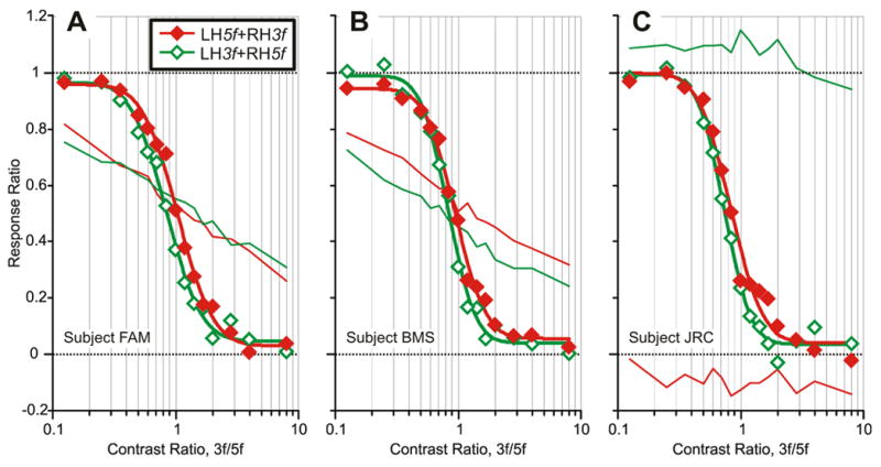
The initial vertical vergence responses to dual-grating stimuli with two disparities of opposite sign: dependence of the Response Ratio on the Contrast Ratio (data for 3 subjects). Plots are based on data obtained with the LH5f+RH3f stimuli (red filled diamonds) and LH3f+RH5f stimuli (green open diamonds). Continuous smooth curves are best-fit Cumulative Gaussian functions. Thin lines are the vector-sum predictions (red: LH5f+RH3f stimuli; green: LH3f+RH5f stimuli). (A): subject FAM (n=90–100 response samples per stimulus). (B): subject BMS (n=50–55). (C): subject JRC (n=104–112).

The data obtained from the other two subjects with the dual-grating stimuli showed very similar nonlinear dependencies on Contrast Ratio with relatively abrupt transitions: see Figs. 4B, C. The data of subject JRC (Fig. 4C) are particularly interesting because this subject’s responses to both left-hyper and right-hyper stimuli were offset in the right-sursumvergence direction resulting in hugely different vector-sum predictions for the two 3f5f data sets that both lay outside the range of the “real” 3f5f data. Nonetheless, the dependence of the Response Ratios on the Contrast Ratio in this subject were little different from those in the other two subjects.

To obtain a quantitative estimate of the abruptness of the transitions in Fig. 4, each of the 2 data sets for each subject was fitted with a Cumulative Gaussian function using a least squares criterion: see the smooth curves in these graphs and their parameters in Table 2. The r² values for these fits averaged 0.993 and were never less than 0.984, indicating that they provide a very adequate description of these data. The amplitudes of the Cumulative Gaussians were always slightly less than unity (mean, 0.93) and their Standard Deviations (SDs) ranged from 0.17 to 0.23 (mean±SD, 0.20±0.03). We also wanted to obtain an estimate of how different the contrasts of the two components of the 3f5f stimuli had to be for one of the components to effectively lose its influence. For this we used the Cumulative Gaussian to determine a Transition Zone, which we defined as the range of Contrast Ratios over which the Response Ratio ranged from 0.05 to 0.95: see the “5%” and “95%” listings in Table 2. On average—based on the mean Cumulative Gaussian for all data from all subjects—this Transition Zone extended from 0.40 to 1.88. Thus, if the two sine waves were of similar efficacy when of equal contrast and applied singly, then when combined as in our dual gratings, on average, a 2.2-fold difference in contrast sufficed for the one with the lower contrast to almost totally lose its influence.³

Table 2.

Vertical vergence responses to the dual-grating disparity stimuli: dependence of the Response Ratio on the Contrast Ratio (parameters of best-fit Cumulative Gaussian).

Subject	Stimulus	SD	r2	5%	95%
BMS	LH5f+RH3f	0.20	0.994	1.99	0.45
	LH3f+RH5f	0.18	0.991	1.61	0.42
FAM	LH5f+RH3f	0.23	0.994	2.48	0.43
	LH3f+RH5f	0.23	0.992	1.98	0.35
JRC	LH5f+RH3f	0.21	0.984	1.82	0.38
	LH3f+RH5f	0.17	0.995	1.41	0.38
Mean± SD		0.20± 0.03	0.993±0.000	1.88±0.37	0.40±0.04

5%, 95% refer to the Contrast Ratios when the best-fit Cumulative Gaussian has values of 0.05 and 0.95, respectively.

2.3. Discussion of Experiment 1

The data in Fig. 4 indicate that when two superimposed horizontal sine-wave gratings of different spatial frequency had vertical disparities of opposite sign, the resulting vertical vergence responses depended critically on the relative contrasts of those two sine waves, and this dependence was highly nonlinear, involving a relatively abrupt transition from dominance by one sine wave to dominance by the other: winner-take-all. In fact, the dominance was almost complete with a 2.2-fold difference in contrast. We have previously reported that, when confronted with two sine-wave gratings moving in opposite directions, the OFR—a short-latency ocular tracking response to large-field motion—shows similar nonlinear interactions with slightly more abrupt transitions, so that on average a 1.8-fold difference in contrast is sufficient to render the OFR essentially unresponsive to the motion of the component with the lower contrast (Sheliga et al., 2006b).

Following the lead of previous authors, who reported winner-take-all ocular tracking responses with competing visual motions and attributed them to mutual inhibition between motion-sensitive channels (Ferrera, 2000; Ferrera & Lisberger, 1995; 1997; Recanzone & Wurtz, 1999; Sheliga et al., 2006b), we invoke mutual inhibition between disparity-sensitive channels with preferences for disparities of opposite sign to account for the nonlinear interactions in our present data. In fact, there is psychophysical evidence that horizontal disparity signals are processed by multiple narrowly-tuned channels or filters (Stevenson, Cormack, Schor & Tyler, 1992) that display mutual inhibition (Cormack, Stevenson & Schor, 1993). In its most extreme form, the mutual inhibition might be so powerful that the response on any given trial is exclusively driven by only one of the two components. This seems likely to have been the situation when the Contrast Ratio was outside the Transition Zone and resulted in Response Ratios close to either zero or unity. However, it is possible that a winner-take-all arrangement always prevailed—even when the Contrast Ratio was within the Transition Zone—but is not evident from plots like those in Fig. 4 because only mean Response Ratios are plotted. For example, a mean Response Ratio of 0.5 could result if vergence was effectively driven exclusively by the 5f component in half of the trials and exclusively by the 3f component in the other half of the trials. If this were the case, then we might expect the distributions of the individual vergence responses to a given 3f5f stimulus to be bimodal inside the Transition Zone and unimodal outside. In examining this possibility we will first consider an example of a response distribution close to the center of the Transition Zone: see Fig. 5. The histograms in Fig. 5A show the distributions of the initial DVRs obtained from subject FAM using pure RH3f stimuli (orange plot) and pure LH5f stimuli (green plot) each of contrast 34.5%, and dual-grating RH3f+LH5f stimuli (blue plot) whose 3f and 5f components also each had contrasts of 34.5%. The best-fit Gaussians for those three distributions are shown in continuous thick line and have r² values of 0.956, 0.879 and 0.925, respectively, indicating that all were unimodal. Further, the SDs of these distributions (0.010°, 0.011°, 0.011°, respectively) were not significantly different (Fischer test).⁴ This would seem to imply that the winner-take-all situation does not operate in the Transition Zone, and in order to confirm this we ran a simulation. For this, we used the mean responses to the three stimuli and Expression 1 to estimate the Response Ratio (0.51), and then simulated the response distribution predicted by the winner-take-all model for the LH5f+RH3f stimuli by summing the response distributions obtained with the pure LH5f and RH3f stimuli, weighted in accordance with this Response Ratio: see the grey histogram in Fig. 5B labeled, “LH5f+RH3f”. It is clear from this that the simulated “LH5f+RH3f” dual-grating response distribution was indeed bimodal and extended well beyond the extremes of the real unimodal LH5f+RH3f response distribution, which is replotted in Fig. 5B (in blue) to facilitate the comparison. The differences between the distributions of the “real” and the “simulated” responses in Fig. 5B were significant at the 0.01 level on the Kolmogorov-Smirnov two-sample test. That the data in Fig. 5 were typical of the distributions at the center of the Transition Zone was apparent from the data obtained from all three subjects. Thus, the r² values for the best-fit Gaussians to the distributions of those responses to the dual-grating 3f5f stimuli for which the Response Ratio was closest to 0.5 (the center of the Transition Zone) ranged from 0.859 to 0.970 (mean, 0.920). Further, in 11/12 cases, the SDs of the 3f5f distributions near the center of the Transition Zone were not significantly different from the SDs of the distributions for which the Response Ratios were closest to zero or unity (Fischer test).⁵ Finally, the distributions of the “real” and the “simulated” responses to the 3f5f stimuli for all data obtained from all three subjects were significantly different when the Response Ratios were closest to 0.5 but not when they were closest to zero or unity (Kolmogorov-Smirnov two-sample test). These findings are all consistent with the idea that vector sum/averaging prevails near the center of the Transition Zone and winner-take-all prevails outside this Zone.

Fig. 5.

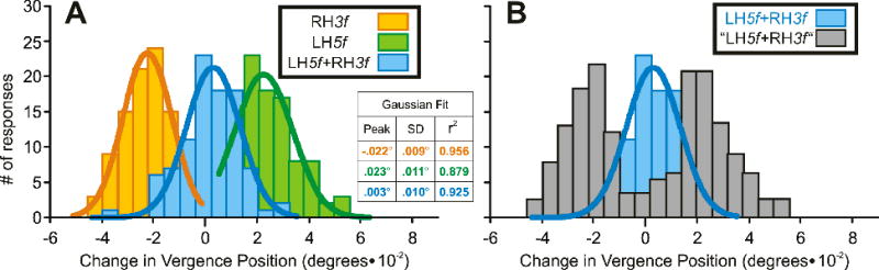
The initial vertical vergence responses to dual-grating stimuli with two disparities of opposite sign: simulation of the response distributions near the center of the Transition Zone based on the winner-take-all model (sample data from subject FAM). (A): Histograms of the distributions of the response measures (n=94–97) obtained when pure 3f stimuli of contrast 34.5% had right-hyper disparity (orange plot, labeled RH3f), pure 5f stimuli of contrast 34.5% had left-hyper disparity (green plot, labeled LH5f), and dual-grating stimuli had 3f and 5f components with matching disparities and contrasts (blue plot, labeled LH5f+RH3f); smooth curves are best-fit Gaussian functions. (B): Histogram of the simulated LH5f+RH3f distribution obtained by summing the measured distributions for the pure RH3f stimuli and the pure LH5f stimuli but weighted in accordance with the measured Response Ratio of 0.51 (grey plot, labeled “LH5f+RH3f”); the data actually obtained with the dual-grating stimuli are replotted here to facilitate easy comparison (blue plot, labeled LH5f+RH3f). Histograms were binned using custom Matlab subroutines in which the optimal bin width for each individual distribution was given by 2(IQR) N^−1/3, where IQR is the interquartile range (the 75th percentile minus the 25th percentile) and N is the number of samples. The sole exception to this was the “simulated” distribution in B, for which the bin width was made the same as for the “real” distribution in B.

Our previous study on the OFRs to competing motion stimuli also concluded that a winner-take-all situation prevailed outside the Transition Zone and vector sum/averaging within it (Sheliga et al., 2006b). In addition, that study was able to fully account for this nonlinear behavior (mean r², 0.993) using a contrast-weighted-average model with just two free parameters (cf., Krommenhoek & Wiegerinck, 1998; McGowan, Kowler, Sharma & Chubb, 1998; Port & Wurtz, 2003; Recanzone & Wurtz, 1999). We used this same approach on our present data by determining how the 3f5f data like those in Fig. 3 (describing the dependence of the change-in-vergence-position measures on the contrast of the 5f component) were fitted by the following Contrast-Weighted-Average model:

$${\overrightarrow{R}}_{3f5f}=\frac{{\left(C_{3f}\right)}^{n_{3f}}}{{\left(C_{3f}\right)}^{n_{3f}}+{\left(C_{5f}\right)}^{n_{5f}}}{\overrightarrow{R}}_{3f}+\frac{{\left(C_{5f}\right)}^{n_{5f}}}{{\left(C_{3f}\right)}^{n_{3f}}+{\left(C_{5f}\right)}^{n_{5f}}}{\overrightarrow{R}}_{5f}$$ (2)

where R⃗_{3 f 5 f} is the simulated DVR to a given 3f5f stimulus whose two components have contrasts of C_{3 f} and C_{5 f}, respectively; R⃗_{3 f} and R⃗_{5 f} are the measured DVRs to pure 3f and 5f stimuli, respectively, with contrasts of C_{3 f} and C_{5 f}, respectively; n_3f and n_5f are two free parameters that reflect the efficacies of the 3f and 5f components, respectively, of the given 3f5f stimulus and thereby determine the abruptness of the transition. The least squares best-fit values of the n_3f and n_5f parameters, together with the r² values indicating the goodness of the fits, for all of the dual-grating data like those in Fig. 3 are listed in Table 3. The r² values ranged from 0.990 to 0.997, indicating that Equation 2 provided a very good and complete description of the data. The exponents provide an estimate of the strengths of the mutual inhibition between the two sine-wave gratings, and averaged 2.99 (n_5f) and 3.40 (n_3f). The corresponding values for the OFR were 5.43 and 5.20 (Sheliga et al., 2006b). In sum, the Contrast-Weighted-Average model, with only two free parameters, provided a very good description of our data and a quantitative estimate of the strength of the nonlinear interactions.

Table 3.

Vertical vergence responses to dual-grating disparity stimuli: dependence of the vertical change-in-vergence-position measures on the contrast of the 5f component (parameters of the best-fit Contrast-Weighted-Average model).

Subject	Stimulus	n3f	n5f	r2
BMS	LH5f+RH3f	2.85	2.99	0.994
	LH3f+RH5f	3.44	4.00	0.994
FAM	LH5f+RH3f	2.84	2.76	0.996
	LH3f+RH5f	2.55	2.96	0.995
JRC	LH5f+RH3f	2.75	3.16	0.990
	LH3f+RH5f	3.49	4.54	0.997
Mean± SD		2.99±0.39	3.40±0.71	0.994±0.002

Responses were fitted with Equation 2; n_3f and n_5f are the two free parameters.

We also fitted the data like those in Fig. 3 with a Response-Weighted-Average model in which vergence response measures were substituted for the contrast values in Expression 2. Because the DVR shows a linear dependence on contrast over the range examined, one might expect that the Response-Weighted-Average model would also provide a good approximation to the data. This was indeed the case for the data of subjects FAM and BMS (r² values ranged from 0.976 to 0.986) but not for the data of subject JRC (r² values, 0.343 and 0.526) whose responses to both left-hyper and right-hyper stimuli were offset in the right-sursumvergence direction. Thus, only the Contrast-Weighted-Average model provided a good fit to all of the data, consistent with nonlinear interactions between the mechanisms sensing the competing disparities, i.e., the interactions occur at the sensory—rather than the motor—level.

In order for the postulated mutual inhibition generated by the higher contrast component to totally suppress even the earliest vergence responses generated by the lower contrast component, the former must have the shorter latency. There is abundant evidence that higher contrast stimuli elicit activity in striate cortex at shorter latencies than low contrast stimuli (e.g., Albrecht, 1995; Albrecht, Geisler, Frazor & Crane, 2002; Carandini & Heeger, 1994; Carandini, Heeger & Movshon, 1997; Gawne, Kjaer & Richmond, 1996). We examined this issue by comparing the latencies of the DVRs to the highest contrast 3f stimuli with those to the lowest contrast 5f stimuli (and vice versa), as well as the latencies of the DVRs to the second-highest contrast 3f stimuli with those to the second-lowest contrast 5f stimuli (and vice versa). These stimulus pairs corresponded to the components of the dual-grating stimuli that showed the most robust winner-take-all responses and revealed a strong tendency for the DVRs to the grating with the higher contrast to have the lower latency but, importantly, the situation was reversed for 6/23 stimulus pairs. This is again consistent with the idea that the nonlinear interactions occur early in the visuomotor pathways.

3. Experiment 2: Initial horizontal vergence responses to the 3f5f stimulus and their dependence on the relative contrast of the two components

The stimuli used in this experiment were similar to those in Experiment 1 except that their orientations were orthogonal: we recorded the initial horizontal vergence responses that were elicited when horizontal ¼-wavelength disparities of opposite sign were applied simultaneously to two superimposed vertical sine-wave gratings whose spatial frequencies were in the ratio 3:5. We varied the relative contrast of the two gratings and again found evidence of nonlinear interactions but these were weaker than in Experiment 1—often appreciably so—and showed much more inter-subject variability.

3.1. Methods

Most of the methods, including the subjects, were identical to those used in Experiment 1, and only those that were different will be described here.

3.1.1. Visual display

Visual images again consisted of one-dimensional grating patterns like those in Experiment 1 except that, 1) they were vertically oriented, and 2) the spatial frequencies used for the 3f and 5f stimuli were: 0.264 and 0.440 cycles/°, respectively, for subject BMS; 0.272 and 0.453 cycles/°, respectively, for subject FAM; 0.335 and 0.559 cycles/°, respectively, for subject JRC. Images were identical for the two eyes except for a horizontal phase difference that was ¼ of the wavelength and this defined the binocular disparity stimulus. For the 3f5f stimuli, this meant that the two component sine waves each had a disparity of ¼ its own wavelength but these were of opposite sign: a 3f component with crossed disparity was combined with a 5f component that had uncrossed disparity (the X3f+UX5f stimulus) and vice versa (the X5f+UX3f stimulus). Contrasts (and so Contrast Ratios) were as in Experiment 1.

3.2. Results

Compared with the vertical vergence data, the horizontal vergence data were much less consistent, showing much greater trial-by-trial response variability with a given stimulus as well as substantial inter-subject variability in the extent of the nonlinear interactions uncovered by the competing disparities, and these interactions were often less potent than those seen with the vertical disparity stimuli. Even the mean horizontal vergence response profiles showed appreciably greater residual noise than the equivalent vertical vergence data although often based on a substantially larger data set. The general layout of the Results, including the tables and figures, has the same format as for Experiment 1.

That the direction of the initial horizontal vergence responses obtained with the pure sine-wave stimuli was always as expected of a negative-feedback mechanism operating to eliminate the ¼-wavelength phase difference is apparent from the sample vergence velocity traces from subject FAM in Fig. 6: when the sign of the disparity stimuli was defined by the ¼-wavelength phase differences, crossed disparities resulted in convergence (X5f data in Fig. 6A; X3f data in Fig. 6D) and uncrossed disparities resulted in divergence (UX3f data in Fig. 6B; UX5f data in Fig. 6E), with minimum onset latencies <70 ms (cf., Sheliga et al., 2006a). The change-in-vergence-position measures again showed a roughly linear dependence on contrast: see Fig. 7, in which the data obtained with the 5f stimuli are shown in green circles (data obtained with crossed disparities labeled X5f in Fig. 7A; data obtained with uncrossed disparities labeled UX5f in Fig. 7B), and the data obtained with the 3f stimuli are shown in orange circles (uncrossed data labeled UX3f in Fig. 7A; crossed data labeled X3f in Fig. 7B). The r² values for the linear regressions in Fig. 7 ranged from 0.901 to 0.964, and the regression coefficients are listed in Table 4, which includes the data for all subjects.

Fig. 6.

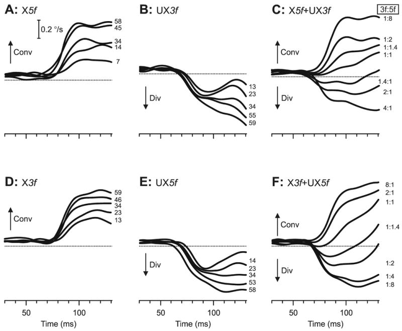
The initial horizontal vergence responses to dual-grating stimuli with two disparities of opposite sign: dependence on contrast and Contrast Ratio (sample responses from subject FAM). Mean vergence velocity profiles (each based on responses to 185–197 stimuli) over time, derived as described in the legend to Fig. 2. (A): X5f stimuli, in which the pure 5f stimuli had crossed disparity. (B): UX3f stimuli, in which the pure 3f stimuli had uncrossed disparity. (C): X5f+UX3f stimuli, dual-grating stimuli in which the 5f component had crossed disparity and the 3f component had uncrossed disparity. (D): X3f stimuli, in which the pure 3f stimuli had crossed disparity. (E): UX5f stimuli, in which the pure 5f stimuli had uncrossed disparity. (F): X3f+UX5f stimuli, dual gratings in which the 3f component had crossed disparity and the 5f component had uncrossed disparity. The numbers to the right of the traces, each located at the level of the relevant peak in the profile, indicate the contrast (single gratings) and the Contrast Ratio, 3f:5f (dual gratings). Convergent responses have positive sign (upward deflections, labeled Conv), and divergent responses have negative sign (downward deflections, labeled Div).

Fig. 7.

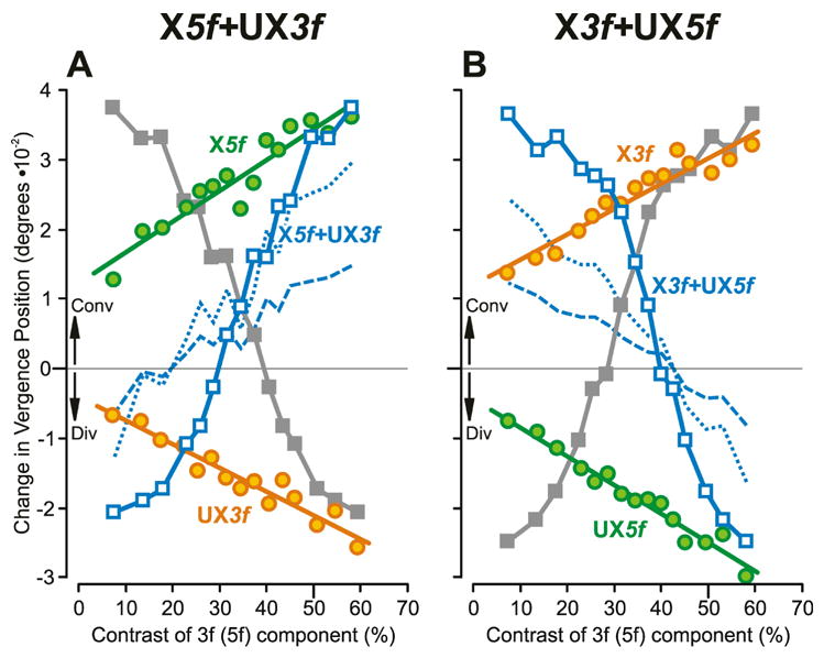
The initial horizontal vergence responses to dual-grating stimuli with two disparities of opposite sign: dependence on contrast (mean vergence position measures for subject FAM). (A): Responses when pure 5f stimuli had crossed disparity (green circles, labeled X5f), pure 3f stimuli had uncrossed disparity (orange circles, labeled UX3f), and dual-grating stimuli had a 5f component with crossed disparity and a 3f component with uncrossed disparity (blue open squares, labeled X5f+UX3f, plotted with respect to the contrast of the 5f component; closed grey squares are the same data plotted with respect to the contrast of the 3f component). (B): Responses when pure 3f stimuli had crossed disparity (orange circles, labeled “X3f”), pure 5f stimuli had uncrossed disparity (green circles, labeled UX5f), and dual gratings had a 3f component with crossed disparity and a 5f component with uncrossed disparity (blue open squares, labeled X3f+UX5f, plotted with respect to the contrast of the 5f component; closed grey squares are the same data plotted with respect to the contrast of the 3f component). Blue dotted lines are the vector-sum predictions, and blue dashed lines are the vector-average predictions, each plotted with respect to the contrast of the 5f component. Convergent responses (Conv) have positive sign, and divergent responses (Div) have negative sign. Data points are means of 185–197 samples and SD’s ranged 0.013–0.029°.

Table 4.

Horizontal vergence responses to single-grating disparity stimuli: dependence of the horizontal change-in-vergence-position measures on the contrast (linear regression coefficients).

Subject	Stimulus	slope	offset	r2
BMS	X3f	0.032	0.006	0.921
	UX3f	−0.038	−0.009	0.895
	X5f	0.038	0.010	0.908
	UX5f	−0.019	−0.008	0.830
FAM	X3f	0.037	0.012	0.927
	UX3f	−0.034	−0.004	0.919
	X5f	0.044	0.012	0.901
	UX5f	−0.042	−0.004	0.964
JRC	X3f	0.016	0.006	0.946
	UX3f	−0.032	0.001	0.707
	X5f	0.026	0.005	0.951
	UX5f	−0.024	−0.002	0.920

The initial vergence responses elicited by the dual-grating 3f5f stimuli again depended on the relative contrasts of the two components (see sample data from subject FAM in Fig. 6C, F), so that when the contrast ratio strongly favored the 5f component, the response was very similar to that elicited by the 5f stimulus alone (convergence in Fig. 6C, divergence in Fig. 6F), and when the contrast ratio favored the 3f component, the response was very similar to that elicited by the 3f stimulus alone (divergence in Fig. 6C, convergence in Fig. 6F). The change-in-vergence-position measures for these data are plotted in Fig. 7A, B and show a clear similarity with the vertical vergence data in Fig. 3, consistent with nonlinear interactions between the responses to the two competing stimuli. Although these horizontal vergence responses show somewhat more scatter than the vertical vergence data, it is nonetheless clear that the 3f5f data tend to deviate away from the vector-sum predictions (blue dotted lines in Fig. 7), in the direction of the data obtained with the pure 3f or 5f stimuli as the contrast of one component increasingly exceeded that of the other component. As for the vertical data in Fig. 3, the values predicted by the vector averages of the responses to the 5f and 3f stimuli deviated from the dual-grating data by an even wider margin than did the vector-sum predictions: see the blue dashed lines in Fig. 7. When the 3f5f data in Fig. 7 were replotted as Response Ratios versus the Contrast Ratio (Fig. 8A), the transitions from dominance by the 5f component—when the Response Ratio approached unity—to dominance by the 3f component—when the Response Ratio approached zero—resembled those for this same subject in Fig. 4A: winner-take-all. Again, it is evident that the horizontal data in Fig. 8A show much more scatter than the vertical data of this same subject in Fig. 4A, and this is reflected in the r² values for the best-fit Cumulative Gaussian functions, which are 0.964 and 0.985 in Fig. 8A and 0.992 and 0.994 in Fig. 4A. The SDs of the Cumulative Gaussian functions for these plots (0.28 and 0.25: see Table 5) are only slightly greater than those for this same subject’s vertical data (0.23 and 0.23: see Table 1). The vertical data in Fig. 4 showed little dependence on the polarity of the disparity stimulus but this was not so of the horizontal data: the two sets of 3f5f data in Fig. 8A are clearly offset with respect to one another, the 5f component showing greater dominance with the X5f+UX3f stimulus and the 3f component showing greater dominance with the X3f+UX5f stimulus.

Fig. 8.

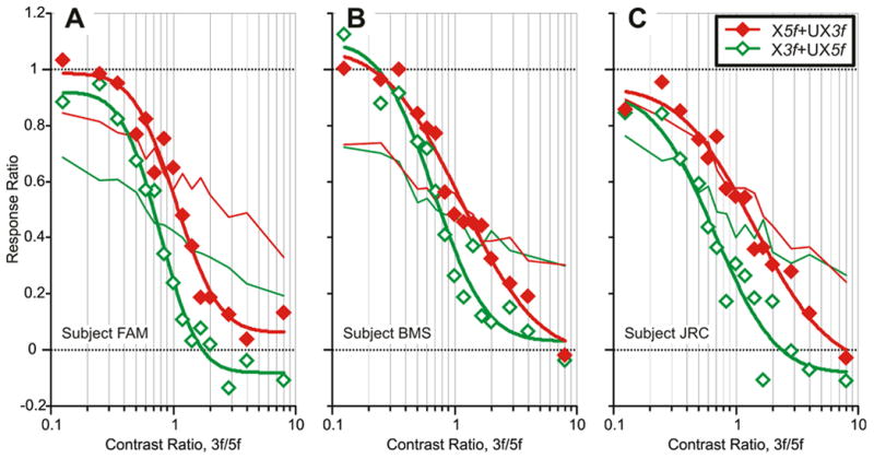
The initial horizontal vergence responses to dual-grating stimuli with two disparities of opposite sign: dependence of the Response Ratio on the Contrast Ratio (data for 3 subjects). Based on data obtained with the X5f+UX3f stimuli (filled red diamonds) and the X3f+UX5f stimuli (open green diamonds). Continuous smooth curves are best-fit Cumulative Gaussian functions. Thin lines are the vector-sum predictions (red: X5f+UX3f stimuli; green: X3f+UX5f stimuli). (A): subject FAM (n=185–197 response samples per stimulus). (B): subject BMS (n=137–145). (C): subject JRC (n=182–198).

Table 5.

Horizontal vergence responses to the dual-grating stimuli: dependence of the Response Ratio on the Contrast Ratio (parameters of best-fit Cumulative Gaussian).

Subject	Stimulus	SD	r2	5%	95%
BMS	X5f+UX3f	0.49	0.968	7.23	0.18
	X3f+UX5f	0.34	0.956	2.44	0.19
FAM	X5f+UX3f	0.28	0.964	3.03	0.36
	X3f+UX5f	0.25	0.985	1.99	0.30
JRC	X5f+UX3f	0.48	0.968	8.00	0.23
	X3f+UX5f	0.40	0.931	2.99	0.15
Mean± SD		0.37± 0.10	0.962±0.018	4.28±2.62	0.24±0.08

5%, 95% refer to the Contrast Ratios when the best-fit Cumulative Gaussian has values of 0.05 and 0.95, respectively.

The horizontal vergence data obtained from the other two subjects also showed more scatter, much more gradual transitions from one extreme to the other, and much greater dependence on the polarity of the disparity stimuli than was the case with the vertical data from these same subjects: compare Figs. 8B, C and Figs. 4B, C. Thus, based on the data obtained from all three subjects: 1) The best-fit Cumulative Gaussian functions had mean r² values of 0.962 versus 0.993 for the vertical data. 2) On average, the Transition Zone (based on the range of Contrast Ratios over which the Response Ratio ranged from 0.05 to 0.95) extended from 0.24 to 4.28, so that a 4.5-fold difference in contrast was required for the one with the lower contrast to almost totally lose its influence, which is twice that for the vertical data. 3) The horizontal vergence data obtained with the X5f+UX3f stimuli were shifted to the right⁶ of those obtained with the X3f+UX5f stimulus (Fig. 8), indicating that the crossed stimuli exerted the greater influence regardless of whether contributed by the 3f or the 5f component; in addition, the Transition Zone was consistently narrower for the data obtained with the X3f+UX5f stimuli (mean SD of Cumulative Gaussian, 0.33) than for the data obtained with the X5f+UX3f stimuli (mean SD of Cumulative Gaussian, 0.42); these dependencies on the polarity of the horizontal stimuli are in contrast with the vertical responses, which show only a very slight preference for left-hyper disparities (Fig. 4).

We again examined the 3f5f response distributions near the center of the Transition Zone and an example is shown in Fig. 9, which has the same layout as Fig. 5. The histograms in Fig. 9A show the distributions of the initial DVRs obtained from subject FAM using pure X3f stimuli (orange plot), pure UX5f stimuli (green plot), and dual-grating X3f+UX5f stimuli whose 3f and 5f components had contrasts matching those of the single-grating stimuli (blue plot). The best-fit Gaussians for those three distributions are shown in continuous thick line and all have r² values of 0.95 or greater, indicating that all distributions were unimodal. These data were typical, the r² values for the best-fit Gaussians distributions of those responses to the 3f5f stimuli for which the Response Ratios were closest to 0.5 ranging from 0.899 to 0.970 (n=6). Further, only in 1/11 cases was the SD of these distributions significantly greater than the SD of the distributions for which the Response Ratios were closest to zero or unity (Fischer test). However, the distributions of the responses to the pure 3f and 5f horizontal stimuli in Fig. 9A are clearly somewhat broader and show much more overlap than the vertical vergence data in Fig. 5A, the net result being that the “simulated” winner-take-all distribution in Fig. 9B (grey histogram) also has a unimodal distribution, (r² value for best-fit Gaussian, 0.934). This too was typical, the r² values for all of the “simulated” winner-take-all distributions from all three subjects ranging from 0.915 to 0.975 when the Response Ratios were closest to 0.5. Importantly, in all cases, these “simulated” winner-take-all distributions were significantly broader than the “real” distributions (Fischer test).

Fig. 9.

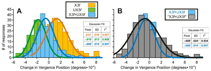
The initial horizontal vergence responses to dual-grating stimuli with two disparities of opposite sign: simulation of the response distributions near the center of the Transition Zone based on the winner-take-all model (sample data from subject FAM). (A): Histograms of the distributions of the response measures (n=191–194) obtained when pure 3f stimuli of contrast 25.4% had crossed disparity (orange plot, labeled X3f), pure 5f stimuli of contrast 42.7% had uncrossed disparity (green plot, labeled UX5f), and dual-grating stimuli had 3f and 5f components with matching disparities and contrasts (blue plot, labeled X3f+UX5f). (B): Histogram of the simulated X3f+UX5f distribution obtained by summing the measured distributions for the pure X3f stimuli and the pure UX5f stimuli but weighted in accordance with the measured Response Ratio of 0.57 (grey plot, labeled “X3f+UX5f”); the data actually obtained with the dual-grating stimuli are replotted here to facilitate easy comparison (blue plot, labeled X3f+UX5f). Smooth curves are best-fit Gaussian functions. Histograms were binned using custom Matlab subroutines as described in the legend to Fig. 5.

3.3. Discussion of Experiment 2

Compared with the vertical vergence data collected in Experiment 1, the horizontal vergence data collected in Experiment 2 generally showed much more scatter and much broader Transition Zones, as well as greater sensitivity to the polarity of the stimulus (vergence responses favoring crossed stimuli over uncrossed). The broader Transition Zones mean that in order for one of the two competing gratings to totally lose its influence (the winner-take-all situation), on average, there had to be a 4.5-fold difference in their contrasts whereas a 2.2-fold difference sufficed with vertical vergence. The “simulated” winner-take-all 3f5f response distributions near the center of the Transition Zone were always unimodal for the horizontal vergence data—a byproduct of the substantial overlap between the (broader) response distributions—but the finding that the “real” distributions were always narrower than these “simulated” ones is consistent with vector-sum/averaging.

Once more we invoke mutual inhibition between disparity-sensitive channels with preferences for disparities of opposite sign to account for the nonlinear interactions, cf., the psychophysical data of Cormack et al (1993) which led these workers to suggest that stereopsis involves “inhibition between disparity-tuned units”. We further suggest that the broader Transition Zone with horizontal vergence indicates that the inhibitory coupling is less powerful between the horizontal disparity channels than between the vertical ones. Once more, the Contrast-Weighted-Average model (Expression 2) provided an excellent fit to the data obtained with the dual-grating stimuli (mean r², 0.976): see Table 6 for a listing of the two free parameters, n_3f and n_5f, which we suggest provide an estimate of the strengths of the mutual inhibition. Comparison with the data in Table 3 indicates that these two free parameters had values substantially less than those for the vertical vergence data.

Table 6.

Horizontal vergence responses to dual-grating disparity stimuli: dependence of the horizontal change-in-vergence-position measures on the contrast of the 5f component (parameters of the best-fit Contrast-Weighted-Average model).

Subject	Stimulus	n3f	n5f	r2
BMS	X5f+UX3f	1.81	1.49	0.980
	X3f+UX5f	2.02	2.53	0.969
FAM	X5f+UX3f	2.35	2.15	0.980
	X3f+UX5f	2.53	3.66	0.983
JRC	X5f+UX3f	1.56	1.37	0.984
	X3f+UX5f	1.45	2.51	0.963
Mean± SD		1.95±0.43	2.29±0.83	0.976±0.009

Responses were fitted with Equation 2; n_3fand n_5f are the two free parameters.

4. Experiment 3: Initial vergence responses to the 3f7f stimulus and their dependence on the relative contrast of the two components

In Experiments 1 and 2 we used dual-grating stimuli whose spatial frequencies were in the ratio 3:5 and we recorded the initial vergence responses that were elicited when ¼-wavelength disparities of opposite sign were applied to the two gratings. In the present Experiment we combined two gratings whose spatial frequencies were in the ratio 3:7 and whose disparities had the same sign. In two separate studies we examined the vertical vergence elicited by vertical disparities applied to horizontal gratings (Experiment 3a) and the horizontal vergence elicited by horizontal disparities applied to vertical gratings (Experiment 3b). We again report that when the contrast of one component exceeded that of the other by a certain amount then the component with the lesser contrast lost its influence on the initial vergence responses (winner-take-all).

4.1. Methods

Most of the methods and procedures, including the subjects, were identical to those used in Experiments 1 and 2, and only those that were different will be described here.

4.1.1. Visual display

Visual images consisted of one-dimensional horizontal (vertical) grating patterns that could have one of three vertical (horizontal) luminance profiles in any given trial: 1) a sum of two sine waves with spatial frequencies in the ratio 3:7, creating a beat of spatial frequency, f (termed the “3f7f stimulus”), 2) a pure sine wave with a spatial frequency identical to that of the 3f component of the 3f7f stimulus (the “3f stimulus”), 3) a pure sine wave with a spatial frequency identical to that of the 7f component of the 3f7f stimulus (the “7f stimulus”). The spatial frequencies of the 3f and 7f horizontal gratings were: 0.214 and 0.5 cycles/°, respectively, for subject BMS; 0.25 and 0.583 cycles/°, respectively, for subject FAM; 0.3 and 0.7 cycles/°, respectively, for subject JRC. The spatial frequencies of the 3f and 7f vertical gratings were: 0.107 and 0.25 cycles/°, respectively, for subject BMS; 0.15 and 0.35 cycles/°, respectively, for subject FAM; 0.115 and 0.269 cycles/°, respectively, for subject JRC. Images were identical for the two eyes except for a phase difference that was ¼ of the wavelength and this defined the binocular disparity of the stimulus. For the 3f7f stimuli, this meant that the two component sine waves each had a disparity of ¼ its own wavelength and these were of the same sign, i.e., the disparities of the 3f and 7f components were both left-hyper (the LH3f+LH7f stimulus), or right-hyper (the RH3f+RH7f stimulus, illustrated in the right column of Fig. 1), or crossed (the X3f+X7f stimulus), or uncrossed (the UX3f+UX7f stimulus). The dependent variables were the contrast (of the pure 3f and 7f stimuli) and the Contrast Ratio (of the 3f7f stimuli), and the latter were the same as for the 3f5f stimuli in Experiments 1 and 2 (with a total contrast of 64%). The contrasts of the pure 3f and 7f stimuli matched those of the 3f and 7f components, respectively, of the 3f7f stimuli. The entries in the lookup table for the 3f stimuli were: 7.1%, 12.8%, 16.7%, 21.3%, 23.8%, 26.5%, 29.2%, 32.0%, 34.8%, 37.5%, 40.1%, 42.7%, 47.3%, 51.2%, and 56.9%. The entries in the lookup table for the 7f stimuli were: 56.9%, 51.2%, 47.3%, 42.7%, 40.1%, 37.5%, 34.8%, 32.0%, 29.2%, 26.5%, 23.8%, 21.3%, 16.7%, 12.8%, and 7.1%. All of these stimuli are well above threshold, as in Experiments 1 and 2.

4.2. Results

4.2.1. Experiment 3a: vertical vergence responses to vertical disparities

As in Experiment 1, the initial vertical vergence responses to the pure sine-wave stimuli showed a linear dependence on contrast over the range examined and this is evident from the change-in-vergence-position measures of subject BMS, which are plotted in Fig. 10 (r², 0.971–0.989). The data obtained with the 3f stimuli (orange circles) are plotted exactly as they were in Fig. 3 so that the LH3f data in Fig. 10A have a positive slope (cf., Fig. 3B) and the RH3f data in Fig. 10B have a negative slope (cf., Fig. 3A). However, the data obtained with the 7f stimuli (green squares) have negative slopes because they have been plotted on a reversed horizontal scale. This reversal made it possible to align the contrast scales for the two components of the 3f7f dual-grating stimuli so that the data obtained with the latter could be plotted as a function of the contrasts of both their 3f and 7f components in a single plot.⁷ This makes it readily apparent that the 3f7f data (blue open diamonds in Fig. 10) essentially tracked the data obtained with the pure 7f stimuli when the 7f component had high contrast (left-hand-sides of the plots in Fig. 10A, B) and tracked the data obtained with the pure 3f stimuli when the 3f component had high contrast (right-hand-sides of the plots in Fig. 10A, B): winner-take-all. Thus, the contrast dependence of the dual-grating data in Fig. 10 has a roughly V-shaped form with the left-hyper stimuli—albeit somewhat rounded—and the inverse form with the right-hyper stimuli. The responses to the dual-grating stimuli predicted by the vector average of the responses to the corresponding 3f and 7f stimuli (blue dashed lines in Fig. 10) bisect the data obtained with the pure single-grating stimuli and are almost flat. The vector-sum predictions (blue dotted lines in Fig. 10) are well outside the range of any recorded data.

Fig. 10.

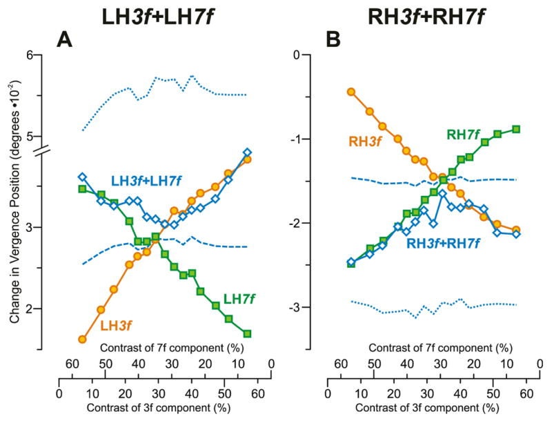
The initial vertical vergence responses to dual-grating stimuli with two disparities of the same sign: dependence on contrast (mean vergence position measures for subject BMS). (A): Responses when all stimuli had left-hyper disparity; green squares indicate data obtained with 7f stimuli (labeled LH7f); orange circles indicate data obtained with 3f stimuli (labeled LH3f); blue open diamonds indicate data obtained with 3f7f stimuli (labeled LH3f+LH7f); positive sign denotes left-sursumvergence. (B): Responses when all stimuli had right-hyper disparity; green squares indicate data obtained with 7f stimuli (labeled RH7f); orange circles indicate data obtained with 3f stimuli (labeled RH3f); blue open diamonds indicate data obtained with 3f7f stimuli (labeled RH3f+RH7f); negative sign denotes right-sursumvergence. Blue dotted lines, vector-sum predictions. Blue dashed lines, vector-average predictions. Note that the scales on the abscissas indicating the contrast of the 7f component are reversed. Data points are means of 113–120 samples, and SD’s ranged 0.006–0.011°.

More detailed analysis of these 3f7f data was problematic because the response measures were so restricted in range that noise was a serious factor despite the large number of responses used to obtain the averages. To improve the signal-to-noise ratio, response measures like those plotted in Fig. 10 were pooled by subtracting the mean response to each right-hyper stimulus from the mean response to the corresponding left-hyper stimulus. The resultant pooled measures for the data of subject BMS (based on the data in Fig. 10) are plotted in Fig. 11A and clearly retain the major features of the original measures, the 3f7f data (blue open diamonds) tracking the 3f data (orange circles) when the 3f component has the higher contrast and tracking the 7f data (green squares) when the 7f component has the higher contrast. These same features are also evident in the pooled response measures of the other two subjects (FAM, JRC): see Fig. 11B, C. The pooled response measures were also used to compute the Response Ratio of Sheliga et al. (2006b) defined by the following expression:

Fig. 11.

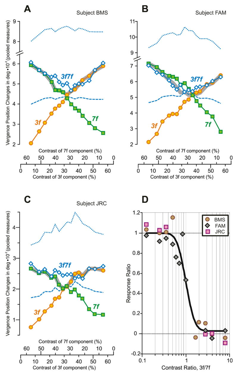
The initial vertical vergence responses to dual-grating stimuli with two disparities of the same sign: dependence on contrast and Contrast Ratio. (A–C): Dependence of pooled vergence position measures—obtained by subtracting the mean response to each right-hyper stimulus from the mean response to the corresponding left-hyper stimulus—on contrast for each of 3 subjects; orange circles, responses obtained with pure 3f stimuli; green squares, responses obtained with pure 7f stimuli; blue open diamonds, responses obtained with 3f7f stimuli; note that the scales on the abscissas indicating the contrast of the 7f component are reversed; thick grey line, Contrast-Weighted-Average model using Expression 2; blue dotted lines, vector-sum prediction; blue dashed lines, vector-average prediction. (A): subject BMS (n=113–120 response samples per stimulus; SD=0.006–0.011°). (B): subject FAM (n=197–208; SD=0.008–0.013°). (C): subject JRC (n=96–105; SD=0.005–0.009°). (D): Dependence of the Response Ratio on the Contrast Ratio (log scale), based on data in A–C from the 3 subjects (identified in the key); smooth black line is best-fit Cumulative Gaussian function.

$$\frac{R_{3f7f}-R_{3f}}{R_{7f}-R_{3f}}$$ (3)

where R_3f7f is the vergence response to the 3f7f stimulus when the 3f and 7f components have particular contrast values, and R_3f and R_7f are the vergence responses to pure 3f and 7f stimuli with matching contrast values. However, when R_3f and R_7f have very similar values so that the denominator of Expression 3 is very small, the Response Ratio is extremely sensitive to noise. For this reason, we discarded those Response Ratios whose denominators had a value <0.01° and then combined the remaining data from all three subjects into one plot: see Fig. 11D. Despite these strictures, the dependence of the Response Ratio on the Contrast Ratio in Fig. 11D clearly resembles those seen earlier in Fig. 4 and again is well fit by a Cumulative Gaussian (r²=0.960), with a SD of 0.16 log units, though the number of data points in the Transition Zone is small. The Transition Zone (based on the 5% and 95% criteria introduced earlier) extended from 0.59 to 1.93 so that, on average, a 1.8-fold difference in contrast was required for the one with the lower contrast to almost totally lose its influence (winner-take-all), which is comparable with that for the vertical 3f5f data.

4.2.2. Experiment 3b: horizontal vergence responses to horizontal disparities

The data obtained when horizontal disparities were applied to vertical 3f7f gratings were in all essentials like those just described when vertical disparities were applied to horizontal 3f7f gratings, except for showing greater trial-by-trial response variability. The general format of the Results is the same as for Experiment 3a. Figure 12 shows the change-in-vergence-position measures of subject FAM and is organized like Fig. 10, except that the data in Fig. 12A were obtained with crossed disparities and the data in Fig. 12B were obtained with uncrossed disparities. Despite the increased noise in the measures plotted in Fig. 12 it is nonetheless clear that, again, the 3f7f data (blue open diamonds) essentially tracked the data obtained with the pure 7f stimuli (green squares) when the 7f component had high contrast and tracked the data obtained with the pure 3f stimuli (orange circles) when the 3f component had high contrast. The responses to the dual-grating stimuli predicted by the vector average of the responses to the corresponding 3f and 7f stimuli again bisect the data obtained with the pure single-grating stimuli (blue dashed lines in Fig. 12) and the vector-sum predictions are again well outside the range of any recorded data (blue dotted lines in Fig. 12). Response measures like those plotted in Fig. 12 were again pooled—this time by subtracting the mean response to each uncrossed stimulus from the mean response to the corresponding crossed stimulus—and these pooled measures are shown for all three subjects in Fig. 13A–C, which is organized exactly like Fig. 11 and includes a plot of the Response Ratio versus the Contrast Ratio (Fig. 13D) based on the data for all three subjects exactly as in Fig. 11D. (For Fig. 13D we discarded those Response Ratios whose denominators had a value <0.01°.) Despite the greater noise in the horizontal vergence data, it is apparent that the plots in Fig. 13 are generally similar to those in Fig. 11, the 3f7f data converging on the 3f data when the 3f component has the higher contrast and on the 7f data when the 7f component has the higher contrast. Unfortunately, no transition data are available to constrain the best-fit Cumulative Gaussian in Fig. 13D (r²=0.96) so that we were not able to use this function to estimate the width of the Transition Zone. Nonetheless, it is clear that the transition is quite abrupt, with Response Ratios near unity having a Contrast Ratio as high as 0.7 and Response Ratios near zero having a Contrast Ratio as low as to 1.41.

Fig. 12.

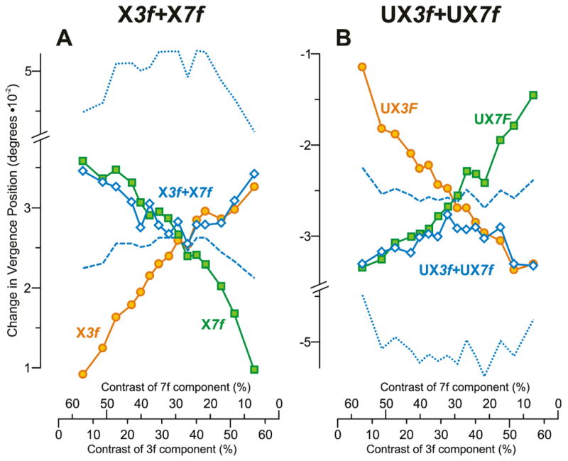
The initial horizontal vergence responses to dual-grating stimuli with two disparities of the same sign: dependence on contrast (mean vergence position measures for subject FAM). (A): Responses when all stimuli had crossed disparity; green squares indicate data obtained with 7f stimuli (labeled X7f); orange circles indicate data obtained with 3f stimuli (labeled X3f); blue open diamonds indicate data obtained with 3f7f stimuli (labeled X3f+X7f); positive sign denotes convergence. (B): Responses when all stimuli had uncrossed disparity; green squares indicate data obtained with 7f stimuli (labeled UX7f); orange circles indicate data obtained with 3f stimuli (labeled UX3f); blue open diamonds indicate data obtained with 3f7f stimuli (labeled UX3f+UX7f); negative sign denotes divergence. Blue dotted lines, vector-sum predictions. Blue dashed lines, vector-average predictions. Note that the scales on the abscissas indicating the contrast of the 7f component are reversed. Data points are means of 247–258 samples, and SD’s ranged 0.012–0.018°.

Fig. 13.

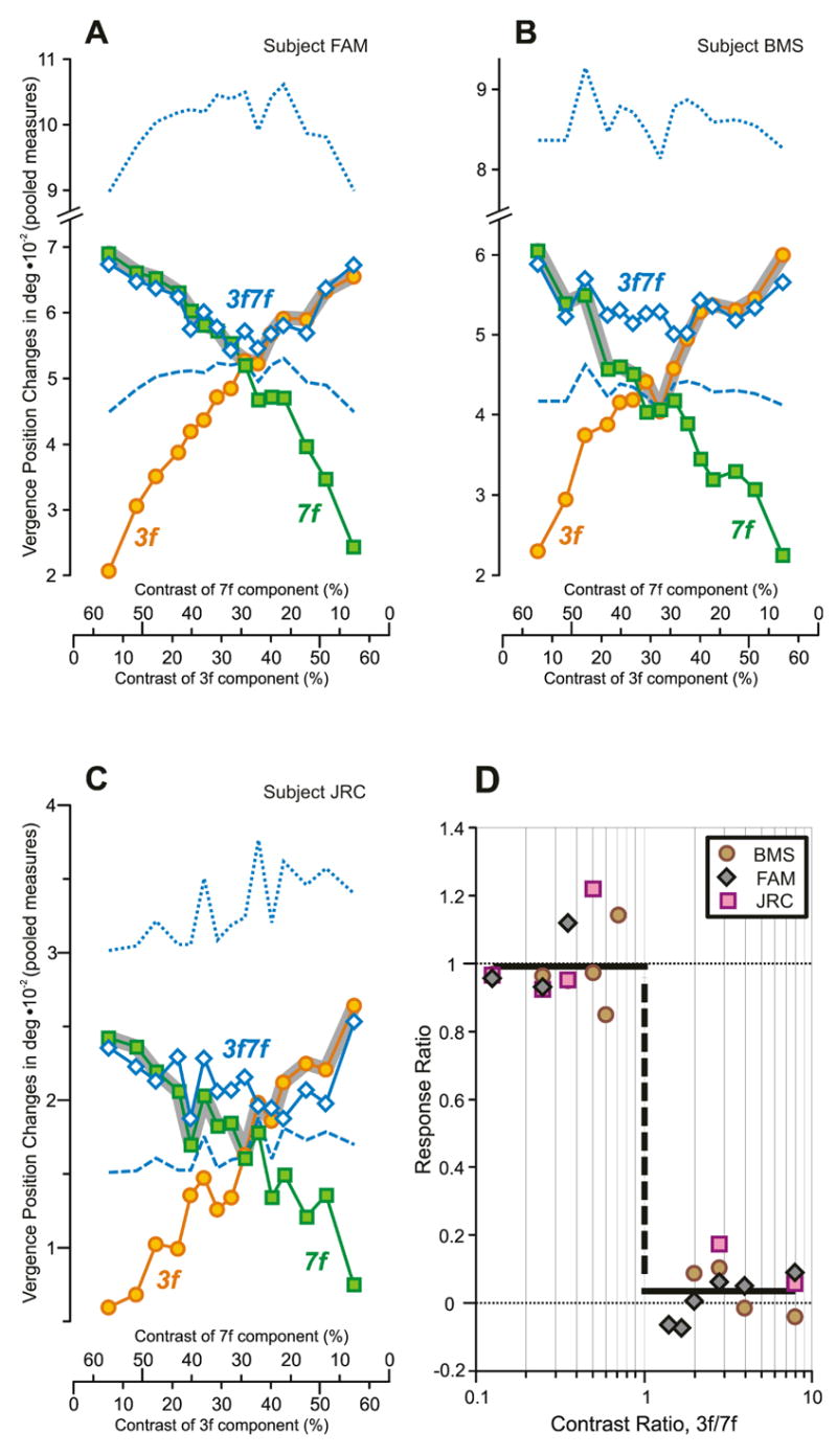
The initial horizontal vergence responses to dual-grating stimuli with two disparities of the same sign: dependence on contrast and Contrast Ratio. (A–C): Dependence of pooled vergence position measures—obtained by subtracting the mean response to each uncrossed stimulus from the mean response to the corresponding crossed stimulus—on contrast for each of 3 subjects; orange circles, responses obtained with pure 3f stimuli; green squares, responses obtained with pure 7f stimuli; blue open diamonds, responses obtained with 3f7f stimuli; note that the scales on the abscissas indicating the contrast of the 7f component are reversed; thick grey line, Contrast-Weighted-Average model using Expression 2; blue dotted lines, vector-sum prediction; blue dashed lines, vector-average prediction. (A): subject FAM (n=247–258 response samples per stimulus; SD=0.012–0.018°). (B): subject BMS (n=149–155; SD=0.015–0.029°). (C): subject JRC (n=106–117; SD=0.009–0.015°). (D): Dependence of the Response Ratio on the Contrast Ratio (log scale), based on data in A–C, from the 3 subjects (identified in the key); smooth black line is best-fit Cumulative Gaussian function (transition unconstrained).

4.3. Discussion of Experiment 3

The data in Figs. 10–13 indicate that when two superimposed sine waves have binocular disparities of the same sign but different magnitude (in our experiments, because they differ in spatial frequency) the resulting DVR depends critically on the relative contrasts of those two sine waves, and this dependence is highly nonlinear, involving an abrupt transition from dominance by one sine wave to dominance by the other: winner-take-all. Unfortunately, very few data are available in the transition itself, limiting our ability to define its abruptness. However, it is nonetheless evident from the plots in Figs. 11D and 13D that the transitions in the 3f7f data are at least as abrupt as those observed in the 3f5f data in Figs. 4 and 8 when the two disparities were of opposite sign.

The Contrast-Weighted-Average model generally provides a good fit to the 3f7f data in Fig. 11A–C and Fig. 13A–C only when the Contrast Ratio is less than ~0.5 or more than ~2: see the thick grey lines. Actually, in this “winner-take-all” region—Contrast Ratios ≥2 or ≤0.5—the Contrast-Weighted-Average model accounted for 87%, 74%, and 71% of variability in the vertical vergence data for subjects BMS, FAM, and JRC, respectively; for the horizontal vergence data these values were 50%, 89%, and 64% (though for subject BMS we here used Contrast Ratios <0.5 and >2). For Contrast Ratios between 0.5 and 2 the responses to 3f7f stimuli were consistently greater than those predicted by the Contrast-Weighted-Average model implying a partial summation of the two components.

Once more we invoke mutual inhibition to explain the nonlinear interactions between the neural mechanisms sensing the two disparities. However, whereas the disparities of the two harmonic components of the 3f5f stimulus might be distinguished on the basis of the signs and/or magnitudes of their two disparities and/or the spatial frequencies of the two sine waves, only the last two features are available to make this distinction with the 3f7f stimulus.

5. Closing remarks

5.1. Comparison of vertical and horizontal disparity vergence

There is accumulating evidence which suggests that the vertical vergence response is a rapid, purely involuntary reflex response to vertical disparity energy and functions solely to maintain the vertical alignment of the two eyes by eliminating vertical disparity errors, whereas the horizontal vergence response has both a rapid involuntary reflex component for eliminating small horizontal vergence errors and a slower, voluntary component that functions to transfer binocular fixation between objects in different depth planes (Busettini et al., 2001; Erkelens & Collewijn, 1985a; 1985b; 1991; Sheliga et al., 2005b; 2006a; Stevenson, 2002; Stevenson, Lott & Yang, 1997). Horizontal vergence also differs from vertical vergence in being responsive to a variety of non-disparity (monocular) depth cues—such as accommodation (see Judge, 1996, for review), radial optic flow (Busettini, Masson & Miles, 1997; Yang, Fitzgibbon & Miles, 1999), and complex attributes like perspective, overlay, size, relative motion, and perceived depth (e.g., Enright, 1987a; Enright, 1987b; Ringach, Hawken & Shapley, 1996; Sheliga & Miles, 2003)—as well as contrast-defined (i.e., pure 2^nd-order) disparities (Stevenson, 2002) and in being subject to attentional modulation (Stevenson et al., 1997). In the present study, however, we are concerned solely with the initial vergence responses that are elicited at short-latency when binocular disparities are applied to large-field stimuli. Though extremely small and necessitating the most sensitive methods to record them, these initial vergence responses provide a powerful new tool for studying the early neural processing of disparity. The reported differences between these reflex-like initial horizontal and vertical vergence responses in the literature have been quantitative rather than qualitative (Busettini et al., 2001; 1996; Sheliga et al., 2006a; Yang et al., 2003), and the findings in the present study are consistent with that: the nonlinear interactions were evident for both horizontal and vertical responses but were clearly stronger and more consistent across subjects for the vertical responses.

5.2. Winner-take-all: a nonlinearity favoring images in the plane of fixation?

The DVR is one of three kinds of ocular responses that can be elicited at ultra-short latency by large-field visual stimuli, the other two being the OFR, which generates version eye movements in response to motion in the plane of fixation (Gellman et al., 1990; Masson, Busettini, Yang & Miles, 2001; Miles et al., 1986), and the radial-flow vergence response (RFVR), which generates vergence eye movements in response to radial optic flow (Busettini et al., 1997; Yang et al., 1999). There is strong evidence that all are mediated by the medial superior temporal area of the cortex (Takemura et al., 2002a) and have a number of properties in common: see Miles (1998) for review of the earlier work, and Sheliga et al (2005a; 2006a; 2006b) for reviews of more recent work. As pointed out earlier, the current study was undertaken only after we had recorded the OFRs to two competing motions and found a nonlinear dependence on their relative contrasts (Sheliga et al., 2006b). The OFR is also known to be sensitive to horizontal disparity, which renders it insensitive to motion outside the plane of fixation (Masson et al., 2001), and it was argued that this would help the moving observer who looks off to one side to stabilize the images in the plane of fixation and ignore the competing image motions that occur in other depth planes because of motion parallax. It is known that the initial vergence responses to disparities applied to large-field stimuli also have a strong preference for objects in the immediate vicinity of the plane of fixation: the servo range for horizontal vergence only encompasses disparities of up to 2 or 3° (Busettini et al., 2001) and the vertical vergence mechanism responds best to vertical disparities when there is minimal horizontal disparity (Yang et al., 2003). We now suggest that the nonlinear interactions that work in favor of the images with the highest contrast will aid this process: because of accommodation, the retinal images of objects in the plane of fixation will tend to be better focused—and hence tend to have higher contrasts—than those of objects in other depth planes. In this scheme, the nonlinear interactions facilitate the selective engagement of the OFR and the DVR by objects in the plane of fixation and occur in the sensory—rather than the motor—pathways. The latter is consistent with the fact that the Contrast-Weighted-Average model—but not the Response-Weighted-Average model—provided a good fit to all of the 3f5f data.

References

- Adelson EH. Some new motion illusions, and some old ones, analysed in terms of their Fourier components. Investigative Ophthalmology and Visual Science. 1982;34(Suppl):144. (Abstract) [Google Scholar]
- Albrecht DG. Visual cortex neurons in monkey and cat: effect of contrast on the spatial and temporal phase transfer functions. Visual Neuroscience. 1995;12:1191–1210. doi: 10.1017/s0952523800006817. [DOI] [PubMed] [Google Scholar]
- Albrecht DG, Geisler WS, Frazor RA, Crane AM. Visual cortex neurons of monkeys and cats: temporal dynamics of the contrast response function. Journal of Neurophysiology. 2002;88:888–913. doi: 10.1152/jn.2002.88.2.888. [DOI] [PubMed] [Google Scholar]
- Brainard DH. The Psychophysics Toolbox. Spatial Vision. 1997;10:433–436. [PubMed] [Google Scholar]
- Busettini C, Fitzgibbon EJ, Miles FA. Short-latency disparity vergence in humans. Journal of Neurophysiology. 2001;85:1129–1152. doi: 10.1152/jn.2001.85.3.1129. [DOI] [PubMed] [Google Scholar]
- Busettini C, Masson GS, Miles FA. Radial optic flow induces vergence eye movements with ultra-short latencies. Nature. 1997;390:512–515. doi: 10.1038/37359. [DOI] [PubMed] [Google Scholar]
- Busettini C, Miles FA, Krauzlis RJ. Short-latency disparity vergence responses and their dependence on a prior saccadic eye movement. Journal of Neurophysiology. 1996;75:1392–1410. doi: 10.1152/jn.1996.75.4.1392. [DOI] [PubMed] [Google Scholar]
- Carandini M, Heeger DJ. Summation and division by neurons in primate visual cortex. Science. 1994;264:1333–1336. doi: 10.1126/science.8191289. [DOI] [PubMed] [Google Scholar]
- Carandini M, Heeger DJ, Movshon JA. Linearity and normalization in simple cells of the macaque primary visual cortex. The Journal of Neuroscience. 1997;17:8621–8644. doi: 10.1523/JNEUROSCI.17-21-08621.1997. [DOI] [PMC free article] [PubMed] [Google Scholar]
- Cogan AI, Kontsevich LL, Lomakin AJ, Halpern DL, Blake R. Binocular disparity processing with opposite-contrast stimuli. Perception. 1995;24:33–47. doi: 10.1068/p240033. [DOI] [PubMed] [Google Scholar]
- Cogan AI, Lomakin AJ, Rossi AF. Depth in anticorrelated stereograms: effects of spatial density and interocular delay. Vision Research. 1993;33:1959–1975. doi: 10.1016/0042-6989(93)90021-n. [DOI] [PubMed] [Google Scholar]
- Collewijn H, Van Der Mark F, Jansen TC. Precise recording of human eye movements. Vision Research. 1975;15:447–450. doi: 10.1016/0042-6989(75)90098-x. [DOI] [PubMed] [Google Scholar]
- Cormack LK, Stevenson SB, Schor CM. Disparity-tuned channels of the human visual system. Visual Neuroscience. 1993;10:585–596. doi: 10.1017/s0952523800005290. [DOI] [PubMed] [Google Scholar]
- Cumming BG, Parker AJ. Responses of primary visual cortical neurons to binocular disparity without depth perception. Nature. 1997;389:280–283. doi: 10.1038/38487. [DOI] [PubMed] [Google Scholar]
- Enright JT. Art and the oculomotor system: perspective illustrations evoke vergence changes. Perception. 1987a;16:731–746. doi: 10.1068/p160731. [DOI] [PubMed] [Google Scholar]
- Enright JT. Perspective vergence: oculomotor responses to line drawings. Vision Research. 1987b;27:1513–1526. doi: 10.1016/0042-6989(87)90160-x. [DOI] [PubMed] [Google Scholar]
- Erkelens CJ, Collewijn H. Eye movements and stereopsis during dichoptic viewing of moving random-dot stereograms. Vision Research. 1985a;25:1689–1700. doi: 10.1016/0042-6989(85)90141-5. [DOI] [PubMed] [Google Scholar]
- Erkelens CJ, Collewijn H. Motion perception during dichoptic viewing of moving random-dot stereograms. Vision Research. 1985b;25:583–588. doi: 10.1016/0042-6989(85)90164-6. [DOI] [PubMed] [Google Scholar]
- Erkelens CJ, Collewijn H. Control of vergence: gating among disparity inputs by voluntary target selection. Experimental Brain Research. 1991;87:671–678. doi: 10.1007/BF00227093. [DOI] [PubMed] [Google Scholar]
- Ferrera VP. Task-dependent modulation of the sensorimotor transformation for smooth pursuit eye movements. Journal of Neurophysiology. 2000;84:2725–2738. doi: 10.1152/jn.2000.84.6.2725. [DOI] [PubMed] [Google Scholar]
- Ferrera VP, Lisberger SG. Attention and target selection for smooth pursuit eye movements. The Journal of Neuroscience. 1995;15:7472–7484. doi: 10.1523/JNEUROSCI.15-11-07472.1995. [DOI] [PMC free article] [PubMed] [Google Scholar]
- Ferrera VP, Lisberger SG. The effect of a moving distractor on the initiation of smooth-pursuit eye movements. Visual Neuroscience. 1997;14:323–338. doi: 10.1017/s0952523800011457. [DOI] [PubMed] [Google Scholar]
- Fleet DJ, Wagner H, Heeger DJ. Neural encoding of binocular disparity: energy models, position shifts and phase shifts. Vision Research. 1996;36:1839–1857. doi: 10.1016/0042-6989(95)00313-4. [DOI] [PubMed] [Google Scholar]
- Gawne TJ, Kjaer TW, Richmond BJ. Latency: another potential code for feature binding in striate cortex. Journal of Neurophysiology. 1996;76:1356–1360. doi: 10.1152/jn.1996.76.2.1356. [DOI] [PubMed] [Google Scholar]
- Gellman RS, Carl JR, Miles FA. Short latency ocular-following responses in man. Visual Neuroscience. 1990;5:107–122. doi: 10.1017/s0952523800000158. [DOI] [PubMed] [Google Scholar]
- Hays AV, Richmond BJ, Optican LM. A UNIX-based multiple process system for real-time data acquisition and control. WESCON Conference Proceedings. 1982;2:1–10. [Google Scholar]
- Judge SJ. How is binocularity maintained during convergence and divergence? Eye. 1996;10(Pt 2):172–176. doi: 10.1038/eye.1996.43. [DOI] [PubMed] [Google Scholar]
- Krommenhoek KP, Wiegerinck WAJJ. A neural network study of precollicular saccadic averaging. Biological Cybernetics. 1998;78:465–477. doi: 10.1007/s004220050450. [DOI] [PubMed] [Google Scholar]
- Masson GS, Busettini C, Miles FA. Vergence eye movements in response to binocular disparity without depth perception. Nature. 1997;389:283–286. doi: 10.1038/38496. [DOI] [PubMed] [Google Scholar]
- Masson GS, Busettini C, Yang DS, Miles FA. Short-latency ocular following in humans: sensitivity to binocular disparity. Vision Research. 2001;41:3371–3387. doi: 10.1016/s0042-6989(01)00029-3. [DOI] [PubMed] [Google Scholar]
- Masson GS, Yang DS, Miles FA. Version and vergence eye movements in humans: open-loop dynamics determined by monocular rather than binocular image speed. Vision Research. 2002;42:2853–2867. doi: 10.1016/s0042-6989(02)00334-6. [DOI] [PMC free article] [PubMed] [Google Scholar]
- McGowan JW, Kowler E, Sharma A, Chubb C. Saccadic localization of random dot targets. Vision Research. 1998;38:895–909. doi: 10.1016/s0042-6989(97)00232-0. [DOI] [PubMed] [Google Scholar]
- Miles FA. The neural processing of 3-D visual information: evidence from eye movements. The European Journal of Neuroscience. 1998;10:811–822. doi: 10.1046/j.1460-9568.1998.00112.x. [DOI] [PubMed] [Google Scholar]
- Miles FA, Kawano K, Optican LM. Short-latency ocular following responses of monkey. I. Dependence on temporospatial properties of visual input. Journal of Neurophysiology. 1986;56:1321–1354. doi: 10.1152/jn.1986.56.5.1321. [DOI] [PubMed] [Google Scholar]
- Ohzawa I, DeAngelis GC, Freeman RD. Stereoscopic depth discrimination in the visual cortex: neurons ideally suited as disparity detectors. Science. 1990;249:1037–1041. doi: 10.1126/science.2396096. [DOI] [PubMed] [Google Scholar]
- Parker AJ, Cumming BG. Cortical mechanisms of binocular stereoscopic vision. Progress in Brain Research. 2001;134:205–216. doi: 10.1016/s0079-6123(01)34015-3. [DOI] [PubMed] [Google Scholar]
- Pelli DG. The VideoToolbox software for visual psychophysics: transforming numbers into movies. Spatial Vision. 1997;10:437–442. [PubMed] [Google Scholar]
- Pelli DG, Zhang L. Accurate control of contrast on microcomputer displays. Vision Research. 1991;31:1337–1350. doi: 10.1016/0042-6989(91)90055-a. [DOI] [PubMed] [Google Scholar]
- Port NL, Wurtz RH. Sequential activity of simultaneously recorded neurons in the superior colliculus during curved saccades. Journal of Neurophysiology. 2003;90:1887–1903. doi: 10.1152/jn.01151.2002. [DOI] [PubMed] [Google Scholar]
- Qian N. Computing stereo disparity and motion with known binocular properties. Neural Computation. 1994;6:390–404. [Google Scholar]
- Read JC, Cumming BG. Testing quantitative models of binocular disparity selectivity in primary visual cortex. Journal of Neurophysiology. 2003;90:2795–2817. doi: 10.1152/jn.01110.2002. [DOI] [PMC free article] [PubMed] [Google Scholar]
- Read JC, Parker AJ, Cumming BG. A simple model accounts for the response of disparity-tuned V1 neurons to anticorrelated images. Visual Neuroscience. 2002;19:735–753. doi: 10.1017/s0952523802196052. [DOI] [PubMed] [Google Scholar]
- Recanzone GH, Wurtz RH. Shift in smooth pursuit initiation and MT and MST neuronal activity under different stimulus conditions. Journal of Neurophysiology. 1999;82:1710–1727. doi: 10.1152/jn.1999.82.4.1710. [DOI] [PubMed] [Google Scholar]
- Ringach DL, Hawken MJ, Shapley R. Binocular eye movements caused by the perception of three-dimensional structure from motion. Vision Research. 1996;36:1479–1492. doi: 10.1016/0042-6989(95)00285-5. [DOI] [PubMed] [Google Scholar]
- Robinson DA. A method of measuring eye movement using a scleral search coil in a magnetic field. Institute of Electronic and Electrical Engineers: Transactions in Biomedical Engineering, BME- 1963;10:137–145. doi: 10.1109/tbmel.1963.4322822. [DOI] [PubMed] [Google Scholar]
- Sheliga BM, Chen KJ, FitzGibbon EJ, Miles FA. Initial ocular following in humans: a response to first-order motion energy. Vision Research. 2005a;45:3307–3321. doi: 10.1016/j.visres.2005.03.011. [DOI] [PMC free article] [PubMed] [Google Scholar]
- Sheliga BM, Chen KJ, Fitzgibbon EJ, Miles FA. Short-latency disparity vergence in humans: evidence for early spatial filtering. Annals of the New York Academy of Sciences. 2005b;1039:252–259. doi: 10.1196/annals.1325.024. [DOI] [PMC free article] [PubMed] [Google Scholar]
- Sheliga BM, Fitzgibbon EJ, Miles FA. Short-latency disparity vergence eye movements: A response to disparity energy. Vision Research. 2006a;46:3723–3740. doi: 10.1016/j.visres.2006.04.020. [DOI] [PMC free article] [PubMed] [Google Scholar]
- Sheliga BM, Kodaka Y, FitzGibbon EJ, Miles FA. Human ocular following initiated by competing image motions: Evidence for a winner-take-all mechanism. Vision Research. 2006b;46:2041–2060. doi: 10.1016/j.visres.2005.11.033. [DOI] [PMC free article] [PubMed] [Google Scholar]
- Sheliga BM, Miles FA. Perception can influence the vergence responses associated with open-loop gaze shifts in 3D. Journal of Vision. 2003;3:654–676. doi: 10.1167/3.11.2. [DOI] [PMC free article] [PubMed] [Google Scholar]
- Stevenson SB. Visual processing in disparity vergence control. Annals of the New York Academy of Sciences. 2002;956:492–494. doi: 10.1111/j.1749-6632.2002.tb02864.x. [DOI] [PubMed] [Google Scholar]
- Stevenson SB, Cormack LK, Schor CM, Tyler CW. Disparity tuning in mechanisms of human stereopsis. Vision Research. 1992;32:1685–1694. doi: 10.1016/0042-6989(92)90161-b. [DOI] [PubMed] [Google Scholar]
- Stevenson SB, Lott LA, Yang J. The influence of subject instruction on horizontal and vertical vergence tracking. Vision Research. 1997;37:2891–2898. doi: 10.1016/s0042-6989(97)00109-0. [DOI] [PubMed] [Google Scholar]
- Takemura A, Inoue Y, Kawano K. Visually driven eye movements elicited at ultra-short latency are severely impaired by MST lesions. Annals of the New York Academy of Sciences. 2002a;956:456–459. doi: 10.1111/j.1749-6632.2002.tb02854.x. [DOI] [PubMed] [Google Scholar]
- Takemura A, Inoue Y, Kawano K, Quaia C, Miles FA. Single-unit activity in cortical area MST associated with disparity-vergence eye movements: evidence for population coding. Journal of Neurophysiology. 2001;85:2245–2266. doi: 10.1152/jn.2001.85.5.2245. [DOI] [PubMed] [Google Scholar]
- Takemura A, Kawano K, Quaia C, Miles FA. Population coding in cortical area MST. Annals of the New York Academy of Sciences. 2002b;956:284–296. doi: 10.1111/j.1749-6632.2002.tb02827.x. [DOI] [PubMed] [Google Scholar]
- Usui S, Amidror I. Digital low-pass differentiation for biological signal processing. IEEE Transactions on Biomedical Engineering. 1982;29:686–693. doi: 10.1109/TBME.1982.324861. [DOI] [PubMed] [Google Scholar]
- Yang D, Fitzgibbon EJ, Miles FA. Short-latency vergence eye movements induced by radial optic flow in humans: dependence on ambient vergence level. Journal of Neurophysiology. 1999;81:945–949. doi: 10.1152/jn.1999.81.2.945. [DOI] [PubMed] [Google Scholar]
- Yang DS, FitzGibbon EJ, Miles FA. Short-latency disparity-vergence eye movements in humans: sensitivity to simulated orthogonal tropias. Vision Research. 2003;43:431–443. doi: 10.1016/s0042-6989(02)00572-2. [DOI] [PMC free article] [PubMed] [Google Scholar]