

Abstract
This paper presents a probabilistic neural network based technique for unsupervised quantification and segmentation of brain tissues from magnetic resonance images. It is shown that this problem can be solved by distribution learning and relaxation labeling, resulting in an efficient method that may be particularly useful in quantifying and segmenting abnormal brain tissues where the number of tissue types is unknown and the distributions of tissue types heavily overlap. The new technique uses suitable statistical models for both the pixel and context images and formulates the problem in terms of model-histogram fitting and global consistency labeling. The quantification is achieved by probabilistic self-organizing mixtures and the segmentation by a probabilistic constraint relaxation network. The experimental results show the efficient and robust performance of the new algorithm and that it outperforms the conventional classification based approaches.
Index Terms: Finite mixture models, image segmentation, information theoretic criteria, model estimation, probabilistic neural networks, relaxation algorithm
I. Introduction
Quantitative analysis of brain tissues refers to the problem of estimating tissue quantities from a given image, and segmentation of the image into contiguous regions of interest to describe the anatomical structures. The problem has recently received much attention largely due to the improved fidelity and resolution of medical imaging systems. Because of its ability to deliver high resolution and contrast, magnetic resonance (MR) imaging has been the dominant modality for research on this problem [1]–[5]. In clinical practice, MR images are typically analyzed by qualitative, or semi-quantitative visualization and evaluation. The main focus of most automatic MR image analysis schemes has been on image segmentation [2], [4], [6]–[9]. Tissue quantification, on the other hand, alone or together with tissue segmentation, also provides valuable information for brain tissue analysis [1], [5]. Pathological studies show that many neurological diseases are accompanied by subtle changes in brain tissue quantities and volumes [3]. Because of the practical difficulty for clinicians to identify all pathological changes directly from medical images, development of accurate and efficient image analysis systems is of great importance.
Stochastic model-based methods have been by far the most popular approach for quantification of brain tissues from MR images [1], [3], [5], [10]–[12]. The stochastic model-based approach typically employs a finite mixture model that is shown to be a very suitable model for the task [1], [3], [10]. Neural networks have also been employed for image segmentation [2], [6], [7], [13], and recently, a cross fertilization of the stochastic model based and neural network approaches, probabilistic neural networks have emerged as a powerful tool in MR image analysis [7], [14]. Probabilistic neural networks provide valuable insight for designing and learning in neural networks and offer efficient online computation of the quantities of interest, a feature especially important for evaluation of studies in a clinical setting, such as MR image sequence analysis [12]. Furthermore, probabilistic neural networks are particularly suitable for application to quantitative analysis of MR images. In this paper, we present a probabilistic neural network approach for efficient analysis of brain tissues by using single-valued MR brain scans. The major differences of our work from the previous research described in [1], [3], [5], [9] are as follows.
We present two theorems to show that the correct use of the standard finite normal mixture (SFNM) model in MR brain tissue quantification does not require the pixel images to be statistically independent.
We introduce and briefly describe a new information theoretic criterion formulation following Jaynes’ principle: the minimum conditional bias and variance (MCBV) criterion. We use three information theoretic criteria to determine the appropriate number of tissue types in a particular MR brain scan.
We introduce an on-line algorithm for parameter estimation associated with tissue quantification: the probabilistic self-organizing mixtures (PSOM) algorithm. We present comparative results to show its superior performance in terms of faster rate of convergence and lower floor of estimation error and introduce global relative entropy (GRE) as the objective function for error measure.
We introduce an efficient procedure for pixel classification associated with tissue segmentation that is realized by a probabilistic constraint relaxation network (PCRN). PCRN might be considered as an extension of the inhomogeneous Markov random field based approaches [15].
Experimental results demonstrate the efficient and reliable performance of the proposed scheme, in terms of the quantification achieved by PSOM, consistent order determination using three information criteria including MCBV, and the satisfactory segmentation results by PCRN.
The paper is organized as follows. In Section II, we present the stochastic modeling formulation, for both the tissue quantification and the segmentation stages. We present the algorithms to solve these problems in Section in along with results using simulated data. Section IV presents examples, with real MR data. These results demonstrate the accuracy and reproducibility of the method and show the performance of efficient automatic quantification and segmentation. We present discussion of the results in Section V.
II. Problem Statement
In this section, we present the problem formulation and the probabilistic network models used for tissue quantification and segmentation.
A. Stochastic Modeling
In order to validate the use of a suitable stochastic model for MR image analysis with a specified objective, we have studied MR imaging statistics and observed several useful statistical properties of MR images [16], [19]. These results are strongly supported by the analysis of actual MR image data [20]. In particular, based on the statistical properties of MR pixel images, where pixel image is defined as the observed gray level associated with the pixel, use of an SFNM distribution is justified to model the image histogram, and it is shown that the SFNM model converges to the true distribution when the pixel images are asymptotically independent [21]. Furthermore, by incorporating statistical properties of context images, where context image is defined as the membership of the pixel associated with different tissue types, a localized SFNM formulation is proposed to impose local consistency constraints on context images in terms of a stochastic regularization scheme [16].
Assume that each pixel in the MR image can be decomposed into pixel image x and context image l. By ignoring information regarding the spatial ordering of pixels, we can treat context images (i.e., pixel labels) as random variables and describe them using a multinomial distribution with unknown parameters πk, k = 1 ···, K. Since it reflects the distribution of the total number of pixels in each tissue type (or component), πk can be interpreted as a prior probability of pixel labels determined by the global context information. Thus, the relevant (sufficient) statistics are the pixel image statistics for each component and the number of pixels of each component. The marginal probability measure for any pixel image, i.e., the SFNM distribution, can be obtained by writing the joint probability density of x and l and then summing the joint density over all possible outcomes of l, i.e., fr(x) = Σl f(x, l), resulting in a sum of the following general form according to the Bayes law:
| (1) |
with , and
where μk and are the mean and variance of the kth Gaussian kernel. We use K to denote the number of Gaussian components and to denote the total parameter vector that includes μk, , and πk for all K components. Several observations are worth reiterating.
All pixel images are identically distributed from a maximum-entropy mixture distribution and treated as unclassified data [22]–[24].
The SFNM model uses the prior probabilities of pixel label in the formulation instead of realizing its true value for each pixel image.
Since the calculation of the histogram of pixel images relies on the same mechanism as SFNM modeling, it can be considered to be a sampled version of the true pixel distribution [1].
Since the structure of the likelihood function in SFNM model follows an identical distribution [25], the corresponding ML estimation will be unbiased [26]. However, the price to be paid for the stationary structure is that we cannot represent local context explicitly, i.e., the pixel labels are hidden. Because context information is of particular importance in tissue segmentation, by assuming that the context images are random variables with Markovian property [15], a localized SFNM model is formulated. It explicitly incorporates local context regularities into a consistent network structure. For each pixel i, we define the spatial constraint as a local set of all pairs (li,lj) such that the consistency between li and lj can be represented by the indicator function I(li, lj) [2], [13], [27]. Under this configuration, all pairs of labels are either compatible (produce an output “1”) or incompatible (produce an output “0”) [28]. We define the neighborhood of pixel i denoted by δi, by opening a b × b window with pixel i being the central pixel, where b is assumed to be an odd integer. Similar to the approach taken in [2], [4], and [13], we compute the frequency of neighbors of pixel i with labels compatible to a given label k, conditioning the labels of its neighbors by
| (2) |
and the localized SFNM distribution for xi directly follows by
| (3) |
The calculation of πik is same with that of πk, however, its scale is local and thus can be interpreted as the conditional prior of the pixel label determined by the uncertainty contained in lδi. The localized SFNM model hence provides a more evident meaning than the SFNM model for tissue segmentation [15], while the SFNM model has a better structure for tissue quantification [23].
B. Tissue Quantification
Tissue quantification addresses the combined estimation of tissue parameters and the detection of the tissue structural parameter K in (1) given the pixel images x. The two main approaches used to determine these parameters are classification-based estimation and distance minimization approaches [25], [29]. In the classification-based approach, all pixels are first classified into different components according to a specified distance measure, and then, the model parameters are estimated using sample averages by the ergodic theorems [6], [9], [29]. In the distance minimization approach, the mixture density is fitted to the histogram of pixel images by finding the optimal parameters with respect to a distance measure [1], [3], [21]. We use relative entropy (the Kullback-Leibler distance) [26] for tissue quantification in MR images such that it measures the information theoretic distance between the histogram of the pixel images, denoted by fx, and the estimated SFNM distribution fr(x), and is given by [26]
| (4) |
Note that the use of the relative entropy cost also overcomes problems such as convergence at the wrong extreme faced by the squared error cost function as it weighs errors more heavily when probabilities are near zero and one, and diverges in the case of convergence at the wrong extreme [17], [30]. We have shown that, when relative entropy is used as the distance measure, distance minimization is equivalent to maximum likelihood (ML) estimation of SFNM parameters. The conclusion is summarized by the following theorem [38].
Theorem 1
Consider a sequence of random variables x1, ···,xN in Assume that the sequence {xi} is independent and identically distributed (i.i.d.) by the distribution fr. Then, the joint likelihood function is determined only by the histogram of data and is given by
| (5) |
where H denotes the entropy with base e [26]. Hence, maximization of joint likelihood function is equivalent to the minimization of relative entropy D(fx||fr).
Thus, tissue quantification is formulated as a distribution learning problem and quantification is achieved when the relative entropy (4) is minimized, or by Theorem 1, when the joint likelihood function is maximized. However, spatial statistical dependence among pixel images is one of the fundamental issues in problem formulation since the calculation of the image histogram treats all pixel images as independent random variables [1], [5]. In order to validate the correct use of (4) in tissue quantification, we prove the following theorem in [38] to show that the image histogram fx converges to the true distribution f* with probability one as N → ∞.
Theorem 2
Consider a sequence of random variables x1, ···,xN in . Assume that the sequence {xi}is asymptotically independent [26] and identically distributed by the SFNM distribution f*. For a closed convex set and distribution fx ∉ E, let fr ∈ E be the distribution that achieves the minimum distance to fx, i.e.,
| (6) |
Then, when N approaches infinity, we have
| (7) |
with probability one, i.e., the estimated distribution of x, fr, given that it achieves the minimum of D(fx||fr), is close to f* for large N.
Thus, when N is sufficiently large, minimization of the relative entropy between fr and f* can be well approximated by the minimization of the relative entropy between fr and fx. This fitting procedure can be practically implemented by maximizing the joint likelihood function under the independence approximation of pixel images [18].
C. Tissue Segmentation
Anatomical structure, in addition to the results of tissue quantification that reveals different tissue properties, provides very valuable information in medical applications. Tissue segmentation is a technique for partitioning the image into meaningful regions corresponding to different objects. It may be considered as a clustering process where the pixels are classified into attributed tissue types according to their gray-level values and spatial correlation [6]. A reasonable assumption that can be made is that spatially close pixels are likely to belong to the same tissue type [22]. Accordingly, tissue segmentation addresses the realization of context images li, i = 1, ···, N, given the observed pixel images x. Based on the localized SFNM model (3), a deterministic relaxation labeling can be used to update the context images after global tissue quantification. With a motivation similar to the one in [2] and [6], the technique seeks for a consistent labeling solution where the criterion is to maximize global consistency measure by using a system of inequalities. The structure of relaxation labeling is motivated by two basic considerations: i) decomposition of a global computation scheme into a network performing simple local computations, and ii) use of suitable local context regularities in resolving ambiguities.
We can define the consistency of discrete relaxation labeling and formalize its relationship to global optimization as follows: We first define the component in the localized SFNM distribution (3) as a support function consisting of the compatibility function ∧(li,lδi) and local likelihood p(xi|li):
| (8) |
Note that the support function Si(k) is a function of the component (tissue type) k. Then, tissue segmentation is interpreted as the satisfaction of a system of inequalities as follows:
| (9) |
for all k and for i = 1,···, N, where a consistent labeling is defined as the one having maximum support at each pixel simultaneously. We further define the average local consistency measure
| (10) |
to link consistent labeling to global optimization [28]. It is shown that when the spatial compatibility measure is symmetric and A(l) attains a local maximum at l, then l is a consistent labeling [2], [8], [13], [28]. Hence, a consistent labeling can be accomplished by locally maximizing A(l).
We can view consistency as a “locking-in” property, i.e., since the support function defined for a given pixel depends on the current labels of neighboring pixels, this neighborhood influences the update of the given pixel through probabilistic compatibility constraints. With constraint propagation, the relaxation process iteratively updates the label assignments to increase the consistency, and ideally finds a more consistent labeling with the neighboring labels, such that each pixel is designated a unique label [2], [16].
III. Theory and Algorithms
Over the years, several unsupervised approaches have been reported in the literature exploring quantitative analysis of MR brain images [1], [5]. Currently, there are two main approaches to the problem. In the first one, the maximum likelihood quantification scheme, tissue types are first quantified using maximum likelihood principle, where only soft classification of the pixel images is required [1]. Further classification of a sample is then performed by placing it into the class for which the posterior probability or the support function is maximum, i.e., by Bayesian consistent labeling [45], [46]. The quantities obtained by sample averages after imperfect pixel classification may not be consistent with the previous quantification result [23]. In the second approach, tissue quantification and segmentation are performed simultaneously with back and forth iterations between the two. In this case, the prior and post quantification results will be consistent, however the quantification and classification errors do interfere with each other during the iterations. In this research, we deal with tissue quantification and segmentation as two separate objectives and use different optimality criteria. However, it is worth reiterating the fact that the proposed method achieves an unbiased ML tissue quantification, a step to be considered independent from the following tissue segmentation step. In what follows, we present the theory and algorithms for the two stages: i) quantification that involves network order selection and adaptive computation of the parameters to achieve soft classification, and ii) segmentation that uses the order and the parameters computed in the quantification stage to perform hard classification by incorporating local context constraints.
A. Adaptive Model Selection
Since the prior knowledge of the true structure of a real image is generally not available, it is most often desirable to have a neural network structure that is adaptive, in the sense that the number of local components (i.e., hidden nodes) is not fixed beforehand. Both for PSOM and PCRN, using a smaller or larger number of mixture components (local components in the network) than the number of tissue types actually represented on a particular slice will result in incorrect identification and quantification of the tissues in a particular slice. This situation is particularly critical in a real clinical application where the structure of the individual slice for a particular patient may be arbitrarily complex. The objective of adaptive model selection is to propose a systematic strategy for the determination of the structure of the network, i.e., the number of hidden nodes (or mixture components) K in the two probabilistic neural networks: the PSOM and the PCRN. One approach to determine the optimal number K0 is to use information theoretic criteria, such as the Akaike information criterion (AIC) [31], [32], and the minimum description length (MDL) [5], [33]. The major thrust of this approach has been the formulation of a structural learning in which a model fitting procedure is utilized to select a model from several competing candidates such that the selected model best fits the observed data.
For example, AIC will select the model that gives the minimum of
| (11) |
where is the likelihood of r̂ML, the ML parameter estimates, and Ka is the number of free adjustable parameters in the model. The AIC tries to formulate the problem explicitly as a problem of approximation of the true structure by the model. It implies that the correct number of distinctive image regions K0 can be obtained by minimizing AIC. From a quite different point of view, MDL reformulates the problem explicitly as an information coding problem in which the best model fit is measured such that high probabilities are assigned to the observed data while at the same time the model itself is not too complex to describe [33]. The model is selected by minimizing the total description length defined by
| (12) |
Note that, different from AIC, the second term in MDL takes into account the number of observations. However, the justifications for the optimality of these two criteria with respect to tissue quantification or classification are somewhat indirect and remain unresolved [5], [21], [25], [31].
In this section, we present a new formulation of information theoretic criterion, the minimum conditional bias and variance criterion, to address the model selection problem. Akaike and Rissanen’s work on information theoretic criteria have certainly been the inspirational source to this work, however, in our work, we present a new interpretation and justification by information theoretic means [18]. Our approach has a simple optimal appeal in that it selects a minimum conditional bias and variance model, i.e., if two models are about equally likely, MCBV selects the one whose parameters can be estimated with the smallest variance.
New formulation is based on the fundamental argument that the value of the structural parameter can not be arbitrary or infinite, because such an estimate might be said to have low “bias” but the price to be paid is high “variance” [34]. We can obtain a formulation by using Jaynes’ principle, which states that “the parameters in a model which determine the value of the maximum entropy should be assigned values which minimize the maximum entropy” [35]. Let joint entropy of x and r̂ be H(x, r̂) = H(x|r̂) + H(r̂). It is shown that the maximum of conditional entropy H(x|r̂) is precisely the negative of the logarithm of the likelihood function corresponding to the entropy-maximizing distribution for x [33]. We have
| (13) |
where uniform randomization in the SFNM modeling corresponds to the maximum uncertainty [22], [23]. Furthermore, maximizing the entropy of the parameter estimates H(r̂) results in
| (14) |
where we have used the result that, given the variance of parameter estimate determined by the corresponding sample average, the normal and independent distribution Pr̂. gives the maximum entropy [24], [26], [36].
Since the joint maximum entropy is a function of Ka and r̂, by taking the advantage of the fact that model estimation is separable in components and structure, we define the MCBV criterion as
| (15) |
where is the conditional bias (a form of information theoretic distance) [24], [26], and is the conditional variance (a measure of model uncertainty) [24], [36], of the model. As both of these two terms represent natural estimation errors about the true models, we treat them on an equal basis. A minimization of the expression in (15) leads to the following characterization of the optimum estimation:
| (16) |
That is, if the cost of model variance is defined as the entropy of parameter estimates, the cost of adding new parameters to the model must be balanced by the reduction they permit in the ideal code length for the reconstruction error. A practical MCBV formulation with code-length expression is further given by [18], [26]
| (17) |
where the calculation of H(r̂KML) requires the estimation of the true ML model parameter values. It is shown that, for sufficiently large number of observations, the accuracy of the ML estimation tends quickly to the best possible accuracy determined by the Cramér-Rao lower bounds (CRLB’s) [36]. Thus, the CRLB’s of the parameter estimates are used in the actual calculation to represent the “conditional” bias and variance [37]. We have found that, experimentally, the MCBV formulation for determining the value of K0 exhibits very good performance consistent with both the AIC and the MDL criteria. It should be noted, however, that it is not the only plausible one; other criteria such as cross validation techniques may also be useful in this case [46], [48], [50], [52], [53].
We present a simulation study to test the performance of model selection with the proposed criterion (MCBV) and the two frequently used methods, AIC and MDL. We generate a test data with four overlapping normal components. Each component represents one local cluster. The value for each component is set to a constant value and normally distributed noise is then added to this simulation phantom with a signal-to-noise ratio (SNR) of 10 dB [38]. The phantom is shown in Fig. 1(a). The AIC, MDL, and MCBV curves, as functions of the number of local clusters K, are plotted in the same figure, Fig. 1(b). According to the information theoretic criteria, the minima of these curves indicate the correct number of the image components. From this experimental figure, it is clear that the number of local clusters suggested by these criteria are all correct. More application of the MCBV to the identification of real data structures will be presented in Section IV.
Fig. 1.

Experimental results of model selection, algorithm initialization, and final quantification on the simulated image, (a) Original image with four components, (b) Curves of the AIC/MDL/MCBV criteria where the minimum corresponds to K0 = 4. (c) Initial histogram learning by the ALMHQ algorithm, (d) Final histogram learning by the PSOM algorithm.
B. Probabilistic Self-Organizing Mixtures
There are many numerical techniques to perform the ML estimation of finite mixture distributions [25]. The most popular method is the expectation-maximization (EM) algorithm [44]. EM algorithm first calculates the posterior Bayesian probabilities of the data through the observations and the current parameter estimates (E-step) and then updates parameter estimates using generalized mean ergodic theorems (M-step). The procedure cycles back and forth between these two steps. The successive iterations increase the likelihood of the model parameters. A neural network interpretation of this procedure is given in [39]. However, EM algorithm has the reputation of being slow, since it has a first order convergence in which new information acquired in the expectation step is not used immediately [40]. Recently, on-line versions of the EM algorithm are proposed for large scale sequential learning. Such a procedure obviates the need to store all the incoming observations, changes the parameters immediately after each data point allowing for high data rates. Titterington [25] has developed a stochastic approximation procedure which is closely related to our approach, and shows that the solution can be made consistent. Other similar formulations are due to Marroquin et al. [29] and Weinstein et al. [41].
The PSOM we present here is a fully unsupervised and incremental stochastic learning algorithm, and is a generalized adaptive structure version of the SOFM algorithm we presented in [21]. The scheme provides winner-takes-in probability (Bayesian “soft”) splits of the data, hence allowing the data to contribute simultaneously to multiple tissues. By differentiating D(fx||fr) given in (4) with respect to the unconstrained parameters, μk and , we obtain the following standard gradient descent learning rule for the mean and variance parameter vectors:
| (18) |
| (19) |
where λ is the learning rate and is the posterior Bayesian probability, defined by
| (20) |
By adopting a stochastic gradient descent scheme for minimizing D(fx||fr) [29], the corresponding on-line formulation is obtained by simply dropping the summation in (18) and (19) which results in
| (21) |
| (22) |
where the variance factors are incorporated into the learning rates while the posterior Bayesian probabilities are kept, and a(t) and b(t) are introduced as the learning rates, two sequences converging to zero, ensuring unbiased estimates after convergence. This modified version of the parameter updates is motivated by the principle that assigning different learning rates to different parameters of a network and allowing those to vary over time increases the rate of convergence [42]. Based on generalized mean ergodic theorem [26], updates can also be obtained for the constrained regularization parameters, πk, in the SFNM model. For simplicity, given an asymptotically convergent sequence, the corresponding mean ergodic theorem, i.e., the recursive version of the sample mean calculation, should hold asymptotically. Thus, we define the interim estimate of πk [43] by
| (23) |
Hence, the updates given by (21)–(23) provide the incremental procedure for computing the SFNM component parameters. Their practical use however requires strongly mixing condition and a decaying annealing procedure (learning rate decay) [26], [27], [36]. These two steps are currently controlled by user-defined parameters which may not be optimized for a specific problem. In addition, algorithm initialization must be chosen carefully and appropriately. In [43], we introduce an adaptive Lloyd-Max histogram quantization (ALMHQ) algorithm for threshold selection which is also well suited to initialization in ML estimation. In this work, we employ ALMHQ for initializing the network parameters μk, , and πk.
We tested the proposed technique using the same simulated image shown in Fig. 1(a). After the algorithm initialization by ALMHQ [43], network parameters are finalized by the PSOM algorithm. The GRE value is used as an objective measure to evaluate the accuracy of quantification. The results of the distribution learning are shown in Fig. 1(c) and (d). The GRE in the initial stage achieves a value of 0.0399 nats, and after the final quantification by PSOM, is down to 0.008 nats. The numerical results are given in Table I where the unit of μ and σ2 simply represents the observed gray levels of the pixel images while π is the probability measure. To simplify the representation, we omit their units as in [1], [5].
TABLE I.
True Parameter Values and the Estimates for the Simulated Image of Fig. 1
| True | Initial | Final | ||||||||||
|---|---|---|---|---|---|---|---|---|---|---|---|---|
| k | 1 | 2 | 3 | 4 | 1 | 2 | 3 | 4 | 1 | 2 | 3 | 1 |
| π | 0.25 | 0.125 | 0.5 | 0.125 | 0.234 | 0.234 | 0.364 | 0.185 | 0.23 | 0.135 | 0.48 | 0.157 |
| μ | 86 | 126 | 166 | 206 | 81 | 131 | 167 | 205 | 84 | 121 | 164 | 201 |
| σ2 | 400 | 400 | 100 | 100 | 235 | 158 | 157 | 177 | 354 | 365 | 373 | 463 |
We also present a comparison of the performance of PSOM with that of the EM [23], [40], [44] and the competitive learning (CL) [29] algorithms in MR brain tissue quantification (see Section IV). We evaluate the computational accuracy and efficiency of the algorithm in standard finite normal mixture (SFNM) distribution learning, based on an objective criterion and its learning curve characteristics. For comparison, we applied all methods to the same example and used the GRE value between the image histogram and the estimated SFNM distribution as the goodness criterion to evaluate the quantification error. Fig. 2(a) shows learning curves of the PSOM and competitive learning (CL) algorithms, averaged over five independent runs. As observed in the figure, PSOM outperforms CL learning by faster convergence and lower quantification error, and reaches a final GRE value of about 0.04 nats. Fig. 2(b) presents the comparison of the performance of the PSOM algorithm with that of the EM algorithm for 25 epochs. As seen in the learning curves, PSOM algorithm again shows superior estimation performance. Note that since the EM algorithm uses intrinsically a batch learning mode, the learning curve appears very smooth when each point on the curve corresponds to a completed learning cycle in this case. The final quantification error is about 0.02 nats for PSOM with a faster convergence rate.
Fig. 2.

Comparison of the learning curves of PSOM and CL (left) and EM (right).
To conclude the discussion on PSOM, we address two issues regarding the nature of PSOM as it relates to neural computation. These are, the adjustment of structures in the feature space by the algorithm and the temporal dynamics of the learning process at the single neuron and the modular levels. Mapping the self-organizing operation to the PSOM, we design a network where both the structure and weights are updated according to an unsupervised learning procedure. Information theoretic criteria are shown to provide a reasonable approach for the solution of the problem. Another issue relating to the neural computational aspect of the PSOM procedure is the temporal dynamics of the learning process. As given by (21)–(23), learning in PSOM is a dynamic feedback competitive learning procedure in a self-organizing map (SOM) [27]. In particular, both the structure and the weights of the PSOM “compete” for the assignment order of each model and assignment probability of each observation. Overall convergence dynamics of the PSOM are similar to SOM in that a solution is obtained by “resonating” between input data and an internal representation. Such a mechanism can be considered as a more realistic learning than the batch EM procedure. In addition, temporal dynamics of the learning process for PSOM on the structure level, suggest the adjustment of the internal structure of a neural network as more information is acquired, i.e., the addition of new clusters.
C. Probabilistic Constraint Relaxation Networks
Given the SFNM parameters, i.e., the image components computed by the ML principle, there are several approaches to perform pixel classification. When the true pixel labels are considered to be functionally independent and nonrandom constants, competitive learning approaches can be used for the segmentation of different tissue types [6], [8]. ML classification directly maximizes the individual likelihood function of pixel images by placing pixel i into the Kth region, if
| (24) |
where the term in parentheses is the modified Mahalanobis distance. On the other hand, when pixel labels are considered to be random variables, and the global context is taken as the prior information, probabilistic neural networks are most commonly used for tissue segmentation [4], [7]. By minimizing the expected value of the total Bayes classification error, pixel i will be classified into the Kth region if
| (25) |
where the term in parentheses, since it incorporates the global prior information πk, is called the Bayesian distance.
The major problem with these approaches is that the classification error will be high when the observed images are noisy, and possibly, there will be a high bias in the model parameters computed with sample averages after classification. We propose a probabilistic constraint relaxation network (PCRN) to perform tissue segmentation by imposing neighborhood context regularities to alleviate the two problems mentioned above. It operates on an initial segmented image, preferably one with uniformly distributed classification errors, such as the one segmented by the classification-maximization (CM) algorithm [29]. PCRN uses stochastic discrete gradient descent procedure where each pixel is randomly visited and its label is updated [16], [45], i.e., pixel i is classified into the kth region if
| (26) |
where πik is defined in (2) and the decision follows a probabilistic compatibility constraint given by
As discussed in Section II-C, by employing local maximization, relaxation labeling searches for a consistent labeling such that the average total consistency measure given by (10) is maximized for the given support function (8) [2]. It has been shown that relaxation labeling based on the stochastic discrete gradient descent principle converges to a steady point such that no label needs to be updated and the solution corresponds to at least one local maximum of A(l) (10), [2], [16], [28], [29]. Iterations are needed to search for a consistent labeling, i.e., to maximize (10) for the given support function (8). During this relaxation process, our numerical experiments show that classification error decreases at every iteration and converges to a local maximum. Although a complete consistent labeling may not be reached in a practical implementation, the relaxation labeling algorithm, can provide a quite reasonable and accurate segmentation usually within few iterations [28]. The procedure can be summarized as follows.
PCRN Algorithm
Given l(0), m = 0
randomly visit each pixel for i = 1, …, N (by random permutation of pixel ordering), and update its label li according to (26);
when the percentage of label changing less that ∈%, stop. Otherwise, m = m + 1 and repeat step 2.
As mentioned before, it is desirable to start with an initial labeling l(0) which has classification errors that have spatial uniform distribution on the initial segmented image. Our experience has shown ML classification described by (24) to be a very good candidate to perform the initialization, i.e., to compute l(0) since it results in uniformly distributed classification errors. Also, a reasonable stopping criterion, suggested by our experimental results is 1%, i.e., choosing ∈ = 1 in step 2.
As shown in Fig. 3(a), PCRN is composed of an N dimensional input array (the pixel images), a K dimensional hidden layer, and an N dimensional output array of pixel labels, such that each takes a value li = k, where k = 1, …, K. The number of the hidden units K, corresponding to the number of tissue types, is determined by information theoretic criteria as explained in Section II-A during tissue quantification. The estimates of the model parameters also determine the parameters μk and for each of the K units . Each of these K hidden units combines the local probabilistic constraint with the global intensity distribution information to produce an output which competes with the outputs of other hidden units to produce the labeling for the ith pixel, i.e., to determine the output li. The incorporation of the local context information is achieved by a gating function between the hidden units and the output, realizing πik given in (2), providing feedback from the output units to determine the activation of the hidden unit. Hence, the network, rather than minimizing an energy function as in [6], [8], [29], looks for a possible local maximum of a global consistency measure by operating on local probabilistic constraints. It is derived directly from probabilistic constraints and can be classified as a recurrent noncausal competitive network with gating functions that incorporate context constraints. This approach demonstrates how a network of discrete units can be used to search an optimal solution to a problem that benefits the incorporation of context constraints.
Fig. 3.
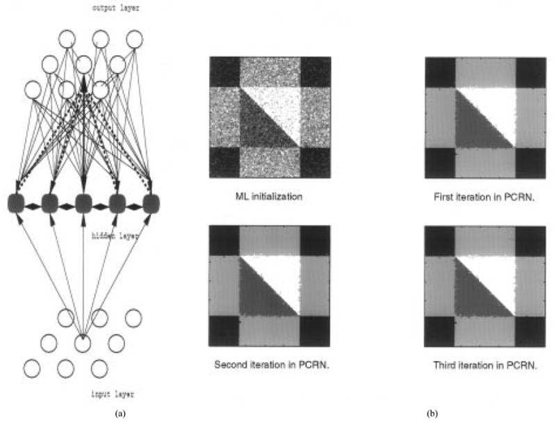
(a) PCRN structure, (b) Image segmentation by PCRN on simulated image (with initialization by ML classification).
Given the configuration of PCRN that is partially determined in model selection and estimation, the input layer of the PCRN has neurons corresponding to each pixel image and the output layer has neurons each corresponding to the labels of the original image. Competition within hidden layer ensures that only one neuron becomes active at any pixel location. This is accomplished by a winner-takes-all scheme among neurons, i.e., by a competitive learning procedure [29]. Gating between output and the hidden layer incorporates the local labeling information to provide locally consistent labeling and hence to remove the ambiguities. This is performed by the use of consistent measures between neighborhood neurons. Reciprocal feedback from output to gating unit allows each hidden neuron to control its activation. Another important difference between the PCRN and the conventional competitive learning network is that the recurrent gating provides a mechanism to incorporate the local Bayesian prior in the decision-making process through a consistency constraint. Without a similar mechanism, the conventional methods can only achieve, at best, a ML or a global Bayesian classification.
For validation of image segmentation using PCRN, we apply the algorithm first to the simulated images shown in Fig. 1(a). We use ML classifier to initialize the image segmentation, i.e., to initialize the quantified image by selecting the pixel label with the largest likelihood at each node by (24). Our experience suggested this to be a very suitable starting point for relaxation labeling [16]. PCRN is then used to fine tune the image segmentation. Since the true scene is known in this experiment, the percentage of total classification error is used as the criterion for evaluating the performance of the segmentation technique. In Fig. 3(b), the initial segmentation by the ML classification and the step-wise results of three iterations in PCRN are presented. In this experiment, algorithm initialization results in an average misclassification of 30%. It can be clearly seen that a dramatic improvement is obtained after several iterations of the PCRN by using local constraints determined by the context information. Also, note that the convergence is fast, as after the first iteration, most misclassifications are removed. The final percentage of classification errors for Fig. 3 is about 0.7935%.
IV. Experiments and Results
In this section, we present results from real MR brain images using the probabilistic neural network based approach we introduced to quantify and segment tissue types. In Section III, after introducing the algorithms, we presented results using a simulated tone image for which the number and structure of regions were known beforehand. The results presented showed the success of the scheme in determining the correct number of regions and the reliable definition of the boundaries of regions. In this section, we concentrate on application of the method to real MR images, which presents a great challenge to any computerized unsupervised analysis technique because of its complex structure. Furthermore, in addition to the assessment of radiologists, we also introduce application of an objective measure, GRE, to assess the performance of the scheme after quantification and segmentation, i.e., the soft and hard classification stages.
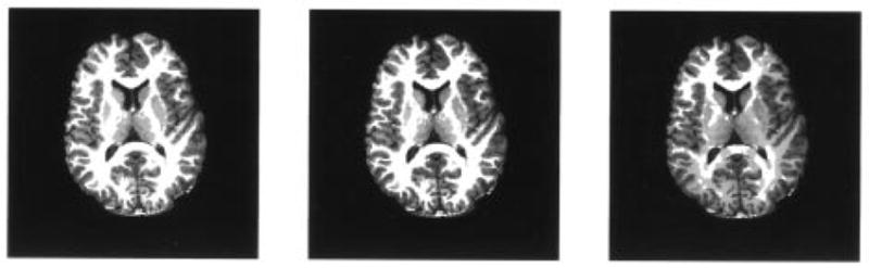
Fig. 4 shows the original data consisting of three adjacent, T1-weighted images parallel to the AC-PC line. The data are acquired with a GE Sigma 1.5 Tesla system. The imaging parameters are TR 35, TE 5, flip angle 45°, 1.5 mm effective slice thickness, 0 gap, 124 slices with in-plane 192 × 256 matrix, and 24 cm field of view. Since the skull, scalp, and fat in the original brain images do not contribute to the brain tissue, we edit the MR images to exclude nonbrain structures prior to tissue quantification and segmentation as explained in [16]. This also helps us to achieve better quantification and segmentation of brain tissues by delineation of other tissue types that are not clinically significant [1], [2], [5]. The extracted brain tissues are shown in Fig. 5. For each slice in the test sequence, the corresponding histograms are given in Fig. 6. As seen in the figure, the histogram has a considerably different characteristics from slice to slice and the tissue types are all highly overlapping making the problem quite complex. Our main objective is to assess the accuracy and repeatability of the results obtained with the method on real MR images. Evaluation of different image analysis techniques is a particularly difficult task, and dependability of evaluations by simple mathematical measures such as squared error performance is questionable. Therefore, most of the time, the quality assessment of the quantified and segmented image usually depends heavily on the subjective and qualitative judgements. As mentioned before, in this work, besides the evaluation performed by radiologists, we use the GRE value to reflect the quality of tissue quantification and also present results using EM and CL for image quantification to compare the results of our scheme in terms of both the accuracy and the efficiency of the procedure. For assessment of tissue segmentation, we use post-segmentation sample averages as an indirect but objective criterion, and again use GRE values and visual inspection.
Fig. 4.
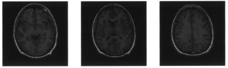
Test sequence of MR image brain scans (original images).
Fig. 5.

Pure brain tissues extracted from original images.
Fig. 6.

Histograms of the brain tissue images.
Based on the pre-edited MR brain image, the procedure for analysis of tissue types in a slice is summarized as follows.
For each value of K (number of tissue types), K = Kmin, ···, Kmax, ML tissue quantification is performed by the PSOM algorithm [(20)–(23)].
Scan the values of K = Kmin, ···, Kmax, use MCBV (16) to determine the suitable number of tissue types.
Select the result of tissue quantification corresponding to the value of K0 determined in step 2.
Initialize tissue segmentation by ML classification (23).
Finalize tissue segmentation by PCRN (by implementing (25) as explained in Section III-C).
The performance of tissue quantification and segmentation is then evaluated in terms of the GRE value, convergence rate, computational complexity, and visual judgement.
As discussed in the literature, the brain is generally composed of three principal tissue types, i.e., white matter (WM), gray matter (GM), cerebrospinal fluid (CSF), and their pair-wise combinations, called the partial volume effect. Santago and Gage [1] have proposed a six-tissue model representing the primary tissue types and the mixture tissue types which were defined as CSF-White (CW), CSF-Gray (CG), and Gray-White (GW). In this work, we also consider the triple mixture tissue, defined as CSF-White-Gray (CWG). More importantly, since the MR image scans clearly show the distinctive intensities at local brain areas, the functional areas within a tissue type need to be considered. In particular, the caudate nucleus and putamen are two important local brain functional areas. In our experiment, as we have noted before, we allow the number of tissue types to vary from slice to slice, i.e., consider adaptability to different MR images. We let Kmin = 2 and Kmax = 9 and calculate AIC(K) (11), MDL(K) (12), and MCBV(K) (15) for K = Kmin, ···, Kmax. The results with these three criteria are shown in Fig. 7, which suggest that the brain images contain six, eight, and six tissue types, respectively. According to the model fitting procedure using information theoretic criteria as explained before, the minima of these criteria indicate the most appropriate number of the tissue types, which is also the number of hidden nodes in the corresponding PSOM (mixture components in SFNM). In the calculation of MCBV using (16), we used the CRLB’s to represent the conditional variances of the parameter estimates, given by [37]
Fig. 7.

Results of model selection for slice 1–3 (K0 = 6, 8, 6, left to right).
| (27) |
| (28) |
| (29) |
Note that since the true parameter values in above equations are not available, their ML estimates are used to obtain the approximate CRLB’s. From Fig. 7, it is clear that, with real MR brain images, the overall performance of the three information theoretic criteria is fairly consistent. Our experience suggests that, however, AIC tends to overestimate while MDL tends to underestimate the number of tissue types [38], and MCBV provides a solution between those of AIC and MDL, which we believe to be more reasonable especially in terms of providing a balance between the bias and variance of the parameter estimates.
When performing the computation of the information theoretic criteria, we used PSOM to iteratively quantify different tissue types for each fixed K. The PSOM algorithm is initialized by a fully automatic thresholding technique, i.e., the adaptive ALMHQ procedure that we have introduced in [43]. For slice 2, the results of final tissue quantification with K0 = 7, 8, 9 are shown in Fig. 8. Table II gives the numerical result of final tissue quantification for slice 2 corresponding to K0 = 8, where a GRE value of 0.02–0.04 nats is achieved. It was found that most of the variance parameters are different, which suggests that assuming same variance for each tissue type with distinct image-intensity distribution is not very realistic. These quantified tissue types agree with those of physician’s qualitative analysis results [54], [55].
Fig. 8.

Histogram learning for slice 2 (K = 7, 8, 9 from top to bottom).
TABLE II.
Result of Parameter Estimation for Slice 2
| tissue type | 1 | 2 | 3 | 4 | 5 | 6 | 7 | 8 |
|---|---|---|---|---|---|---|---|---|
| π | 0.0251 | 0.0373 | 0.0512 | 0.071 | 0.1046 | 0.1257 | 0.2098 | 0.3752 |
| μ | 38.848 | 58.718 | 74.400 | 88.500 | 97.864 | 105.706 | 116.642 | 140.294 |
| σ2 | 78.5747 | 42.282 | 56.5608 | 34.362 | 24.1167 | 23.8848 | 49.7323 | 96.7227 |
The PCRN tissue segmentation for slice 2 is performed with K0 = 7, 8, 9, and the algorithm is initialized by ML classification [see (24)]. PCRN updates are terminated after five to ten iterations, since further iterations produced almost identical results. The segmentation results are shown in Fig. 9. Although the segmentation result contains some small isolated spots (less than four-pixel size), the PCRN approach is quite encouraging. It is seen that the boundaries of WM, GM, and CSF are delineated very well and successfully. To see the benefit of using information theoretic criteria in determining the number of tissue types, the decomposed tissue type segments are given in Fig. 10 with K0 = 8. As can be observed in Figs. 9 and 10, the segmentation with eight tissue types provides a very meaningful result. The regions with different gray levels are satisfactorily segmented, especially, the major brain tissues are clearly identified. If the number of tissue types were “underestimated” by one, tissue mixtures located within putamen and caudate areas would be lumped into one component, though the results are still meaningful. When the number of tissue type was “overestimated” by one, there is no significant difference in the quantification result, but white matter has been divided into two components. For K0 = 8, the segmented regions represent eight types of brain tissues: (a) CSF, (b) CG, (c) CGW, (d) GW, (e) GM, (f) putamen area, (g) caudate area, and (h) WM as shown in Fig. 10. These segmented tissue types also agree with the results of radiologists’ evaluation [54], [55].
Fig. 9.
Results of tissue segmentation for slice 2 with k0 = 7,8,9 (from left to right).
Fig. 10.

Result of tissue type decomposition for slice 2 which represent eight types of brain tissues: CSF, CG, CGW, GW, GM, putamen area, caudate area, and WM (left to right, top to bottom).
We then test the hypotheses that: i) tissue segmentation using the prior constraint that the MR image has a locally piecewise continuous structure provides better results than those of using global regularization together with local intensity values [called global Bayesian classification (GBC)]; and ii) tissue quantification using soft classification (i.e., without realizing the value of li, by ML quantification) is more accurate than the quantification results obtained by using sample averages computed after hard pixel classification, (i.e., by a winner-takes-all scheme), or than those obtained in conjunction with such a scheme. For this task, slice 2 is segmented and postquantified, using the Bayesian approach [i.e., global Bayesian classification based on (25)] and the sample averages. The global Bayesian approach is not iterative and does not require a stopping point. In this work, the performance is evaluated by the post-GRE values for all schemes, which is consistent with model-based ergodic principle and allows for uniform comparison among various techniques. Table III gives the classification errors by these two methods in terms of postquantification errors. It can be seen that quantification by PSOM results in lower error than GBC and PCRN, with PCRN resulting in lower GRE value. This result implies that the intrinsic misclassification in tissue segmentation creates a biased parameter estimate that contributes to the higher quantification error, as also noted in [23]. It is very interesting to note that, since ergodic theorem is the most fundamental one behind any statistical model-based image analysis approach, postquantification may be a suitable objective criterion for evaluating the quality of image segmentation in a fully unsupervised situation.
TABLE III.
Comparison of Segmentation Error Resulting from Noncontextual and Contextual Methods for Slice 2
| Method | PSOM | GBC | PCRN |
|---|---|---|---|
| (soft) | (hard-GBC) | (hard-PCRN) | |
| GRE value (nats) | 0.0067 | 0.4406 | 0.1578 |
V. Discussions and Conclusions
We have presented a complete procedure for quantifying and segmenting major brain tissue types from MR images, in which two kinds of probabilistic neural networks: soft and hard classifiers, are employed. The MR brain image is modeled by a standard finite normal mixture model and an extended localized formulation. Information theoretic criteria are applied to detect the number of tissue types thus allowing the corresponding network to adapt its structure for the best representation of the data. The PSOM algorithm is used to quantify the parameters of tissue types leading to a ML estimation. Segmentation of identified tissue components is then implemented by PCRN through Bayesian decision. The results obtained by using the simulated image and real MR brain images demonstrate the promise and effectiveness of the proposed technique. In particular, the number of tissue types and the associated parameters were consistently estimated. The tissue types were satisfactorily segmented. Although the current algorithms were tested for 2-D images, their application to 3-D situations is straightforward by appropriate neighborhood function in PCRN.
Our main contribution is the complete proposal of a three-step learning strategy for determination of both the modular structure and the components of the network. In this approach, the network structure (in terms of suitability of the statistical model) is justified in the first step. It is followed by soft segmentation of data such that each data point supports all local components simultaneously. The associated probabilistic labels are then realized in the third step by competitive learning of this induced hard classification task.
We introduced a model selection scheme that explicitly incorporates the bias and variance dilemma in finite data training. When tested with synthetic and actual data, the results show that the number of hidden nodes in PSOM should be adjusted to match the data, and hence order selection may be important to consider. Theory is developed showing that ML quantification and Bayesian classification have distinct objectives, and both soft and hard classification problems are studied which describe performance differences. The quantification results from the presegmentation and the postsegmentation stages generated the evidence. However, the results of tissue segmentation that includes probabilistic constraints, indicate that the use of local context information can provide better results that is often consistent with the recurrent network structure.
The main limitations of the current approach are that i) it requires the testing of all possible network structure candidates during the model fitting procedure, hence is not efficient especially for processing MR sequence images where an online learning might be preferred, and ii) applications to real MR data indicates the possibility of being trapped in a local maximum in ML estimation by the PSOM since there is no guarantee of attaining the global maximum.
There are possible ways to mitigate these problems: Since one possible contribution to the local minima problem is imperfect initialization, we use a simple automated threshold selection, based on Lloyd-Max histogram quantization [43], to systematically initialize the algorithm during model selection and quantification. Experimental results suggested that the method is quite effective in a variety of situations with different data structures [16], [21], [43]. To address the first limitation mentioned above, we tested an adaptive model selection procedure by incorporating the correlation between slices in a given MR sequence. More precisely, model selection starts from a slice in the middle of the sequence and moves in each direction, such that for slice i + 1, we set and where is the optimal number of tissue types for slice i given by the information theoretic criteria. It should be addressed, however, that they are by no means the only, or the best, possible solutions; in fact, it will be interesting to compare the effect of random and systematic algorithm initialization on the final performance, and further study is needed for interpretation of the results of these information theoretic criteria: AIC, MDL, and MCBV.
To summarize, the results of the experiments we have performed indicate the plausibility of our approach for brain tissue analysis from MRI scans, and show that it can be applied to clinical problems such as those encountered in tissue segmentation and quantitative diagnosis.
Acknowledgments
The authors would like to thank T. Lei of the University of Maryland, Baltimore, S. K. Mun and M. T. Freedman of the Georgetown University Medical Center, and R. F. Wagner of the U.S. Food and Drug Administration, for their valuable input and guidance on this work.
This work was supported in part by the Office of Naval Research under Grant N00014-94-1-0743 and by the U.S. Army Medical Research and Material Command under DAMD 18-97-I-2078 DAR.
Biographies
Yue Wang (S’93–M’95) received the B.S. and M.S. degrees from Shanghai Jiao Tong University, Shanghai, China, in 1984 and 1987, respectively, and the Ph.D. degree from University of Maryland-Baltimore County, in 1995, all in electrical engineering.
During 1995–1996, he was a Post-doctoral Fellow at the Georgetown University Medical Center, Washington, DC. In 1996, he joined the Department of Electrical Engineering and Computer Science, Catholic University of America, Washington, DC, as an Assistant Professor. He is also affiliated with the Department of Radiology, Georgetown University School of Medicine, as an Adjunct Assistant Professor. He is the Guest Editor for the Journal of Intelligent Automation and Soft Computing. He is currently on the National Cancer Institute working group on lung cancer imaging. His research interests include image analysis, medical imaging, information visualization, data base mapping, volumetric display, visual explanation, and their applications in biomedicine and multimedia informatics.
Dr. Wang is the recipient of a 1998 U.S. Army Medical Research and Material Command CDA Award.

Tülay Adalý (S’88–M’92) received the B.S. degree from Middle East Technical University, Ankara, Turkey, in 1987 and the M.S. and Ph.D. degrees from North Carolina State University, Raleigh, in 1988 and 1992, respectively, all in electrical engineering.
In 1992, she joined the Department of Electrical Engineering, University of Maryland-Baltimore County, as an Assistant Professor. Her research interests are in neural computation, adaptive signal processing, estimation theory, and their applications in channel equalization, biomedical image analysis, soliton communications, and time-series prediction. She has authored or co-authored more than 75 publications.
Dr. Adalý is the Guest Editor of a special issue of the Journal of VLSI Signal Processing Systems for Signal, Image, and Video Technology on Neural Networks on neural networks for biomedical image processing. She currently serves on the IEEE Technical Committee on Neural Networks for Signal Processing and the IEEE Signal Processing Conference Board. She is the recipient of a 1997 National Science Foundation CAREER Award.
Sun-Yuan Rung (S’74–M’78–SM’84–F’88), for a photograph and biography, see this issue, p. 1095.
Zsolt Szabo received the M.D. degree from the University of Belgrade and the Ph.D. degree from the University of Dusseldorf. He received postgraduate training at the University of Dusseldorf, Germany, and the Johns Hopkins Medical Institutions, Baltimore, MD, and special training in positron emission tomography (PET) at the Nuclear Research Center, Julich, Germany.
He is an Associate Professor of Radiology at the Johns Hopkins Medical Institutions. His research activities involve PET/MRI coregistration, partial volume correction, investigation of serotonin and dopamine transporters and investigation of angiotensin II receptors with PET. His special interests include nuclear medicine and PET with special emphasis on receptor imaging and neuroscience.
Dr. Szabo is member of the Society of Nuclear Medicine and of the German Association of Nuclear Medicine.

Contributor Information
Yue Wang, Y. Wang is with the Department of Electrical Engineering and Computer Science, The Catholic University of America, Washington, DC 20064 USA, and is affiliated with the Department of Radiology, Georgetown University School of Medicine, Washington, DC 20007 USA (e-mail: wang@pluto.ee.cua.edu)..
Tülay Adalý, T. Adali is with the Department of Computer Science and Electrical Engineering, University of Maryland-Baltimore County, Baltimore, MD 21250 USA (e-mail: adali@engr.umbc.edu)..
Sun-Yuan Kung, S.-Y. Kung is with the Department of Electrical Engineering, Princeton University, Princeton, NJ 08544 USA (e-mail: kung@ee.princeton.edu)..
Zsolt Szabo, Z. Szabo is with the Department of Radiology, Johns Hopkins Medical Institutions, Baltimore, MD 21205 USA (e-mail: zszabo@welchlink.welch.jhu.edu)..
References
- 1.Santago P, Gage HD. Quantification of MR brain images by mixture density and partial volume modeling. IEEE Trans Med Imag. 1993 Sept;12:566–574. doi: 10.1109/42.241885. [DOI] [PubMed] [Google Scholar]
- 2.Worth AJ, Kennedy DN. Segmentation of magnetic resonance brain images using analog constraint satisfaction neural networks. In: Barrett HH, Gmitro AF, editors. Information Processing in Medical Imaging. Berlin, Germany: Springer-Verlag; 1993. pp. 225–243. [Google Scholar]
- 3.Choi HS, Haynor DR, Kim Y. Partial volume tissue classification of multichannel magnetic resonance images—A mixture model. IEEE Trans Med Imag. 1994 Sept;10:395–407. doi: 10.1109/42.97590. [DOI] [PubMed] [Google Scholar]
- 4.Cline HE, Lorensen WE, Kikinis R, Jolesz R. Three-dimensional segmentation of MR images of the head using probability and connectivity. J Comp Assist Tomog. 1990;14:1037–1045. doi: 10.1097/00004728-199011000-00041. [DOI] [PubMed] [Google Scholar]
- 5.Liang Z, MacFall JR, Harrington DP. Parameter estimation and tissue segmentation from multispectral MR images. IEEE Trans Med Imag. 1994 Sept;13:441–449. doi: 10.1109/42.310875. [DOI] [PubMed] [Google Scholar]
- 6.Cheng KS, Lin JS, Mao CW. The application of competitive Hopfield neural network to medical image segmentation. IEEE Trans Med Imag. 1996 Aug;15:560–567. doi: 10.1109/42.511759. [DOI] [PubMed] [Google Scholar]
- 7.Morrison M, Attikiouzel Y. Proc Conf Neural Networks. Vol. 3. Baltimore, MD: 1992. A probabilistic neural network based image segmentation network for magnetic resonance images; pp. 60–65. [Google Scholar]
- 8.Dhawan AP, Arata L. Segmentation of medical images through competitive learning. Comput Meth Prog Biomed. 1993;40:203–215. doi: 10.1016/0169-2607(93)90058-s. [DOI] [PubMed] [Google Scholar]
- 9.Hall LO, et al. A comparison of neural network and fuzzy clustering techniques in segmenting magnetic resonance images of the brain. IEEE Trans Neural Networks. 1992;3:672–682. doi: 10.1109/72.159057. [DOI] [PubMed] [Google Scholar]
- 10.Wang Y, Adalý T, Lau CM, Szabo Z. Quantification of MR brain images by a probabilistic self-organizing map. Radiology. 1995 Nov;197:252–253. [Google Scholar]
- 11.Wang Y, Adalý T, Lau CM, Kung SY. Quantitative analysis of MR brain image sequences by adaptive self-organizing finite mixtures. J VLSI Tech Signal Process. 1998;8:219–239. [Google Scholar]
- 12.Adalý T, Wang Y, Gupta N. A block-wise relaxation labeling scheme and its application to edge detection in cardiac MR image sequences. to be published. [Google Scholar]
- 13.Lin WC, Tsao ECK, Chen CT. Constraint satisfaction neural networks for image segmentation. Pattern Recognit. 1992;25:679–693. [Google Scholar]
- 14.Wang Y, Adalý T. Probabilistic neural networks for parameter quantification in medical image analysis. In: Vossoughi J, editor. Biomedical Engineering Recent Development. 1994. [Google Scholar]
- 15.Wang Y. PhD dissertation. Univ. Maryland; College Park, MD: May, 1995. MR Imaging statistics and model-based MR image analysis. [Google Scholar]
- 16.Wang Y, Adalý T, Freedman MT, Mun SK. MR brain image analysis by distribution learning and relaxation labeling. Proc. 15th South. Biomedical Engineering Conf; Dayton, OH. Mar. 1996; pp. 133–136. [Google Scholar]
- 17.Adalý T, Liu X, Sönmez MK. Conditional distribution learning with neural networks and its application to channel equalization. IEEE Trans Signal Processing. 1997 Apr;45:1051–1064. [Google Scholar]
- 18.Wang Y. Image quantification and the minimum conditional bias/variance criterion. Proc. 30th Conf. Information Science and Systems; Princeton, NJ. Mar. 20–22, 1996; pp. 1061–1064. [Google Scholar]
- 19.Wang Y, Lei T. A new stochastic model-based image segmentation technique for MR images. Proc. 1st IEEE Int. Conf. Image Processing; Austin, TX. 1994. pp. 182–185. [Google Scholar]
- 20.Fuderer M. The information content of MR images. IEEE Trans Med Imag. 1988;7:368–380. doi: 10.1109/42.14521. [DOI] [PubMed] [Google Scholar]
- 21.Wang Y, Adalý T. Efficient learning of finite normal mixtures for image quantification. Proc. IEEE Int. Conf. Acoustics, Speech, and Signal Processing; Atlanta, GA. 1996. pp. 3422–3425. [Google Scholar]
- 22.Bouman C, Liu B. Multiple resolution segmentation of texture images. IEEE Trans Pattern Anal Machine Intell. 1991 Feb;13:99–113. [Google Scholar]
- 23.Titterington DM. Comments on ‘application of the conditional population-mixture model to image segmentation’. IEEE Trans Pattern Anal Machine Intell. 1984 Sept;6:656–658. doi: 10.1109/tpami.1983.4767412. [DOI] [PubMed] [Google Scholar]
- 24.Rissanen J. System Identification, Advances and Case Studies. New York: Academic; 1976. Minimax entropy estimation of models for vector processes; pp. 97–119. [Google Scholar]
- 25.Titterington DM, Smith AFM, Markov UE. Statistical Analysis of Finite Mixture Distributions. New York: Wiley; 1985. [Google Scholar]
- 26.Cover TM, Thomas JA. Elements of Information Theory. Wiley; 1991. [Google Scholar]
- 27.Haykin S. Neural Networks: A Comprehensive Foundation. New York: Macmillan; 1994. [Google Scholar]
- 28.Hummel RA, Zucker SW. On the foundations of relaxation labeling processes. IEEE Trans Pattern Anal Machine Intell. 1983 May;5 doi: 10.1109/tpami.1983.4767390. [DOI] [PubMed] [Google Scholar]
- 29.Marroquin JL, Girosi F. Some extensions of the K-means algorithm for image segmentation and pattern classification. Tech. Rep., MIT Artif. Intell. Lab; Cambridge, MA. Jan. 1993. [Google Scholar]
- 30.Adalý T, Sönmez MK, Patel K. On the dynamics of the LRE Algorithm: A distribution learning approach to adaptive equalization. Proc. IEEE Int. Conf. Acoustics, Speech, Signal Processing; Detroit, MI. 1995. pp. 929–932. [Google Scholar]
- 31.Akaike H. A new look at the statistical model identification. IEEE Trans Automat Contr. 1974 Dec;19 [Google Scholar]
- 32.Zhang J, Modestino JM. A model-fitting approach to cluster validation with application to stochastic model-based image segmentation. IEEE Trans Pattern Anal Machine Intell. 1990 Oct;12:1009–1017. [Google Scholar]
- 33.Rissanen J. A universal prior for integers and estimation by minimum description length. Ann Stat. 1983;11 [Google Scholar]
- 34.Geman S, Bienenstock E, Doursat R. Neural networks and the bias/variance dilemma. Neural Comput. 1992;4:1–52. [Google Scholar]
- 35.Jaynes ET. Information theory and statistical mechanics. Phys Rev. 1957 May;108:620–630. 171–190. [Google Scholar]
- 36.Poor HV. An Introduction to Signal Detection and Estimation. Berlin, Germany: Springer-Verlag; 1988. [Google Scholar]
- 37.Perlovsky LI. Cramer-Rao Bounds for the estimation of normal mixtures. Pattern Recognit Lett. 1989;10:141–148. [Google Scholar]
- 38.Wang Y, Lin SH, Li H, Kung SY. Data mapping by probabilistic modular network and information theoretic criteria. IEEE Trans Signal Processing. 1998 to be published. [Google Scholar]
- 39.Perlovsky L, McManus M. Maximum likelihood neural networks for sensor fusion and adaptive classification. Neural Networks. 1991;4:89–102. [Google Scholar]
- 40.Xu L, Jordan MI. On convergence properties of the EM algorithm for Gaussian mixture. Tech. Rep., MIT Artif. Intell. Lab; Cambridge, MA. Jan. 1995. [Google Scholar]
- 41.Weinstein E, Feder M, Oppenheim AV. Sequential algorithms for parameter estimation based on the Kullback-Leibler information measure. IEEE Trans Acoust, Speech, Signal Processing. 1990;38:1652–1654. [Google Scholar]
- 42.Jacobs RA. Increased rates of convergence through learning rate adaptation. Neural Networks. 1988;1:295–307. [Google Scholar]
- 43.Wang Y, Adalý T, Lo B. Automatic threshold selection by histogram quantization. SPIE J Biomed Opt. 1997 Apr;2:211–217. doi: 10.1117/12.268965. [DOI] [PubMed] [Google Scholar]
- 44.Redner RA, Walker NM. Mixture densities, maximum likelihood and the EM algorithm. SIAM Rev. 1984;26:195–239. [Google Scholar]
- 45.Li H, Wang Y, Liu KJ, Lo SH. Morphological filtering and model-based segmentation of masses on mammographic images. IEEE Trans Med Imaging. to be published. [Google Scholar]
- 46.Li H, et al. Digital Mammography. Amsterdam, The Netherlands: Elsevier; 1996. Detection of masses on mammograms using advanced segmentation techniques and an HMOE classifier. [Google Scholar]
- 47.Zijdenbos AP, Dawant BM, Margolin RA, Palmer AC. Morphometric analysis of white matter lesions in MR images: Method and validation. IEEE Trans Med Imag. 1994 Dec;13:716–724. doi: 10.1109/42.363096. [DOI] [PubMed] [Google Scholar]
- 48.Perlovsky L, Schoendorf W, Burdick B, Tye DM. Model-based neural network for target detection in SAR images. IEEE Trans Image Processing. 1997 Jan;6:203–216. doi: 10.1109/83.552107. [DOI] [PubMed] [Google Scholar]
- 49.Gish H. A probabilistic approach to the understanding and training of neural network classifiers. Proc. IEEE Int. Conf. Acoustics, Speech, Signal Processing,; 1990. pp. 1361–1364. [Google Scholar]
- 50.Marroquin JL. Measure fields for function approximation. IEEE Trans Neural Networks. 1995;6:1081–1090. doi: 10.1109/72.410353. [DOI] [PubMed] [Google Scholar]
- 51.Li H. PhD dissertation. Univ. Maryland; College Park: May, 1997. Model-Based Image Processing Techniques for Breast Cancer Detection in Digital Mammography. [Google Scholar]
- 52.Friedman JH. On bias, variance, 0/1-loss, and the curse-of-dimensionality. Tech. Rep., Stanford Univ; Stanford, CA. 1996. [Google Scholar]
- 53.Wax M, Kailath T. Detection of signals by information theoretic criteria. IEEE Trans Acoustics, Speech, Signal Processing. 1985 Apr;33(2) [Google Scholar]
- 54.Szabo Z. Dept Nuclear Med. Johns Hopkins Medical Institutions; Baltimore, MD: private communication. [Google Scholar]
- 55.Freedman M. Dept Radiology, ISIS Ctr. Georgetown Univ. Med. Ctr; Washington, DC: private communication. [Google Scholar]