

Summary
The visual cortex represents stimuli through the activity of neuronal populations. We measured the evolution of this activity in space and time by imaging voltage-sensitive dyes in cat area V1. Contrast-reversing stimuli elicit responses that oscillate at twice the stimulus frequency, indicating that signals originate mostly in complex cells. These responses stand clear of the noise, whose amplitude decreases as 1/frequency. They yield high-resolution maps of orientation preference and retinotopy. We first show how these maps are combined to yield the responses to focal, oriented stimuli. We then study the evolution in space and time of the oscillating activity. In the orientation domain, it is a standing wave. In the spatial domain, it is a traveling wave propagating at 0.2–0.5 m/s. These different dynamics indicate a fundamental distinction in the circuits underlying selectivity for two key stimulus attributes, position and orientation.
Introduction
The activity of neurons and populations in sensory cortex is shaped by the underlying pattern of connections. The overall goals of these connections are not yet understood. Specifically, it is not known what function is served by connections among neurons that differ in their tuning, i.e. in their preference for some stimulus attribute. One possibility is that the connections cause competition between neurons, as in a winner-take-all network. Another possibility is that the connections integrate activity across neurons, thus distributing the responses across the population.
One way to investigate the effects of these connections is to study the dynamics (the evolution in time) of population activity during the course of the response to a stimulus. If the goal of the connections is competition, activity will sharpen to include a progressively more restricted group of neurons whose tuning best matches the stimulus. If instead the goal of the connections is integration, activity will extend to a progressively wider group of neurons with more disparate tuning properties. Finally, if connections balance competition and integration, activity will involve a fixed set of neurons, with neither sharpening nor broadening of the activation profile.
These phenomena have been intensely studied in the primary visual cortex (V1), with widely differing results. Some results suggest that V1 connections distribute activity. The region of cortex activated by a focal visual stimulus is small at first and larger later (Grinvald et al., 1994; Jancke et al., 2004; Sharon et al., 2007). Such a spread in activity was also seen in local field potentials (Kitano et al., 1995) and in intracellular recordings (Bringuier et al., 1999). Other results suggest that V1 connections balance competition and integration. When responses are plotted as a function of preferred orientation, the profile of activation neither sharpens nor broadens through time (Sharon and Grinvald, 2002). Accordingly, in single neurons orientation selectivity can be remarkably constant over time (Gillespie et al., 2001; Mazer et al., 2002; Ringach et al., 2002). Finally, earlier results had suggested that V1 connections cause competition between neurons: the orientation tuning of some V1 neurons appears to sharpen over time (Ringach et al., 1997; Shevelev et al., 1993; Volgushev et al., 1995).
A possible explanation for the differing results is that fundamentally different types of connectivity are at work in the domains of spatial selectivity and orientation selectivity. Indeed, the phenomena suggestive of distributive connectivity have been seen mostly when measuring responses as a function of position. The phenomena suggestive of a balanced or competitive architecture, instead, have been seen when measuring responses as a function of orientation.
Here we investigate these issues by asking how the dynamics of V1 population responses differ along the circuits underlying selectivity for space and orientation. We describe the dynamical patterns of activities as waves, and ask if they are particular types of waves such as traveling waves and standing waves. In a traveling wave, activity starts at the neurons that are best tuned for the stimulus and progressively moves to include a different set of neurons. In a standing wave, activity involves a fixed set of neurons whose responses all follow the same time course. The existing evidence indicates that activity in the orientation domain constitutes a standing wave. Conversely, the spreading activity that has been observed in the spatial domain suggests a traveling wave.
Results
To image population responses in area V1 with the appropriate temporal resolution, we stained the cortex with a voltage-sensitive dye (VSD). VSD imaging delivers parallel recording from tens of square millimeters (Grinvald and Hildesheim, 2004) with a resolution of ~100 μm in space (limited by light scatter in tissue) and few ms in time (limited by photon noise). The dyes fluoresce in proportion to membrane potential and bind to cell membrane mostly in superficial layers (Grinvald and Hildesheim, 2004; Petersen et al., 2003b). In addition to layer 1–3 neurons, these layers contain apical dendrites and axons from neurons in deeper layers.
A challenge with VSD signals is that they typically constitute < 1/1000 of the overall fluorescence, and are easily swamped by physiological noise arising from various sources. Some sources, e.g. respiration and heart beat, generate artifacts that are fairly repeatable (Shoham et al., 1999). Other sources, e.g. slow variations in blood oxygenation, generate artifacts that are non-repeatable (Kalatsky and Stryker, 2003). Additional variability arises from ongoing cortical activity (Arieli et al., 1996).
Complex cells and the sources of VSD signals
We reasoned that the source of the VSD signal in area V1 should consist mostly of complex cells, because optical signals from multiple simple cells would approximately cancel out. Consider the membrane potential responses of idealized simple and complex cells to a stimulus that reverses in contrast sinusoidally (Figure 1). A simple cell (Figure 1A) will respond with an oscillation at the frequency of contrast reversal (Jagadeesh et al., 1993; Movshon et al., 1978a). A second simple cell with a receptive field of opposite polarity will respond with an oscillation of the opposite sign (Figure 1B). If these two cells contribute equally to the optical signal, their contributions will cancel out. On the other hand, complex cell responses are independent of spatial phase (Movshon et al., 1978c), so a complex cell will respond with an oscillation at twice the frequency of the stimulus (Figure 1C). Critically, all complex cells will respond with the same temporal phase, so their contributions to the optical signal will summate rather than cancel. This cancellation argument is meant to hold on average; it does not require that the responses of simple cells be perfect sinusoids, or that each simple cell has an anti-cell that gives precisely the opposite response.
Figure 1.
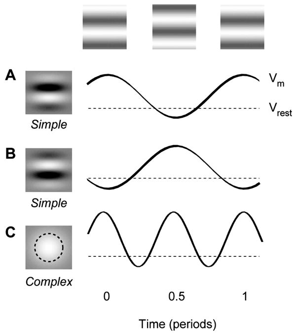
Responses of idealized simple and complex cells to a stimulus (a standing grating) whose contrast modulates sinusoidally in time. We illustrate the responses of three cells, whose receptive fields are shown in the left column. The dashed lines indicate the resting potential. (A) The membrane potential of a simple cell oscillates at the frequency of contrast reversal. (B) The oscillation will have the opposite sign in a second simple cell with a receptive field of opposite polarity. (C) The membrane potential of a complex cell oscillates at twice the frequency of the stimulus.
This reasoning is confirmed by observing the VSD responses to stimuli that periodically reverse in contrast (Figure 2). Gratings that contrast-reverse sinusoidally elicit responses that oscillate at twice the sinusoid’s frequency (Figure 2B,D). These 2nd harmonic responses can be accompanied by a 4th harmonic component (e.g. response to 5 Hz stimulus in Figure 2D); indeed, the traces often resembled triangular waveforms more than sinusoids.
Figure 2.

VSD responses to contrast-reversing stimuli, and basic properties of the 2nd harmonic response. (A) VSD signals measured in response to a blank screen, averaged over 10.6 mm2 of cortex. (B) VSD signals measured over the same area in response to a standing grating reversing in contrast at 3, 4, 5, 7, and 9 Hz. For graphical purposes, traces in A and B were high-pass filtered above 4 Hz. (C,D) Amplitude spectra of the responses in A,B. Gray traces show standard deviation measured by bootstrap over stimulus presentations (50 repeats). Dotted curve indicates 1/fx fit to amplitude spectrum of the noise shown in A. Stimuli elicited strong responses at twice the frequency of contrast reversal (2nd harmonic, arrows). (E) Amplitude of the 2nd harmonic response as a function of stimulus frequency. The gray area indicates a measure of noise level, the average amplitude at the frequencies near (±2 Hz) the 2nd harmonic. (F) Signal/noise ratios measured as z-scores (amplitude of the 2nd harmonic divided by noise level). (G) Average across 5 experiments of the z-scores, as a function of stimulus frequency. (H) Phase of the 2nd harmonic response as a function of stimulus frequency. The slope of the linear fit gives the integration time, 82 ms. Experiment 50-2-6.
Similar oscillations could be observed in the field potential throughout the depth of cortex (Supplementary Figure 1). Just as in VSD signals, in field potentials the 1st harmonic responses are negligible, and the 2nd harmonic responses are strong (Schroeder et al., 1991).
Frequency-dependence of VSD noise
Seeking to elicit strong VSD signals that stand out from the noise, we turned our attention to the properties of the noise. We measured the VSD responses to a uniform gray screen (“noise”), and studied how their amplitude depends on frequency (Figure 2C). Noise in VSD measurements is largest at low temporal frequencies (Arieli et al., 1995; Prechtl et al., 1997). We found that its amplitude decreases with the inverse of frequency: it was well fitted by the expression 1/fx, where f is frequency and the fitted exponent was x = 1.04 ± 0.06 (s.e., n = 6).
This dependence of noise on frequency agrees with the notion that most physiological sources of variability contribute power to low frequencies. Spontaneous vasomotor activity oscillates below 0.1 Hz (Kalatsky and Stryker, 2003) and respiration oscillates at 0.3–0.6 Hz. In the higher range of frequencies lies the large artifact caused by heart beats (Shoham et al., 1999), which oscillates at 2.5–4.2 Hz. These oscillations do not appear in the traces averaged across acquisition epochs (Figure 2C) because our data are acquired randomly in relation to heart beats and the contribution from different epochs cancel each other out. The remaining amplitude spectrum is likely to reflect mostly the ongoing cortical activity, i.e. all neural signals that are not synchronous with the stimulus (Arieli et al., 1996).
Amplitude spectra of the 1/f kind are commonly observed in human EEG (Pritchard, 1992). Indeed we observed them also in field potentials (Supplementary Figure 1). In response to a gray screen, the field potential shows large fluctuations, whose amplitude decreases with frequency. We fitted this amplitude with the same exponential expression as our VSD data, and found exponents of x = 1.00 ± 0.29 (s.e., n = 16).
Basic properties of 2nd harmonic responses
We then returned to the 2nd harmonic responses and asked at which stimulus frequencies they are most distinct from noise. The relationship between 2nd harmonic signal and noise depends on stimulus frequency (Figure 2E). Stimuli above 8–10 Hz typically elicited small responses, consistent with the preference of cat V1 neurons for frequencies <10 Hz (DeAngelis et al., 1993; Movshon et al., 1978b; Saul and Humphrey, 1992). Responses elicited by stimuli below ~3 Hz, conversely, overlapped with large noise components and were thus not easily measured. Between these extremes lie the stimuli reversing at 4–8 Hz, which elicit 2nd harmonic responses that are strong and have frequencies (8–16 Hz) high enough to clear the noise. On average, the optimal signal/noise was obtained at 5.2 ± 1.4 Hz (s.d. n = 5, Figure 2F,G). For subsequent experiments, therefore, we generally chose to stimulate at 5 Hz and to measure responses at 10 Hz.
The 2nd harmonic responses yield not only a measure of response magnitude, but also a measure of latency (Figure 2H). In sinusoidal responses, this latency can readily be measured from the sinusoid’s phase. For a pure delay, phase decreases linearly with frequency. Latencies are therefore estimated by fitting a line to graphs relating response phase to stimulus frequency. The slope of this line is known as integration time (Reid et al., 1992) and indicates the latency between the stimulus onset and the bulk of the resulting response. We found it to be rather uniform across experiments, 82 ms for the example experiment (Figure 2H) and 82 ± 5 ms on average (s.e., n = 4). Response latency in V1, however, is far from fixed and depends on factors such as contrast (Dean and Tolhurst, 1986), temporal content (Reid et al., 1992), and spatial content (Bredfeldt and Ringach, 2002; Frazor et al., 2004). Indeed, in a control experiment (not shown) we found the integration time to be ~60 ms longer at 10% contrast than at 100% contrast.
Maps of orientation selectivity from 2nd harmonic responses
The 2nd harmonic responses yielded high-quality maps of orientation preference (Figure 3). Stimuli of different orientation elicited the profiles of activity typical of cat V1 (Hübener and Bonhoeffer, 2002), with orthogonal orientations yielding complementary maps (Figure 3A–D). These profiles of activity could be combined to produce the characteristic map of orientation preference (Figure 3E).
Figure 3.

Maps of orientation preference obtained from 2nd harmonic responses. (AD) Amplitude of the 2nd harmonic responses to standing gratings with different orientations, whose contrast reversed at 5 Hz. For graphical purposes, these maps were corrected by subtracting the average response to 8 orientations (“cocktail correction”), and ignoring negative responses. (E) Map of orientation selectivity obtained from these responses (plus other 4 that are not shown). Color indicates preferred orientation, and saturation indicates tuning amplitude (see pinwheel inset). (F) Reference image of the cortex illuminated with green light. (G–J) The population responses in A–D expressed as a function of pixel preferred orientation (obtained from the map in E). The open symbols indicate responses to a gray screen. (K) The population response expressed as a function of angle between preferred orientation and stimulus orientation, obtained by averaging the responses in G–J and those to 4 additional orientations. Error bars are s.d. computed over 8 stimulus orientations. A Gaussian fit is superimposed (curve). (L) Same, for the amplitude of the 1st harmonic. (M) Same, for the mean of the responses (the 0th harmonic). Experiment 50-2-3.
The quality of these maps can be assessed from the population responses expressed as a function of preferred orientation (Figure 3G–J). Having labeled each pixel with an orientation preference (Figure 3E), we expressed the responses to individual stimulus orientations (Figure 3A–D) as a function of preferred orientation (Figure 3G–J). As expected, the responses are strongest in the pixels selective for the stimulus orientation and weakest in the pixels selective for the orthogonal orientation.
These results can be summarized by a single population response profile, where orientation preference is expressed relative to stimulus orientation (Figure 3K). To quantify this profile we fitted it with a circular Gaussian (Figure 3K, curve), and estimated the half width at half-height. The average value was 30 ± 5 deg (s.d., n = 14), comparable to the value (38 ± 15 deg) observed in the membrane potential of individual V1 neurons (Carandini and Ferster, 2000). An additional effect of the stimulus is an elevation of responses that is independent of orientation (Sharon and Grinvald, 2002): the trough in the profile of activation (Figure 3K) is substantially higher than the responses to a blank screen (Figure 3G–J, open symbols). A similar effect is seen in the membrane potential of complex cells, which show some depolarization in response to all orientations, including those orthogonal to the preferred (Carandini and Ferster, 2000).
The 2nd harmonic responses (Figure 3K) are much stronger and better tuned than the 1st harmonic responses (Figure 3L). This observation confirms an assumption that we had made in our argument for the cancellation of simple cell responses (Figure 1): that simple cells whose receptive fields have different polarity are not segregated over the scale resolved by VSD imaging (~100 μm). This assumption is reasonable because nearby simple cells can be selective for widely different spatial phases of a grating stimulus (DeAngelis et al., 1999; Pollen and Ronner, 1981).
The signals provided by the 2nd harmonic responses (Figure 3K) are also superior to those observed at the 0th harmonic, the mean of the responses over time (Figure 3M). One might expect a strong signal at this harmonic because simple and complex cells respond to sinusoidal stimuli not only with a modulated response, but also with an elevation in mean potential (Carandini and Ferster, 2000; Jagadeesh et al., 1993). Indeed, visual stimuli increase the VSD amplitude at the lower frequencies (Figure 2D). However, this increase does not seem to be appropriate for mapping purposes, as it is noisy and not discernibly tuned for orientation (Figure 3M). The noisiness and lack of selectivity of the 0th harmonic might result from this signal having to compete with the strong noise present at the low frequencies (Figure 2C).
Maps of retinotopy from 2nd harmonic responses
The 2nd harmonic responses could also be used to yield maps of retinotopy (Figure 4). We measured these maps by stimulating with contrast-reversing gratings framed by elongated rectangular windows presented at various positions (Figure 4A,B). Moving the stimulus from left to right caused concomitant changes in the profile of the activity (Figure 4C). Moving the stimulus from high to low caused the activity to move from posterior to anterior (Figure 4D). By combining the responses to all these stimuli we computed a map of retinotopy, which relates the visual field (Figure 4E) to the surface of the cortex (Figure 4F).
Figure 4.
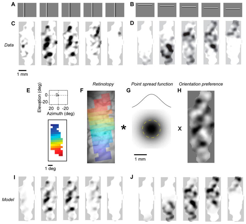
Maps of retinotopy obtained from 2nd harmonic responses and their relation to the orientation preference maps. (A–B) Stimuli were gratings windowed in narrow rectangles. (C–D) Amplitude of 2nd harmonic responses. The gray scale (white to black) spans the values between the 95th and 99th percentiles of the intensity distribution. (E–F) Map of retinotopy. The inset shows the region of visual field covered by the patch of cortex, in the same scale as the stimuli. (G) The point spread function estimated from data, which is modeled as a 2-D Gaussian. (H) Map of orientation preference (vertical minus horizontal). (I–J) Predictions of the model for the amplitude of 2nd harmonic responses. Gray scale as in C–D. Experiments 67-2-1 and 67-2-2.
The function underlying our maps of retinotopy is simple, but suffices for the job at hand (Figure 4E,F). This mapping function relates a point in visual space to a point in cortex. It is linear and is specified by only 4 parameters: the two Cartesian coordinates of the area centralis in cortex, the angle of rotation, and the magnification factor (see Methods). A first limitation of this mapping function is that it is one-to-one, which is appropriate for area 17 or 18 but not for the region that spans the two, where a point in retina corresponds to two points in cortex (Tusa et al., 1978; 1979). This concern is minor: our images mostly centered on one area, with at most a small region in the other area. A second limitation of our mapping function is that it is linear, which can only be appropriate in a local region of cortex; over the full extent of V1 the magnification factor shows great variation (Tusa et al., 1978; 1979). A more realistic logarithmic mapping function (Balasubramanian et al., 2002), however, costs additional parameters and did not noticeably improve the fits.
Relationship between retinotopy and orientation preference
The relationship between maps of orientation preference (Figure 3E) and of retinotopy (Figure 4F) has received substantial interest (Bosking et al., 2002). An essential factor in the combination of these maps is the point spread function, the extent of cortex that is activated by a pointwise visual stimulus. The point spread function has been calculated from measurements of receptive field size and magnification factor (Hubel and Wiesel, 1974); in cat its width averages 2.6 mm, regardless of eccentricity (Albus, 1975). The structure of orientation preference maps, however, is finer than this scale. Therefore, as has been illustrated recently (Bosking et al., 2002), a small oriented stimulus activates a region of cortex that is extended (because of the point spread function), but not uniform (because of the map of orientation preference). Indeed, our bar stimuli (Figure 4A,B), elicited responses that are broad and patchy (Figure 4C,D). The patchiness is due to the orientation map: when the combined responses to horizontal bars are subtracted from the combined responses to vertical bars, the result is a clear map of (horizontal vs. vertical) orientation preference (Figure 4H).
In summary, the pattern of activity elicited by an oriented stimulus must depend on the interplay of three factors, namely (1) the map of retinotopy; (2) the point spread function; and (3) the map of orientation preference. We asked what the exact rules of combination are for these three factors.
We tested a simple rule of combination. Our stimuli have uniform orientation and contrast inside a contour, and zero contrast outside the contour (Figure 4A,B). First, we predicted the representation of the contour in cortex based on the map of retinotopy (Figure 4E,F). The result is a tight region of activation with sharp borders. Second, we blurred this region of activation by convolving with the point spread function, which we modeled as a 2-dimensional Gaussian profile (Figure 4G). The result is a broad region of activation with blurred borders. Third, we multiplied point by point this region of activation with the map of preferred orientation, i.e. with the profile of activation expected for a large oriented stimulus (Figure 4H). The final result is a broad and patchy region of activation (Figure 4I,J).
This simple rule of combination provided good fits of the responses and allowed us to estimate the point spread function. The maps of activation predicted by the model (Figure 4I,J) closely resembled the actual responses (Figure 4C,D). The model explained 78 % of the variance for the data in our example experiment (Figure 4C,D), and 74 ± 8 % of the variance on average (s.d., n = 7). The estimated point spread function had a width (standard deviation) of 0.7 mm for the example experiment (Figure 4G), and 1.1 ± 0.4 mm across experiments (s.d., n = 7). The overall width of the estimated point spread function (~2.2 mm at two standard deviations) is consistent with the value of ~2.6 mm estimated with electrodes (Albus, 1975).
As a further validation of the model, we tested its performance on a new data set, one that was not used to obtain the model’s parameters (Supplementary Figure 2). We first obtained the model parameters from an experiment like the one described above (Figure 4). We then froze the parameters and asked whether the model could predict responses to a second stimulus set, which included not only horizontal and vertical gratings, but also diagonal ones. Reassuringly, the predictions of the model resembled the responses in all stimulus conditions (Supplementary Figure 2).
Traveling waves in the spatial domain
The activity that we elicit with contrast reversal of focal visual stimuli oscillates at twice the reversal frequency. Does this activity propagate away from the retinotopic representation of the stimulus? In other words, can the activity be described as a traveling wave?
To answer this question we examined an additional attribute of the 2nd harmonic responses: response phase (Figure 5). The 2nd harmonic responses are strong for the few stimuli placed near the optimal position, and decrease markedly as the stimulus is moved to more distal positions (Figure 5A,B). The phase of responses elicited distally differs from that of responses elicited proximally (Figure 5C): the color codes for phase are yellow and red when the stimulus excites the imaged region and progress towards purple, and cyan as the activated region becomes more distal and the associated response amplitudes become smaller. This progression is somewhat noisy due to small size of distal responses, but nonetheless suggests an increasing lag of the response as the distance between recorded regions and stimulated regions grows. This increasing lag is characteristic of a traveling wave.
Figure 5.
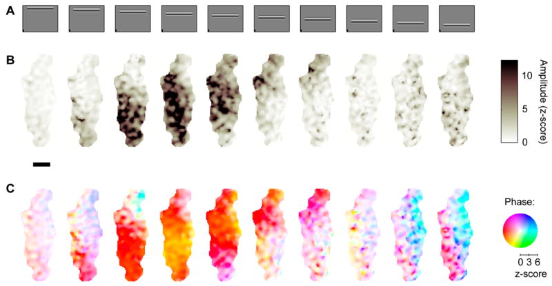
The oscillations in the 2nd harmonic responses have different phases depending on stimulus position. (A) Stimuli are the same as Figure 4. (B) Amplitude of 2nd harmonic responses (same data as in Figure 4D, only here it is shown in z-scores). (C) The phase of the 2nd harmonic responses depends on distance from the stimulated region of cortex. Phase is coded by color according to pinwheel shown in the right, with color saturation varying with response amplitude. As indicated by the scale below the pinwheel, the phases of responses with z-scores below about 2 are shown in white. Color-coded phase varies smoothly from yellow in regions that are retinotopically centered on the stimulus to red, purple, and then cyan in regions that are progressively more distant. Experiment 67-2-1.
To test the traveling wave hypothesis and characterize the speed of travel and other key properties, we summarized these data in a compact representation (Figure 6). This representation concentrates on a single dimension of space, and collapses all the stimulus conditions into one graph, thus simplifying the analysis and increasing the signal/noise ratio of our measurements. Having fitted the model of retinotopy (Figure 4E–F) we estimated the retinotopic location of the central axis of each stimulus, and expressed the amplitude of the 2nd harmonic responses (Figure 5B) as a function of distance from this location (Supplementary Figure 3). We could then create a composite of the responses to different stimuli (Figure 6A,B). As expected, activity is strongest in the retinotopic location of the stimulus, and decays gracefully as distance from this location increases (Figure 6A). Pooling across space and across stimuli allows us to estimate the phase of the responses with high accuracy even when the associated amplitudes are weak (Figure 6B). Crucially, the phase changes linearly with distance from the retinotopic location of the stimulus, consistent with travel at a constant speed of 0.30 m/s (Figure 6B).
Figure 6.
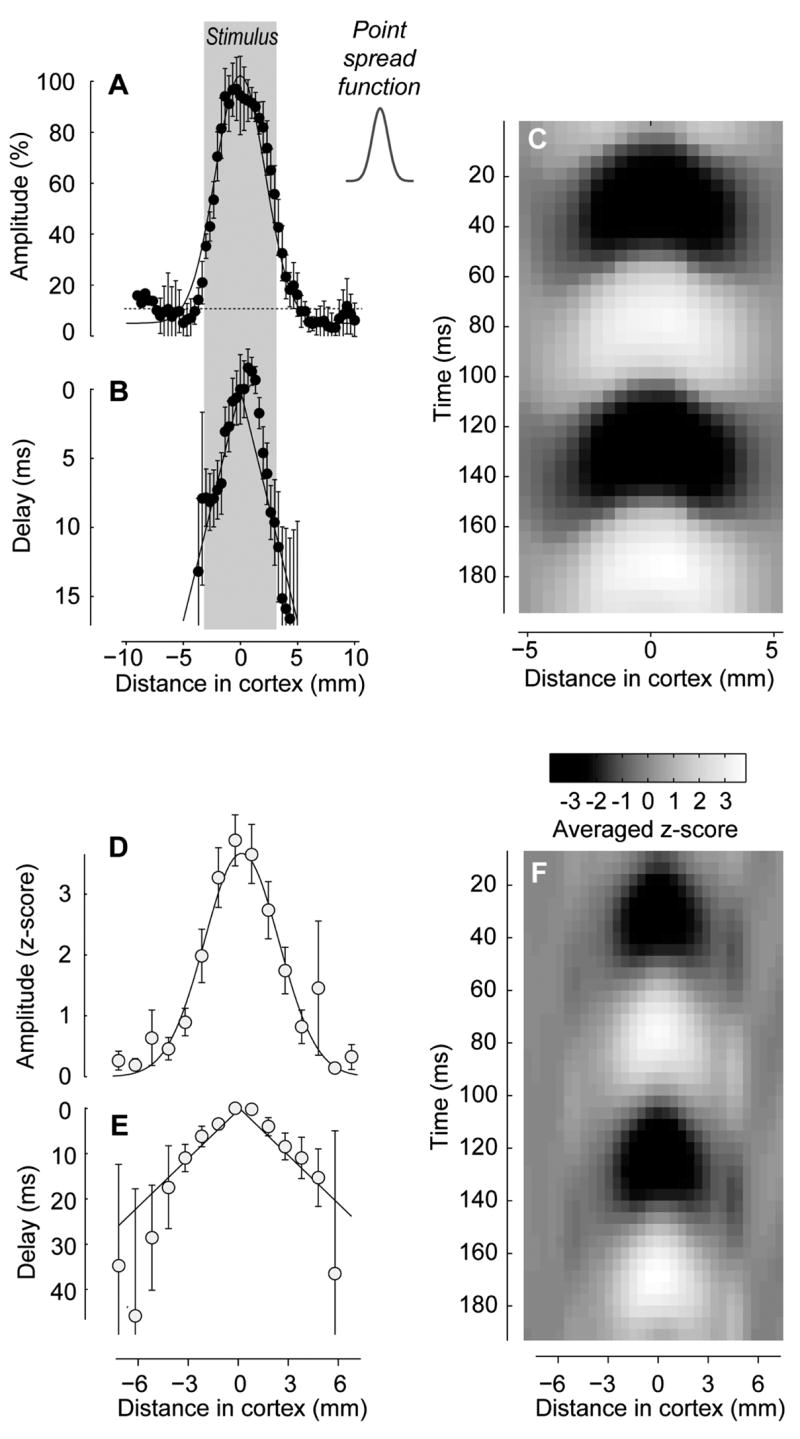
Traveling waves in the spatial domain. (A) Amplitude of the 2nd harmonic responses shown in Figure 5B, expressed as a function of distance from the retinotopic location of the stimulus. This representation collapses the two dimensions of cortex into one, and combines the contributions of all stimuli. The curve is a Gaussian fitted to the data (σ = 2.2 mm). The horizontal line indicates the average noise level. The gray region indicates the extent of the retinotopic representation of the stimulus in cortex. The inset shows the estimated points spread function for this experiment (σ = 0.7 mm) (B) The phase of these averaged 2nd harmonic responses, converted to delay in ms to facilitate the estimation of speed. The lines indicates the best linear fit (slope = 0.30 m/s). This fit was performed by imposing that the lines on each side of the origin have the same slope, and intercept at the origin at a value of zero. (C) The traveling wave in space-time. Activity is shown for one period of the stimulus (about 200 ms), averaged over periods and over repeats, and bandpass filtered at 7–13 Hz to emphasize the visually-driven responses. Gray levels go from −100% to 100%. (D–F) Same as A–C but averaged over 6 experiments. Gray levels indicate z-scores; they can be positive or negative, indicating standard deviations above or below the mean.
To further test the traveling wave hypothesis, we asked whether the phase lag seen with increased distance from the stimulated region is due to a delay in the whole time course of the oscillating responses. We averaged the responses over one cycle of the stimulus period (Figure 6C), and found the delay both in the onset and in the offset of the responses, as would be expected by a traveling wave.
The results were highly repeatable across 6 experiments (Figure 6D–F). The decay in wave amplitude with increasing distance extended over a couple of millimeters (Figure 6D). The corresponding increase in delay with increasing distance was well fitted by a line of constant speed (Figure 6E). The average speed was 0.28 m/s, with a 75% confidence interval of 0.19 to 0.55 m/s. The cycle averages of the responses pooled across experiments showed a progressive delay with distance from the origin (Figure 6F)
These results prompt a number of questions. Firstly, does the traveling wave have a trivial explanation? Perhaps there is a fixed relationship between response amplitude and phase, such that weak amplitudes are always associated with lagged phases. Secondly, is the traveling wave specific to cortical sites that are selective for different stimulus positions, or is it also seen across sites that differ in orientation preference?
Standing waves in the orientation domain
We address these questions by asking whether waves of activity travel also in the orientation domain (Figure 7). We consider the responses to contrast-reversing stimuli of different orientations, described earlier (Figure 3), and examine not only the amplitude of the 2nd harmonic (Figure 7A) but also its phase (Figure 7B). The analysis here is similar to the one performed in the spatial domain, except that we no longer consider the spatial dimension to be distance over the cortical surface but, rather, difference between preferred orientation and stimulus orientation.
Figure 7.
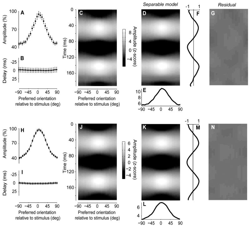
Standing waves in the orientation domain. (A) Amplitude of the 2nd harmonic responses as a function of angle between the preferred orientation and the stimulus orientation (as in Figure 3K). (B) Phase of these 2nd harmonic responses. (C) Space-time representation (as in Figure 6C, except that population responses are expressed as a function of preferred orientation rather than cortical distance). (D–F) The predictions of the best separable model, which is the product of a function of orientation in E and the time course in F. (G) The residual obtained by subtracting the model predictions in D from the responses in C. Experiment 50-2-3. (H–N) The same analysis, performed on the average of the responses in 23 experiments. Curve in H is a Gaussian fit.
The results of this analysis indicate that in the orientation domain the oscillatory activity is a standing wave (Figure 7B–G). The phase of the 2nd harmonic responses is independent of orientation, indicating that there are no delays in the responses of subpopulations tuned to different orientations (Figure 7B). Indeed, the profile of activation does not sharpen nor broaden through time, as can be observed by inspecting the responses in a space-time plot (Figure 7C). This plot is conceptually similar to the one obtained earlier in the spatial domain (Figure 6C), but its appearance is markedly different, as it lacks any hint of propagation. We confirmed these observations by fitting to the data the model of a standing wave. A standing wave is a separable function of orientation and space (Figure 7D), i.e. the product of a function of preferred orientation (Figure 7E) and a function of time (Figure 7F). This model fits the data well, as it leaves only a small residual (Figure 7G) and accounts for 98 % of the variance in the data in this example.
These results were highly repeatable across our 23 experiments (Figure 7H–N). The phase of the pooled 2nd harmonic responses was not affected by orientation (Figure 7H,I), and the pooled activity resembled a standing wave (Figure 7J), with the separable model accounting for 99.7% of the variance (Figure 7K–N). In individual data sets, the model explained over 90% of the variance in the 20/23 data sets obtained at high signal/noise (average z score of 6.7 ± 3.1) and accounted for less variance only in the 3/23 experiments with poor signal/noise ratios (average z score of 1.9 ± 1.7). This effect suggests that the modest missing variance is predominantly due to noise rather than to deviations from separability.
The standing wave observed in the orientation domain is not simply explained by the short distances between sites of differing orientation preference (Figure 8). Imagine that there were a traveling wave not only in the spatial domain but also in the orientation domain. This traveling wave might erroneously appear to us as a standing wave because the speeds are high and the cortical distances involved are short. To investigate this possibility we measured the average distance between sites in cortex as a function of difference in their preferred orientation. The average distance between a pixel and the closest pixel tuned to the orthogonal orientation is ~0.3 mm (Figure 8A–F). If activity in the orientation domain were a traveling wave propagating at 0.3 m/s (the speed seen in the spatial domain), the delay in activity between sites selective for orthogonal orientations would be ~1 ms. Could we detect such a small delay from our data? We simulated a wave that travels at 0.3 m/s across sites with different orientation preference, and compared these simulations to the data (Figure 8G). The two differ significantly: the measured delays lie on a flat line (consistent with a standing wave), and are all > 1 s.d. away from the predictions of the putative traveling wave. We can therefore reject the hypothesis of a wave that travels across the orientation domain.
Figure 8.

The standing wave observed in the orientation domain is not simply explained by the short distances between sites of differing orientation preference. (A) Map of orientation selectivity for an example hemisphere (experiment 50.2.3). (B) A 60 deg stimulus would excite preferentially these pixels, which are selective for 60±10 deg. (C) Map expressing for each pixel the distance to the closest pixel selective for 60±10 deg. (D) Average distance in this map, as a function of preferred orientation. (E) Average distance between a pixel and the nearest pixel with a given orientation preference, as a function of difference in preferred orientation between the two pixels. (F) Average of the results for 23 hemispheres (the gray area indicates 75% confidence intervals). (G) Comparison between the delay of the responses predicted by a putative traveling wave, and the delay measured in 23 hemispheres (phase of the responses expressed in ms). Based on the distribution in F, if activity traveled at a speed of 0.3 m/s (the value measured in the spatial domain), we should observe the distribution of response timings shown by the curve. The measured delays (data points), instead, lie more than 1 standard deviation away from the predictions of the putative traveling wave.
The marked difference between the waves in the spatial domain (Figure 6F) and in the orientation domain (Figure 7J) has a number of consequences. First, the traveling wave seen in the spatial domain is not simply due to a putative delay that might accompany weaker responses; it is truly a function of distance in cortex. Second, the circuits that underlie spatial selectivity and orientation selectivity are fundamentally different. The former distributes neural activity to a progressively larger group of neurons. The latter, instead, is balanced, so that the profile of activity neither sharpens nor broadens through time.
Discussion
Voltage-sensitive dye imaging in primary visual cortex is a powerful method to record the responses of neuronal populations. This method targets the superficial layers (Petersen et al., 2003a), which provide the main output to the rest of the cortex (Gilbert and Kelly, 1975). Moreover, our results indicate that this method reveals specifically the responses of complex cells.
VSD imaging of complex cells
The absence of simple cell responses from VSD signals can be explained by cancellation: the optical signal reflects primarily the membrane potential responses (rather than the spiking responses), and averages the responses of multiple simple cells, which cancel one another (Figure 1).
Indeed, there is ample reason to expect a substantial presence of simple-cell membrane in layers 2–3. Though it has been argued that simple cells occupy only layers 4 and 6 (Gilbert, 1977; Martinez et al., 2005), others found them widely present in layers 2/3 (Martin and Whitteridge, 1984), where they constitute 55% of neurons (Jacob et al., 2003). Moreover, layers 2/3 contain the apical dendrites of layer 5 pyramidal neurons, and even if these neurons were all complex, their dendrites might act as a simple cell (Mel et al., 1998).
The distinction we have made between simple and complex cells is based on their linearity of summation (Movshon et al., 1978a, c). This distinction is marked in the firing responses, but is blurred in the subthreshold responses: many cells are classified as simple in terms of firing responses, but give sizeable nonlinear responses in their membrane potential (Carandini and Ferster, 2000; Mechler and Ringach, 2002; Priebe et al., 2004). If the membrane potential of these cells responds with a noticeable 2nd harmonic to contrast-reversal, these cells might contribute to our VSD signals.
In fact, one of the reasons for the disagreement as to the layer specificity of simple and complex cells lies in the use of different definitions. For instance, a cell whose receptive field has a single subfield and whose operation is entirely linear would be called complex by some studies (Gilbert, 1977; Hubel and Wiesel, 1962; Martinez et al., 2005) and simple by others (Carandini and Ferster, 2000; Jacob et al., 2003; Mechler and Ringach, 2002; Priebe et al., 2004; Skottun et al., 1991).
Imaging forced oscillations
Having indicated complex cells as the main sources of VSD signals, we exploited this finding to elicit oscillations in cortex. These oscillations stood well clear of the noise, were easily imaged, and yielded high-resolution maps of functional architecture.
The key advantage of imaging periodic responses is the knowledge of the shape of the signal to be measured: a sinusoid of known frequency. One uses the whole time course of the response to estimate only two numbers, the amplitude and the phase of the sinusoid. With sufficient signal/noise, the latter can be measured with a precision that greatly surpasses the temporal resolution of the image acquisition. For example, most of our images were acquired at intervals of 9 ms and yet we were able to measure much subtler differences in delay across cortical positions (Figure 6).
These advantages of harmonic methods have long been exploited in the analysis of neural signals. Mapping with harmonic stimuli is the norm in measurements of visually-evoked EEG potentials (Regan and Regan, 1988; Zemon and Ratliff, 1982). Harmonic stimuli are also commonly used to establish retinotopy in fMRI measurements (Engel et al., 1997), and more recently in optical imaging of intrinsic signals (Kalatsky and Stryker, 2003).
Our approach may offer advantages over existing methods of VSD imaging. These methods prescribe procedures to reduce the impact of artifacts (Grinvald and Hildesheim, 2004; Sharon and Grinvald, 2002; Shoham et al., 1999). Repeatable artifacts are minimized by synchronizing stimuli and respirator with heart beat and by removing from the responses the control measurements made with a blank screen. Non-repeatable artifacts are tackled by subtracting from the responses a baseline obtained before the onset of each stimulus. This method rests on the assumption that noise varies slowly, so that artifacts are approximately constant during each stimulus presentation. It requires that stimuli be short (e.g. 300–500 ms), otherwise the baseline will not be a good estimate of the noise. Our methods allow us to use longer stimuli, without having to synchronize activity with the heart beat and without any concern for changes in heart rate over the course of the experiment.
Relationship between orientation preference and retinotopy
Having obtained high-resolution maps, we used these maps to investigate the interaction between orientation preference and retinotopy. It has long been clear that the profile of activation elicited in V1 by a stimulus that is localized and oriented depends on the map of retinotopy, on the point spread function, and on the map of orientation preference (Albus, 1975; Bosking et al., 2002; Hubel and Wiesel, 1974; Hübener and Bonhoeffer, 2002). It was not known, however, how these factors interact to yield the response to a given visual stimulus.
We described a simple rule of interaction that we found to be highly effective (Figure 4). This rule involves three steps, each of which can be interpreted in terms of anatomical connections and physiological mechanisms. We can think of the map of retinotopy as a map of projections from the visual field (through the lateral geniculate nucleus) to the cortex. The projection, however, is not from one point to another point, but rather from one point to a whole cloud of points: the center of the cloud is specified by the mapping function (step 1, Figure 4F), and the width of the cloud is specified by the point spread function (step 2, Figure 4G). A stimulus of a given orientation, in turn, will not excite all points in cortex, but only those whose preferred orientation matches the stimulus (step 3, Figure 4H). This could be because the cloud of connections is patchy (Mooser et al., 2004), or because V1 neurons do not integrate inputs from regions of the visual field that are inconsistent with their orientation selectivity (Alonso et al., 2001).
The success of simple pointwise multiplication indicates that for each pixel the selectivity for stimulus position was independent of stimulus orientation and the selectivity for stimulus orientation was independent of stimulus position. This independence in the effects of two stimulus attributes may seem to contradict the conflation of maps that has been recently reported (Basole et al., 2003). The two results, however, are complementary, and both follow from a widely accepted view of V1 selectivity based on local spatiotemporal receptive fields. Basole et al. (2003) imaged the responses to an oriented stimulus that was also moving; they could not simply predict those responses by multiplying the relevant maps (the one of orientation preference and the one of direction selectivity). This is precisely the result that would be expected if the selectivity of V1 neurons were due to a local spatiotemporal receptive field, as in such a mechanism the effects of orientation and direction are not independent (Mante and Carandini, 2005). We, in turn, imaged responses to an oriented stimulus that was also localized in space; we could indeed predict those responses by multiplying the relevant maps (the one of orientation preference and the one of retinotopy). Again, this is the result that could be expected if selectivity of V1 neurons were due to a local spatiotemporal receptive field: changing stimulus position would scale the responses of the receptive field with little effect on its selectivity for orientation.
A remaining open question concerns the degree to which the maps of orientation preference and retinotopy might influence or distort one another, perhaps in the interest of coverage (Blasdel and Campbell, 2001; Hubel and Wiesel, 1974; Swindale et al., 2000). An early study reported a strong dependence between the two maps (Das and Gilbert, 1997), but later studies argued otherwise (Bosking et al., 2002; Buzas et al., 2003), and recent anatomical results suggest that the map of retinotopy is in fact remarkably free from local distortions (Adams and Horton, 2003a; 2003b). Our methods lack the spatial resolution to address this question.
Standing waves in the orientation domain
Exploiting the high temporal resolution of our maps, we investigated the propagation of cortical activity in space and time. Our results indicate that within the retinotopic region of activation, cells of all orientation preferences are activated at the same time, rising to a peak response together (with the strength of the response varying with the preferred orientation) and decaying back down together. In other words, when measured in terms of orientation preference, the population responses neither sharpen nor broaden during the course of a response. Indeed, the population activity could be very well described by a separable model, the product of a function indicating the time course of the responses, and a function specifying their orientation selectivity. This separability is the definition of a standing wave.
These observations are fully consistent with earlier results obtained with VSD imaging (Sharon and Grinvald, 2002) and by recording from single neurons (Gillespie et al., 2001; Mazer et al., 2002). We did not find evidence for any sharpening of orientation selectivity over time, which had been reported by earlier studies (Ringach et al., 1997; Shevelev et al., 1993; Volgushev et al., 1995). These early measurements might be explained by a unified account: a relative decrease in a component of the response that is not tuned for orientation (Shapley et al., 2003).
In terms of circuitry, the standing wave might be explained by a balanced connectivity model, in which lateral excitation and inhibition have similar tuning, and therefore do not cause any sharpening or broadening of orientation selectivity (Anderson et al., 2000). It could also be explained by a completely feedforward model of orientations selectivity, one that dispenses with lateral connections between neurons selective for different orientations (Ferster and Miller, 2000).
Traveling waves in the spatial domain
When we measured activation by a focal visual stimulus at different retinotopic locations, we found that these locations show a sequence of activation and inactivation at different times. The results were well described by a dampened traveling wave propagating at constant speed of about 0.3 m/s.
These findings confirm earlier reports that activity in visual cortex spreads progressively over time. VSD measurements reveal that localized visual stimuli evoke activity over many millimeters of visual cortex, and this activity expands over time, with estimated speeds of 0.09–0.25 m/s in primate V1 (Grinvald et al., 1994) and 0.1 m/s in cat V1 (Arieli et al., 1995; Jancke et al., 2004). Such expanding cortical activity has been seen also with VSD imaging in vitro (Contreras and Llinas, 2001; Tanifuji et al., 1994; Tucker and Katz, 2003; Wu et al., 2001; Yuste et al., 1997) and in non-mammalian preparations (Prechtl et al., 1997; Senseman, 1999).
Our results extend the earlier reports by demonstrating that the spreading activity is indeed traveling, not just increasing in amplitude. The earlier studies concentrated on the effects of stimulus onset. The spread in activity that they discovered could have been the result of a standing wave: responses need to be larger than the noise to be measurable, and this criterion might be passed by a progressively larger region in the course of the response. By eliciting and measuring oscillating responses, we recorded responses to both stimulus onset and offset, and found that the offset is also delayed with distance from the stimulated region. This delay cannot be explained by a standing wave, and is characteristic of a traveling wave: the travel involves both the increase in activity that follows stimulus onset and the decrease in activity that follows stimulus offset.
This travel in activity is consistent with earlier electrophysiological measurements in cat V1. Local field potential measurements (Kitano et al., 1995) provided intriguing evidence for traveling activity over retinotopic location. Intracellular recordings provided further evidence, indicating that inputs from the periphery of the receptive field appear to reach a neuron after a delay (Bringuier et al., 1999). Interestingly, in these measurements the delay seems to depend on distance in the visual field and not on distance in cortex.
What is the biophysical substrate for the traveling wave? Ermentrout and Kleinfeld (2001) proposed three explanations for traveling waves in neural tissue. The first explanation invokes delayed excitation from a single oscillator: a region of cortex oscillates, it sends connections to other regions and these connections involve a delay that grows with distance. The second explanation invokes an excitable network that was initially quiescent: a region of cortex oscillates; it drives the activity of a nearby region, which starts oscillating and excites another nearby region, and so on. The third explanation invokes weakly coupled oscillators: all regions of cortex oscillate; the stimulated ones entrain the others to oscillate at a similar frequency, with a progressively delayed phase.
The simplest of these explanations is arguably the first one, especially because it finds a ready substrate in horizontal connections that abound in visual cortex. The speed of 0.2–0.5 m/s that we have estimated is highly consistent with the speed of action potential propagation along horizontal connections in cat V1 in vitro, which is 0.2–0.4 m/s (Hirsch and Gilbert, 1991). Similar speeds of horizontal connections have been seen in other preparations (Murakoshi et al., 1993; Nelson and Katz, 1995; Telfeian and Connors, 2003). Moreover, horizontal connections tend to favor sites with similar orientation preference (Bosking et al., 1997; Gilbert and Wiesel, 1989), possibly providing a support for the difference in dynamics that is seen across space and across orientation.
The second and third explanations would rely on less widely accepted biophysical substrates. Specifically, the third explanation has been invoked in other studies of wave propagation and oscillations in visual cortex (Ermentrout and Kleinfeld, 2001). However, in our study the oscillations were forced: we made the cortex oscillate in a certain region and we studied how this oscillation propagates. Under this condition, there is little reason to assume that the various regions of cortex oscillate on their own. If they do oscillate, however, then our results cannot be interpreted directly in terms of synaptic couplings. The interaction between oscillators, as measured from phase shifts, depends not only on synaptic connections but also on the stimulus (Grannan et al., 1993).
In conclusion, we suggest that the selectivity for stimulus orientation and position in V1 is served by fundamentally different schemes of connectivity. The connectivity underlying orientation selectivity achieves a balance between competition and distribution, so that activity involves a fixed set of neurons, with neither sharpening nor broadening of the activation profile: a standing wave. The connectivity underlying spatial selectivity is organized in a more distributive fashion, so that activity in response to a focal stimulus broadens to involve a progressively wider group of neurons with more disparate selectivity for spatial position: a traveling wave.
Experimental Procedures
Physiology
Young adult cats (2–4 Kg) were anesthetized first with Ketamine (22 mg/kg i/m) and Xylazine (1.1 mg/kg i/m) and then with Sodium Penthotal (0.5–2 mg/kg/hr i/v) and Fentanyl (typically 10 μg/kg/hr i/v), supplemented with inhalation of N2O (typically 70:30 with O2). A 1 cm craniotomy was performed over area V1 (usually area 18, occasionally area 17), centered on the midline. The eyes were treated with topical atropine and phenylephrine, and protected with contact lenses. A neuromuscular blocker was given to prevent eye movements (pancuronium bromide, 0.15 mg/kg/hr, i.v.). The animal was artificially respirated, and received periodic doses of an antibiotic (Cephazolin, 20 mg/kg IM, twice daily), of an anti-edematic steroid (Dexamethasone, 0.4 mg/kg daily), and of an anticholinergic agent (atropine sulfate, 0.05 mg/kg, i/m, daily). Fluid balance was maintained by intravenous infusion. The level of anesthesia was monitored through the EEG. Additional physiological parameters that were monitored include temperature, heart rate, end-tidal CO2, and lung pressure. Experiments typically lasted 48–72 hours. Procedures were approved by the Institutional Animal Care and Use Committee.
Stimuli
Stimuli were square gratings, presented monocularly on a CRT monitor (Sony Trinitron 500PS, refresh rate 125 Hz, mean luminance 32 cd/m2), modulating sinusoidally in contrast. The dominant spatial frequency was 0.2–0.4 cycles/deg, depending on the area imaged, and contrast was 50%. The windows were square (40×40 deg) for orientation experiments, and rectangular (typically 6×40 deg) for retinotopy experiments. Stimuli were preceded by ~2 s of uniform gray, typically lasted 1–2 s, and were presented in random order in blocks that were typically presented 10–20 times.
Imaging
Methods for VSD imaging were described by Grinvald and collaborators (Grinvald and Hildesheim, 2004; Sharon and Grinvald, 2002; Shoham et al., 1999). We stained the cortex with the VSD RH-1692 and imaged its fluorescence in 15–30 mm2 of V1. The dye was circulated in a chamber over the cortex for 3 hours, and washed out with saline. We acquired images with a CMOS digital camera (1M60 Dalsa, Waterloo, Ontario), as part of the Imager 3001 setup (Optical Imaging Inc, Rehovot, Israel). Images were acquired at a frame rate of 110 Hz, with spatial resolution of 28 μm per pixel. Additional spatial filtering was performed offline (bandpass, 0.2–2.2 cycles/mm). Frame acquisition was synchronized with the respirator. Illumination from a 100 W halogen light was delivered through two optic fibers. The excitation filter was bandpass at 630 ± 10 nm, and the emission filter was highpass, with cutoff at 665 nm.
Fourier analysis
To compute the amplitude spectra (Figure 2C–D), we averaged responses in a region of interest (ROI) where the mean optical response exceeded a criterion (80th percentile), and computed the FFT of the traces, averaging across repeats. Variability in these spectra was assessed via bootstrap over the stimulus repeats.
To compute a single Fourier component (e.g. the 2nd harmonic) we usually multiplied the traces by the appropriate complex exponential. The noise level was estimated by repeating the same procedure at frequencies at ± 2 Hz from the frequency of interest (e.g. gray area in Figure 2E). Z-scores were obtained by dividing the absolute value of the harmonic of interest by the amplitude of the estimated noise (e.g. Figure 2F).
Maps of orientation preference
Responses to stimuli of 8 orientations were combined in an orientation map that represents preferred orientation as hue, and orientation selectivity as saturation (Figure 3E). Preferred orientation and selectivity of pixel j were defined as angle(kj) and abs(kj), where , and θ1,…, θ8 are the orientations of the eight stimuli in radians.
Population responses (Figure 3G–M) were computed by ranking the pixels based on their orientation preference, and assigning each to one of 24 bins. The population response of a bin was the average response of the pixels belonging to the bin.
Maps of retinotopy
The mapping function that we use to describe retinotopy is best explained in the complex domain. It maps a point w = u+iv in the visual field to a point z = x+iy in cortex, given by
The parameters of the model are the magnification factor ρ (in mm/deg), the rotation angle φ (in radians), and the cortical coordinates z0 = x0+iy0 of the area centralis (w = 0). These four parameters, and the one parameter of the point spread function (the standard deviation σ), were found by carrying out a forward prediction of the data and minimizing the deviation between prediction and measurement.
The predictive model of responses (Figure 4) was defined as follows. Let θ be the stimulus orientation, and let the position and shape of the stimulus be defined by the distribution of contrast C(w), which is 1 inside the rectangle and 0 outside. Step 1 is to compute the cortical representation of the stimulus locations: r1(z) = C(f−1(z)), where f is the retinotopy mapping. Step 2 is to blur by convolving with the point spread function, r2(z) = [r1*Gσ](z), with Gσ a Gaussian with standard deviation σ. Step 3 is to multiply pointwise the result by the map of orientation preference r3(z) = r2(z)rθ(z), where rθ(z) is the response of pixel z to a full-field stimulus with orientation θ.
Space-time profiles of activity
Profiles of activity in space-time were obtained by averaging together the responses to different stimuli after appropriate translation (for pooling over stimulus position, e.g. Figure 6C) or rotation (for pooling over stimulus orientation, e.g. Figure 7C). The responses were averaged over cycles of the stimulus, and band-pass filtered (frequency of the 2nd harmonic ± 5 Hz) to concentrate on stimulus-driven responses. Z-score maps were obtained by dividing the mean cycle average by the standard deviation over cycles and orientations. The separable model (Figure 7K) was computed through Singular Value Decomposition, by multiplying the first row eigenvector by the first column eigenvector.
Supplementary Material
Supplementary Figure 1. Field Potential (FP) responses to flickering gratings. (A) A 16-channel polytrode (NeuroNexus, Inc) was inserted vertically into the cortex in the same area that was previously imaged. On the right, a schematic picture of the polytrode. (B) Cycle-average of the FP in response to a 5 Hz contrast-reversing grating. The FP oscillates at 10 Hz, twice the frequency of the stimulus. (C) Amplitude spectrum of the FP during the presentation of a blank stimulus. Black trace is the average amplitude (over 14 independent repeats) for the contact with the highest response to a grating (the one located at 1.1 mm depth in this example). The gray band is a confidence interval determined by bootstrapping over the independent repeats. Dotted curve indicates 1/fx fit to the amplitude spectrum of the noise (D) Same analysis as in C, but during the presentation of an oriented grating (60 deg), flickering at 5 Hz.
Supplementary Figure 2. Application of the retinotopy model to a novel stimulus. (A) The region of visual field covered by the patch of cortex. The gray rectangle (left) depicts the CRT monitor. (B) A map of retinotopy obtained from the 2nd harmonic responses to flickering gratings windowed in horizontal or vertical rectangles (as in Figure 4). The model explained 75.8% of the variance in this data set. Experiment 70-3-2/3. (C) In a control experiment, we used a stimulus composed of grating patches varying randomly in orientation and position. Some of these stimuli were vertical and horizontal, similar to those used to estimate the model in B. (D) The responses to these stimuli depends strongly on grating position and orientation. (E) The predictions of the model resemble the actual data. (F–H) As in C–E for additional stimuli in the control experiment. These stimuli were oblique, and thus are novel for the model. Though no similar stimuli appeared in the experiment used to obtain the model parameter, the model predictions resemble the actual responses. The model explained 51.3% of the variance in this novel data set. Experiment 70-3-8.
Supplementary Figure 3. Amplitude and phase of 2nd harmonic responses to individual stimuli. (A) Amplitude of responses as a function of stimulus position, for 8 stimulus positions (rows). These data are the same as those illustrated in Figure 5B, projected on one dimension of visual space. For each response, the corresponding Gaussian curve is shown, centered at the retinotopic location of the stimuli, as predicted by the model of retinotopy (Figure 4E,F). (B) The corresponding phases. The dotted lines are the predictions based on a traveling wave propagating at constant speed. Phases are shown only for data points with amplitude >20% (smaller responses have noisy phases) All of these responses can be aligned on the retinotopic position, and the results of this alignment are shown in Figure 6A,B. Once the alignment is done, the phases become less noisy even for locations that are up to 10 mm away from the stimulated region, providing even clearer support for the traveling wave hypothesis.
Acknowledgments
We thank Amiram Grinvald and his collaborators Dahlia Sharon and Shmuel Na’aman for training us in the technique of VSD imaging. We also thank Michael Stryker, Laila Dadvand, Rina Hildesheim, and Eyal Seidemann for technical advice, Vincent Bonin for help with the experiments, and Anthony Norcia, Daniel Adams, and Lawrence Sincich for suggestions and comments on the manuscript. Supported by an NRSA postdoctoral award (to RAF), by NEI grants R21-EY016441 and R01-EY017396, and by a Scholar Award from the McKnight Endowment Fund for Neuroscience.
Footnotes
Publisher's Disclaimer: This is a PDF file of an unedited manuscript that has been accepted for publication. As a service to our customers we are providing this early version of the manuscript. The manuscript will undergo copyediting, typesetting, and review of the resulting proof before it is published in its final citable form. Please note that during the production process errors may be discovered which could affect the content, and all legal disclaimers that apply to the journal pertain.
References
- Adams DL, Horton JC. A precise retinotopic map of primate striate cortex generated from the representation of angioscotomas. J Neurosci. 2003a;23:3771–3789. doi: 10.1523/JNEUROSCI.23-09-03771.2003. [DOI] [PMC free article] [PubMed] [Google Scholar]
- Adams DL, Horton JC. The representation of retinal blood vessels in primate striate cortex. J Neurosci. 2003b;23:5984–5997. doi: 10.1523/JNEUROSCI.23-14-05984.2003. [DOI] [PMC free article] [PubMed] [Google Scholar]
- Albus K. A quantitative study of the projection area of the central and the paracentral visual field in area 17 of the cat. I. The precision of the topography. Exp Brain Res. 1975;24:159–179. doi: 10.1007/BF00234061. [DOI] [PubMed] [Google Scholar]
- Alonso JM, Usrey WM, Reid RC. Rules of connectivity between geniculate cells and simple cells in cat primary visual cortex. J Neurosci. 2001;21:4002–4015. doi: 10.1523/JNEUROSCI.21-11-04002.2001. [DOI] [PMC free article] [PubMed] [Google Scholar]
- Anderson J, Carandini M, Ferster D. Orientation tuning of input conductance, excitation and inhibition in cat primary visual cortex. J Neurophysiol. 2000;84:909–931. doi: 10.1152/jn.2000.84.2.909. [DOI] [PubMed] [Google Scholar]
- Arieli A, Shoham D, Hildesheim R, Grinvald A. Coherent spatiotemporal patterns of ongoing activity revealed by real-time imaging coupled with single-unit recording in the cat visual cortex. J Neurophysiol. 1995;73:2072–2093. doi: 10.1152/jn.1995.73.5.2072. [DOI] [PubMed] [Google Scholar]
- Arieli A, Sterkin A, Grinvald A, Aertsen A. Dynamics of ongoing activity: explanation of the large variability in evoked cortical responses. Science. 1996;273:1868–1871. doi: 10.1126/science.273.5283.1868. [DOI] [PubMed] [Google Scholar]
- Balasubramanian M, Polimeni J, Schwartz EL. The V1-V2-V3 complex: quasiconformal dipole maps in primate striate and extra-striate cortex. Neural Networks. 2002;15:1157–1163. doi: 10.1016/s0893-6080(02)00094-1. [DOI] [PubMed] [Google Scholar]
- Basole A, White LE, Fitzpatrick D. Mapping multiple features in the population response of visual cortex. Nature. 2003;423:986–990. doi: 10.1038/nature01721. [DOI] [PubMed] [Google Scholar]
- Blasdel G, Campbell D. Functional retinotopy of monkey visual cortex. J Neurosci. 2001;21:8286–8301. doi: 10.1523/JNEUROSCI.21-20-08286.2001. [DOI] [PMC free article] [PubMed] [Google Scholar]
- Bosking WH, Crowley JC, Fitzpatrick D. Spatial coding of position and orientation in primary visual cortex. Nat Neurosci. 2002;5:874–882. doi: 10.1038/nn908. [DOI] [PubMed] [Google Scholar]
- Bosking WH, Zhang Y, Schofield B, Fitzpatrick D. Orientation selectivity and the arrangement of horizontal connections in tree shrew striate cortex. J Neurosci. 1997;17:2112–2127. doi: 10.1523/JNEUROSCI.17-06-02112.1997. [DOI] [PMC free article] [PubMed] [Google Scholar]
- Bredfeldt CE, Ringach DL. Dynamics of spatial frequency tuning in macaque V1. J Neurosci. 2002;22:1976–1984. doi: 10.1523/JNEUROSCI.22-05-01976.2002. [DOI] [PMC free article] [PubMed] [Google Scholar]
- Bringuier V, Chavane F, Glaeser L, Fregnac Y. Horizontal propagation of visual activity in the synaptic integration field of area 17 neurons. Science. 1999;283:695–699. doi: 10.1126/science.283.5402.695. [DOI] [PubMed] [Google Scholar]
- Buzas P, Volgushev M, Eysel UT, Kisvarday ZF. Independence of visuotopic representation and orientation map in the visual cortex of the cat. Eur J Neurosci. 2003;18:957–968. doi: 10.1046/j.1460-9568.2003.02808.x. [DOI] [PubMed] [Google Scholar]
- Carandini M, Ferster D. Membrane potential and firing rate in cat primary visual cortex. J Neurosci. 2000;20:470–484. doi: 10.1523/JNEUROSCI.20-01-00470.2000. [DOI] [PMC free article] [PubMed] [Google Scholar]
- Contreras D, Llinas R. Voltage-sensitive dye imaging of neocortical spatiotemporal dynamics to afferent activation frequency. J Neurosci. 2001;21:9403–9413. doi: 10.1523/JNEUROSCI.21-23-09403.2001. [DOI] [PMC free article] [PubMed] [Google Scholar]
- Das A, Gilbert CD. Distortions of visuotopic map match orientation singularities in primary visual cortex. Nature. 1997;387:594–598. doi: 10.1038/42461. [DOI] [PubMed] [Google Scholar]
- Dean AF, Tolhurst DJ. Factors influencing the temporal phase of response to bar and grating stimuli for simple cells in the cat striate cortex. Exp Br Res. 1986;62:143–151. doi: 10.1007/BF00237410. [DOI] [PubMed] [Google Scholar]
- DeAngelis GC, Ghose GM, Ohzawa I, Freeman RD. Functional micro-organization of primary visual cortex: receptive field analysis of nearby neurons. J Neurosci. 1999;19:4046–4064. doi: 10.1523/JNEUROSCI.19-10-04046.1999. [DOI] [PMC free article] [PubMed] [Google Scholar]
- DeAngelis GC, Ohzawa I, Freeman RD. Spatiotemporal organization of simple-cell receptive fields in the cat’s striate cortex. I. General characteristics and postnatal development. J Neurophysiol. 1993;69:1091–1117. doi: 10.1152/jn.1993.69.4.1091. [DOI] [PubMed] [Google Scholar]
- Engel SA, Glover GH, Wandell BA. Retinotopic organization in human visual cortex and the spatial precision of functional MRI. Cereb Cortex. 1997;7:181–192. doi: 10.1093/cercor/7.2.181. [DOI] [PubMed] [Google Scholar]
- Ermentrout GB, Kleinfeld D. Traveling electrical waves in cortex: insights from phase dynamics and speculation on a computational role. Neuron. 2001;29:33–44. doi: 10.1016/s0896-6273(01)00178-7. [DOI] [PubMed] [Google Scholar]
- Ferster D, Miller KD. Neural mechanisms of orientation selectivity in the visual cortex. Annu Rev Neurosci. 2000;23:441–471. doi: 10.1146/annurev.neuro.23.1.441. [DOI] [PubMed] [Google Scholar]
- Frazor RA, Albrecht DG, Geisler WS, Crane AM. Visual cortex neurons of monkeys and cats: temporal dynamics of the spatial frequency response function. J Neurophysiol. 2004;91:2607–2627. doi: 10.1152/jn.00858.2003. [DOI] [PubMed] [Google Scholar]
- Gilbert CD. Laminar differences in receptive properties of cells in cat primary visual cortex. J Physiol (London) 1977;268:391–421. doi: 10.1113/jphysiol.1977.sp011863. [DOI] [PMC free article] [PubMed] [Google Scholar]
- Gilbert CD, Kelly JP. The projections of cells in different layers of the cat’s visual cortex. Journal of Comparative Neurology. 1975;163:81–106. doi: 10.1002/cne.901630106. [DOI] [PubMed] [Google Scholar]
- Gilbert CD, Wiesel TN. Columnar specificity of intrinsic horizontal and corticocortical connections in cat visual cortex. J Neurosci. 1989;9:2432–2442. doi: 10.1523/JNEUROSCI.09-07-02432.1989. [DOI] [PMC free article] [PubMed] [Google Scholar]
- Gillespie DC, Lampl I, Anderson JS, Ferster D. Dynamics of the orientation-tuned membrane potential response in cat primary visual cortex. Nat Neurosci. 2001;4:1014–1019. doi: 10.1038/nn731. [DOI] [PubMed] [Google Scholar]
- Grannan ER, Kleinfeld D, Sompolinsky H. Stimulus-Dependent Synchronization of Neuronal Assemblies. Neural Comput. 1993;5:550–569. [Google Scholar]
- Grinvald A, Hildesheim R. VSDI: a new era in functional imaging of cortical dynamics. Nat Rev Neurosci. 2004;5:874–885. doi: 10.1038/nrn1536. [DOI] [PubMed] [Google Scholar]
- Grinvald A, Lieke EE, Frostig RD, Hildesheim R. Cortical point-spread function and long-range lateral interactions revealed by real-time optical imaging of macaque monkey primary visual cortex. J Neurosci. 1994;14:2545–2568. doi: 10.1523/JNEUROSCI.14-05-02545.1994. [DOI] [PMC free article] [PubMed] [Google Scholar]
- Hirsch JA, Gilbert CD. Synaptic physiology of horizontal connections in the cat’s visual cortex. J Neurosci. 1991;11:1800–1809. doi: 10.1523/JNEUROSCI.11-06-01800.1991. [DOI] [PMC free article] [PubMed] [Google Scholar]
- Hubel DH, Wiesel TN. Receptive fields, binocular interaction and functional architecture in the cat’s visual cortex. Journal of Physiology (London) 1962;160:106–154. doi: 10.1113/jphysiol.1962.sp006837. [DOI] [PMC free article] [PubMed] [Google Scholar]
- Hubel DH, Wiesel TN. Uniformity of monkey striate cortex: a parallel relationship between field size, scatter, and magnification factor. J Comp Neurol. 1974;158:295–305. doi: 10.1002/cne.901580305. [DOI] [PubMed] [Google Scholar]
- Hübener M, Bonhoeffer T. Optical imaging of functional architecture in cat primary visual cortex. In: Payne BR, Peters A, editors. The cat primary visual cortex. New York: Academic Press; 2002. pp. 1–137. [Google Scholar]
- Jacob MS, Peterson MR, Wu A, Freeman RD. Laminar differences in response characteristics of cells in the primary visual cortex. Washington, DC: Society for Neuroscience; 2003. Program No. 910.13. In Online Abstract Viewer. [Google Scholar]
- Jagadeesh B, Wheat HS, Ferster D. Linearity of summation of synaptic potentials underlying direction selectivity in simple cells of the cat visual cortex. Science. 1993;262:1901–1904. doi: 10.1126/science.8266083. [DOI] [PubMed] [Google Scholar]
- Jancke D, Chavane F, Naaman S, Grinvald A. Imaging cortical correlates of illusion in early visual cortex. Nature. 2004;428:423–426. doi: 10.1038/nature02396. [DOI] [PubMed] [Google Scholar]
- Kalatsky VA, Stryker MP. New paradigm for optical imaging: temporally encoded maps of intrinsic signal. Neuron. 2003;38:529–545. doi: 10.1016/s0896-6273(03)00286-1. [DOI] [PubMed] [Google Scholar]
- Kitano M, Kasamatsu T, Norcia AM, Sutter EE. Spatially distributed responses induced by contrast reversal in cat visual cortex. Exp Brain Res. 1995;104:297–309. doi: 10.1007/BF00242015. [DOI] [PubMed] [Google Scholar]
- Mante V, Carandini M. Mapping of stimulus energy in primary visual cortex. J Neurophysiol. 2005;94:788–798. doi: 10.1152/jn.01094.2004. [DOI] [PubMed] [Google Scholar]
- Martin KA, Whitteridge D. Form, function, and intracortical projections of spiny neurons in the striate visual cortex of the cat. Journal of Physiology (London) 1984;353:463–504. doi: 10.1113/jphysiol.1984.sp015347. [DOI] [PMC free article] [PubMed] [Google Scholar]
- Martinez LM, Wang Q, Reid RC, Pillai C, Alonso JM, Sommer FT, Hirsch JA. Receptive field structure varies with layer in the primary visual cortex. Nat Neurosci. 2005;8:372–379. doi: 10.1038/nn1404. [DOI] [PMC free article] [PubMed] [Google Scholar]
- Mazer JA, Vinje WE, McDermott J, Schiller PH, Gallant JL. Spatial frequency and orientation tuning dynamics in area V1. Proc Natl Acad Sci USA. 2002;99:1645–1650. doi: 10.1073/pnas.022638499. [DOI] [PMC free article] [PubMed] [Google Scholar]
- Mechler F, Ringach DL. On the classification of simple and complex cells. Vision Res. 2002;42:1017–1033. doi: 10.1016/s0042-6989(02)00025-1. [DOI] [PubMed] [Google Scholar]
- Mel BW, Ruderman DL, Archie KA. Translation-invariant orientation tuning in visual “complex” cells could derive from intradendritic computations. J Neurosci. 1998;18:4325–4334. doi: 10.1523/JNEUROSCI.18-11-04325.1998. [DOI] [PMC free article] [PubMed] [Google Scholar]
- Mooser F, Bosking WH, Fitzpatrick D. A morphological basis for orientation tuning in primary visual cortex. Nat Neurosci. 2004;7:872–879. doi: 10.1038/nn1287. [DOI] [PubMed] [Google Scholar]
- Movshon JA, Thompson ID, Tolhurst DJ. Nonlinear spatial summation in the receptive fields of complex cells in the cat striate cortex. J Physiol (London) 1978a;283:78–100. doi: 10.1113/jphysiol.1978.sp012488. [DOI] [PMC free article] [PubMed] [Google Scholar]
- Movshon JA, Thompson ID, Tolhurst DJ. Spatial and temporal contrast sensitivity of neurones in areas 17 and 18 of the cat’s visual cortex. Journal of Physiology (London) 1978b;283:101–120. doi: 10.1113/jphysiol.1978.sp012490. [DOI] [PMC free article] [PubMed] [Google Scholar]
- Movshon JA, Thompson ID, Tolhurst DJ. Spatial summation in the receptive fields of simple cells in the cat’s striate cortex. Journal of Physiology (London) 1978c;283:53–77. doi: 10.1113/jphysiol.1978.sp012488. [DOI] [PMC free article] [PubMed] [Google Scholar]
- Murakoshi T, Guo JZ, Ichinose T. Electrophysiological identification of horizontal synaptic connections in rat visual cortex in vitro. Neurosci Lett. 1993;163:211–214. doi: 10.1016/0304-3940(93)90385-x. [DOI] [PubMed] [Google Scholar]
- Nelson DA, Katz LC. Emergence of functional circuits in ferret visual cortex visualized by optical imaging. Neuron. 1995;15:23–34. doi: 10.1016/0896-6273(95)90061-6. [DOI] [PubMed] [Google Scholar]
- Petersen CC, Grinvald A, Sakmann B. Spatiotemporal dynamics of sensory responses in layer 2/3 of rat barrel cortex measured in vivo by voltage-sensitive dye imaging combined with whole-cell voltage recordings and neuron reconstructions. J Neurosci. 2003a;23:1298–1309. doi: 10.1523/JNEUROSCI.23-04-01298.2003. [DOI] [PMC free article] [PubMed] [Google Scholar]
- Petersen CC, Hahn TT, Mehta M, Grinvald A, Sakmann B. Interaction of sensory responses with spontaneous depolarization in layer 2/3 barrel cortex. Proc Natl Acad Sci U S A. 2003b;100:13638–13643. doi: 10.1073/pnas.2235811100. [DOI] [PMC free article] [PubMed] [Google Scholar]
- Pollen DA, Ronner SF. Phase relationship between adjacent simple cells in the visual cortex. Science. 1981;212:1409–1411. doi: 10.1126/science.7233231. [DOI] [PubMed] [Google Scholar]
- Prechtl JC, Cohen LB, Pesaran B, Mitra PP, Kleinfeld D. Visual stimuli induce waves of electrical activity in turtle cortex. Proc Natl Acad Sci U S A. 1997;94:7621–7626. doi: 10.1073/pnas.94.14.7621. [DOI] [PMC free article] [PubMed] [Google Scholar]
- Priebe NJ, Mechler F, Carandini M, Ferster D. The contribution of spike threshold to the dichotomy of cortical simple and complex cells. Nat Neurosci. 2004;7:1113–1122. doi: 10.1038/nn1310. [DOI] [PMC free article] [PubMed] [Google Scholar]
- Pritchard WS. The brain in fractal time: 1/f-like power spectrum scaling of the human electroencephalogram. Int J Neurosci. 1992;66:119–129. doi: 10.3109/00207459208999796. [DOI] [PubMed] [Google Scholar]
- Regan D, Regan MP. Objective evidence for phase-independent spatial frequency analysis in the human visual pathway. Vision Res. 1988;28:187–191. [PubMed] [Google Scholar]
- Reid RC, Victor JD, Shapley RM. Broadband temporal stimuli decrease the integration time of neuron in cat striate cortex. Vis Neurosci. 1992;9:39–45. doi: 10.1017/s0952523800006350. [DOI] [PubMed] [Google Scholar]
- Ringach DL, Bredfeldt CE, Shapley RM, Hawken MJ. Suppression of neural responses to nonoptimal stimuli correlates with tuning selectivity in macaque V1. J Neurophysiol. 2002;87:1018–1027. doi: 10.1152/jn.00614.2001. [DOI] [PubMed] [Google Scholar]
- Ringach DL, Hawken MJ, Shapley R. Dynamics of orientation tuning in macaque primary visual cortex. Nature. 1997;387:281–284. doi: 10.1038/387281a0. [DOI] [PubMed] [Google Scholar]
- Saul AB, Humphrey AL. Temporal-frequency tuning of direction selectivity in cat visual cortex. Vis Neurosci. 1992;8:365–372. doi: 10.1017/s0952523800005101. [DOI] [PubMed] [Google Scholar]
- Schroeder CE, Tenke CE, Givre SJ, Arezzo JC, Vaughan HG., Jr Striate cortical contribution to the surface-recorded pattern-reversal VEP in the alert monkey. Vision Res. 1991;31:1143–1157. doi: 10.1016/0042-6989(91)90040-c. [DOI] [PubMed] [Google Scholar]
- Senseman DM. Spatiotemporal structure of depolarization spread in cortical pyramidal cell populations evoked by diffuse retinal light flashes. Vis Neurosci. 1999;16:65–79. doi: 10.1017/s0952523899161030. [DOI] [PubMed] [Google Scholar]
- Shapley R, Hawken M, Ringach DL. Dynamics of orientation selectivity in the primary visual cortex and the importance of cortical inhibition. Neuron. 2003;38:689–699. doi: 10.1016/s0896-6273(03)00332-5. [DOI] [PubMed] [Google Scholar]
- Sharon D, Grinvald A. Dynamics and constancy in cortical spatiotemporal patterns of orientation processing. Science. 2002;295:512–515. doi: 10.1126/science.1065916. [DOI] [PubMed] [Google Scholar]
- Sharon D, Jancke D, Chavane F, Na’aman S, Grinvald A. Cortical Response Field Dynamics in Cat Visual Cortex. Cereb Cortex. 2007 doi: 10.1093/cercor/bhm019. [DOI] [PubMed] [Google Scholar]
- Shevelev IA, Sharaev GA, Lazareva NA, Novikova RV, Tikhomirov AS. Dynamics of orientation tuning in the cat striate cortex neurons. Neuroscience. 1993;56:865–876. doi: 10.1016/0306-4522(93)90133-z. [DOI] [PubMed] [Google Scholar]
- Shoham D, Glaser DE, Arieli A, Kenet T, Wijnbergen C, Toledo Y, Hildesheim R, Grinvald A. Imaging cortical dynamics at high spatial and temporal resolution with novel blue voltage-sensitive dyes. Neuron. 1999;24:791–802. doi: 10.1016/s0896-6273(00)81027-2. [DOI] [PubMed] [Google Scholar]
- Skottun BC, De Valois RL, Grosof DH, Movshon JA, Albrecht DG, Bonds AB. Classifying simple and complex cells on the basis of response modulation. Vis Res. 1991;31:1079–1086. doi: 10.1016/0042-6989(91)90033-2. [DOI] [PubMed] [Google Scholar]
- Swindale NV, Shoham D, Grinvald A, Bonhoeffer T, Hubener M. Visual cortex maps are optimized for uniform coverage. Nat Neurosci. 2000;3:822–826. doi: 10.1038/77731. [DOI] [PubMed] [Google Scholar]
- Tanifuji M, Sugiyama T, Murase K. Horizontal propagation of excitation in rat visual cortical slices revealed by optical imaging. Science. 1994;266:1057–1059. doi: 10.1126/science.7973662. [DOI] [PubMed] [Google Scholar]
- Telfeian AE, Connors BW. Widely integrative properties of layer 5 pyramidal cells support a role for processing of extralaminar synaptic inputs in rat neocortex. Neurosci Lett. 2003;343:121–124. doi: 10.1016/s0304-3940(03)00379-3. [DOI] [PubMed] [Google Scholar]
- Tucker TR, Katz LC. Spatiotemporal patterns of excitation and inhibition evoked by the horizontal network in layer 2/3 of ferret visual cortex. J Neurophysiol. 2003;89:488–500. doi: 10.1152/jn.00869.2001. [DOI] [PubMed] [Google Scholar]
- Tusa RJ, Palmer LA, Rosenquist AC. The retinotopic organization of area 17 (striate cortex) in the cat. J Comp Neurol. 1978;177:213–236. doi: 10.1002/cne.901770204. [DOI] [PubMed] [Google Scholar]
- Tusa RJ, Rosenquist AC, Palmer LA. Retinotopic organization of areas 18 and 19 in the cat. J Comp Neurol. 1979;185:657–678. doi: 10.1002/cne.901850405. [DOI] [PubMed] [Google Scholar]
- Volgushev M, Vidyasagar TR, Pei X. Dynamics of the orientation tuning of postsynaptic potentials in the cat visual cortex. Vis Neurosci. 1995;12:621–628. doi: 10.1017/s0952523800008919. [DOI] [PubMed] [Google Scholar]
- Wu JY, Guan L, Bai L, Yang Q. Spatiotemporal properties of an evoked population activity in rat sensory cortical slices. J Neurophysiol. 2001;86:2461–2474. doi: 10.1152/jn.2001.86.5.2461. [DOI] [PubMed] [Google Scholar]
- Yuste R, Tank DW, Kleinfeld D. Functional study of the rat cortical microcircuitry with voltage- sensitive dye imaging of neocortical slices. Cereb Cortex. 1997;7:546–558. doi: 10.1093/cercor/7.6.546. [DOI] [PubMed] [Google Scholar]
- Zemon V, Ratliff F. Visual evoked potentials: evidence for lateral interactions. Proc Natl Acad Sci U S A. 1982;79:5723–5726. doi: 10.1073/pnas.79.18.5723. [DOI] [PMC free article] [PubMed] [Google Scholar]
Associated Data
This section collects any data citations, data availability statements, or supplementary materials included in this article.
Supplementary Materials
Supplementary Figure 1. Field Potential (FP) responses to flickering gratings. (A) A 16-channel polytrode (NeuroNexus, Inc) was inserted vertically into the cortex in the same area that was previously imaged. On the right, a schematic picture of the polytrode. (B) Cycle-average of the FP in response to a 5 Hz contrast-reversing grating. The FP oscillates at 10 Hz, twice the frequency of the stimulus. (C) Amplitude spectrum of the FP during the presentation of a blank stimulus. Black trace is the average amplitude (over 14 independent repeats) for the contact with the highest response to a grating (the one located at 1.1 mm depth in this example). The gray band is a confidence interval determined by bootstrapping over the independent repeats. Dotted curve indicates 1/fx fit to the amplitude spectrum of the noise (D) Same analysis as in C, but during the presentation of an oriented grating (60 deg), flickering at 5 Hz.
Supplementary Figure 2. Application of the retinotopy model to a novel stimulus. (A) The region of visual field covered by the patch of cortex. The gray rectangle (left) depicts the CRT monitor. (B) A map of retinotopy obtained from the 2nd harmonic responses to flickering gratings windowed in horizontal or vertical rectangles (as in Figure 4). The model explained 75.8% of the variance in this data set. Experiment 70-3-2/3. (C) In a control experiment, we used a stimulus composed of grating patches varying randomly in orientation and position. Some of these stimuli were vertical and horizontal, similar to those used to estimate the model in B. (D) The responses to these stimuli depends strongly on grating position and orientation. (E) The predictions of the model resemble the actual data. (F–H) As in C–E for additional stimuli in the control experiment. These stimuli were oblique, and thus are novel for the model. Though no similar stimuli appeared in the experiment used to obtain the model parameter, the model predictions resemble the actual responses. The model explained 51.3% of the variance in this novel data set. Experiment 70-3-8.
Supplementary Figure 3. Amplitude and phase of 2nd harmonic responses to individual stimuli. (A) Amplitude of responses as a function of stimulus position, for 8 stimulus positions (rows). These data are the same as those illustrated in Figure 5B, projected on one dimension of visual space. For each response, the corresponding Gaussian curve is shown, centered at the retinotopic location of the stimuli, as predicted by the model of retinotopy (Figure 4E,F). (B) The corresponding phases. The dotted lines are the predictions based on a traveling wave propagating at constant speed. Phases are shown only for data points with amplitude >20% (smaller responses have noisy phases) All of these responses can be aligned on the retinotopic position, and the results of this alignment are shown in Figure 6A,B. Once the alignment is done, the phases become less noisy even for locations that are up to 10 mm away from the stimulated region, providing even clearer support for the traveling wave hypothesis.