Maximizing power in seroepidemiological studies through the use of the proportional odds model

Abstract

Epidemiological studies of zoonotic influenza and other infectious diseases often rely upon analysis of levels of antibody titer. In most of these studies, the antibody titer data are dichotomized based on a chosen cut‐point and analyzed with a traditional binary logistic regression. However, cut‐points are often arbitrary, particularly those selected for rare diseases or for infections for which serologic assays are imperfect. Alternatively, the data can be left in the original form, as ordinal levels of antibody titer, and analyzed using the proportional odds model. We show why this approach yields superior power to detect risk factors. Additionally, we illustrate the advantages of using the proportional odds model with the analyses of zoonotic influenza antibody titer data.

Introduction

Antibody titer is often an important diagnostic tool in epidemiologically assessing infections, especially in retrospective and prospective studies where infection may be sub‐clinical. Such is the case for epidemiological studies of influenza infection where laboratory methods such as microneutralization and hemagglutination inhibition are used. ¹ Although the concentration of antibodies in sera is actually continuous, the use of some methods based on titers often produces data that are categorized into ordinal levels. For example, if the antibody concentration is so low that antibodies cannot be detected at a dilution of 1:10, then the concentration is recorded as ‘<1:10’. If the antibody is detected at a dilution of 1:10 but not at a dilution of 1:20, then the concentration is recorded as ‘1:10’. Thus, data are recorded in a sequence of titer categories (e.g. <1:10, 1:10, 1:20, 1:40, etc.), composing an ordinal response.

Often in examining titer data, a cut‐point is selected to dichotomize the response into a simple classification of disease vs. non‐disease. In outbreak situations, cut‐points are useful in estimating the number of cases or in searching for risk factors for infection. However, cut‐points are often arbitrary, particularly those selected for rare diseases or for infections for which serologic assays are imperfect. For example, considering serologic testing for a H1N1 avian influenza virus, antibody detection may be influenced by a subtle mismatch in wild vs. assay virus, cofounded by previous exposure to a human H1N1 virus or vaccine, or masked by some inhibition of immune response. For this reason, some scientists conduct risk factor analyses by fitting logistic regression models based on several different cut‐points. ² Although this type of a sensitivity analysis has some merit, it has the disadvantage of providing several different answers which may be difficult to reconcile if they are inconsistent with each other. In addition, for disease such as avian influenza in humans, where it is difficult to identify symptomatic cases, it is hard to verify classification accuracy performed with any optimal cut‐point technique, with available methods such as receiver operating characteristic (ROC) curve. ³ This paper illustrates how the proportional odds model can provide a single answer that summarizes the information from analyses based on several possible cut‐points, and that this modeling approach has advantages over using logistic regression models that use only one cut‐point.

The proportional odds model

The proportional odds model is a type of cumulative model that enables logistic regression to be generalized to ordinal outcomes. It is similar to the concept proposed by Aichinson and Silvey in 1957, developed and popularized by Walker and Duncan in 1967 and by McCullagh in 1980. ⁴ , ⁵ , ⁶ The motivation of the models is the existence of an underlying continuous and perhaps unobserved random variable. ⁶

Consider a situation where the response Y is binary (0 and 1). The odds of disease, Pr(Y = 1)/Pr(Y = 0) can be related to a linear function of a predictor variable X through the inverse log function, i.e.

where α represents the intercept and β the slope.

If data are ordinal with K + 1 levels, then Y can take on values 0, 1, 2,…, K. For k = 1, 2,…, K, the odds of Y being at least equal to k (considered to be ‘cumulative odds’), can be related to a predictor X in a similar fashion as with binary data, namely

The ‘proportional odds’ assumption is that all β _k are equal to a common β, which means that the odds of being above any cut‐point is the same for all cut‐points. In other words, instead of having several different odds ratio for a predictor such as exposure status, a single odds ratio is calculated. Figure 1 illustrates this constraint, showing the perfect situation where equal odds ratios can be found at any cut‐point, and there is no violation of the proportional odds assumption.

Figure 1.

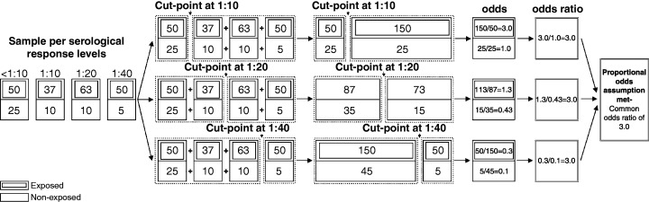
 Schematic illustration of the proportional odds assumptions using serological response levels as example.

The proportional odds model illustrated above can be generalized to several predictors (X ₁, X ₂,…), for example assess the effect of exposure while adjusting for cofounders, namely

In standard practice, the null hypothesis of equal slopes (proportional odds) is tested with the score test for proportional odds. This test is provided by most of the standard statistical packages. A statistically non‐significant test is considered sufficient evidence that the proportional odds assumption was not violated. Because this test is sensitive to sample size and may be significant in cases with minimum deviation from proportionality, some authors recommend plotting the log odds generated by each cut‐point as a complementary analysis for proportionality of odds. ⁷

An illustration with avian and swine influenza

We used existing influenza serological titer data to compare the binary logistic model and the proportional odds models. Titer results were reported as the reciprocal of the highest dilution of serum that inhibited virus‐induced hemagglutination of red blood cells. Data included antibodies against: swine H1N1 and H1N2 viruses among 788 agricultural workers (687 exposed and 87 non‐exposed), avian H1 virus among 73 avian‐exposed veterinarians and 94 non‐avian‐exposed controls, and swine H1N1 viruses among 49 swine confinement workers and 78 non‐swine‐exposed controls. ⁸ , ⁹ , ¹⁰

For the binary logistic model, we adopted the antibody titers of 1:40 as cut‐point for swine influenza viruses ⁸ and 1:10 for avian influenza viruses, ¹ and compute unadjusted odds ratios, as well as odds ratios adjusted for gender alone, and for gender and age. When the standard algorithm for fitting this method was unsuccessful (which happens, for example, when all the exposed subjects have a positive response or when all the non‐exposed are negative), a computer‐intensive algorithm known as the exact method was used.

We used SAS version 9.1 (SAS, Cary, NC, USA) for these statistical analyses. The binary logistic model and the proportional odds model were both fit using Proc Logistic. This procedure employed the standard computing algorithm to fit the model or the exact method, as necessitated by the data. A number of other statistical packages can also be used to fit these models, although not all of them can employ the exact method.

Comparison of theoretical power

We used Whitehead’s formulae for calculations of sample size for the proportional odds model. ¹¹ After rearrangements, the power can be written as:

where  is the standardized normal cumulative distribution function, θ is the expected odds ratio, α is the significance and V is the Fisher’s information.

The proportional odds Fisher’s information, V _p, is defined by:

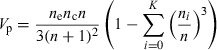where n _e is the exposed group sample, n _c is the non‐exposed group sample, n is the total sample and n _i/n is the hypothetical anticipated proportion of the total sample expected to be in the level i of the ordinal outcome (where i = 0 to K).

Considering the binary logistic as a special case of the proportional odds for a number outcome with only two levels (j = 0 or 1), we can write the Fisher’s information of the binary logistic V _b as:

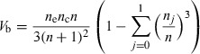When an ordinal data set is dichotomized at a cut‐point L, these two levels formed are the sum of the sample in the level equal or above L and the level lower than L. In this case, we can also represent the binary logistic V _b as:

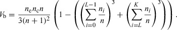To demonstrate that the power of the proportional odds model is greater than the binary logistic, we have to show that:

Considering the significance α to be fixed, and the expected odds ratio θ to be common between models, we can simplify the inequality to:

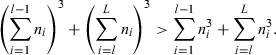Hence, the power for the proportional odds model will always be greater than the power of the binary logistic.

To illustrate, we performed power calculations under a variety of hypothetical scenarios: different odds ratios, number of serological titer levels, sample sizes (at an exposed/non‐expose rate of 1:4) and hypothetical anticipated proportions of subjects per serological titer response. As a relative measure of the performance of these models, we also calculated the relative asymptotic efficiency, ¹² defined as the limit of the sample size ratio required for two methods to reach the same power.

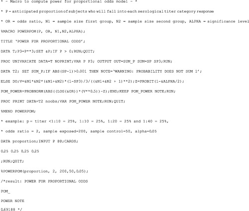
The calculations were the ‘hmisc’ procedure ¹³ of R software (R: A Language and Environment for Statistical Computing, Vienna, Austria). Additionally, a SAS macro for computing the power for the proportional odds model is provided (Table 1).

Table 1.

 A macro for calculation of power for the proportional odds model with SAS

Results

In some data sets, the sparseness of the sample in some titer categories led us to group adjacent categories together. This resulted in acceptable (non‐significant) tests of the proportional odds assumption. The proportional odds model revealed equal or greater evidence of risk factors and outcome associations compared with the binary logistic model (Table 2). This increased evidence is seen in higher chi‐squared values, lower P‐values, and narrower confidence intervals. The odds ratios were very compatible between models.

Table 2.

 Comparison of the proportional odds model and the binary logistic model in analyzing HI serological titer against influenza virus

Data	Population	Outcome	Confounder adjustment	Model	Sample distribution*	Analysis of effect		Exposed vs. non‐exposed
						Wald chi‐squared	P value	Odds ratio	95% confidence interval
1	Swine‐exposed farmers vs. non‐swine‐exposed controls	Swine H1N1	Unadjusted	Binary logistic Proportional odds	682/92 419/140/123/65/22/3/2	4.5 24.4	0.03 <0.01	3.0 3.9	1.1, 8.5 2.3, 6.8
			Gender	Binary logistic Proportional odds	682/92 419/140/123/65/22/5	0.2 5.3	0.65 0.02	1.3 2.0	0.4, 4.0 1.1, 3.6
			Gender and age	Binary logistic Proportional odds	682/92 419/140/123/65/22/5	15.5 7.8	<0.01 <0.01	1.4 2.3	0.5, 4.4 1.3, 4.2
2	Avian‐exposed veterinarians vs. non‐avian‐exposed controls	Avian H1	Unadjusted	Binary logistic Proportional odds	115/52 115/32/13/5/2	16.1 16.0	<0.01 <0.01	4.2 4.0	2.1, 8.4 2.0, 8.0
			Gender	Binary logistic Proportional odds	115/52 115/32/13/5/2	9.6 9.1	<0.01 <0.01	3.2 3.0	1.5, 6.6 1.5, 6.2
			Gender and age	Binary logistic Proportional odds	115/52 115/32/13/5/2	6.6 6.1	0.01 0.01	2.8 2.7	1.3, 6.2 1.2, 5.8
3	Swine‐exposed farmers vs. non‐swine‐exposed controls	Swine H1N2	Unadjusted	Binary logistic Proportional odds	628/146 305/164/159/89/38/14/4/1	8.1 29.6	<0.01 <0.01	3.4 3.6	1.5, 8.1 2.3, 5.7
			Gender	Binary logistic Proportional odds	628/146 305/164/159/89/38/19	1.7 7.1	0.2 <0.01	1.8 2.0	0.7, 4.5 1.2, 3.2
			Gender and age	Binary logistic Proportional odds	628/146 305/164/159/89/38/19	2.0 7.6	0.16 <0.01	1.9 2.0	0.8, 4.8 1.2, 3.3
4	Swine confinement workers vs. non‐swine‐exposed controls	Swine H1N1	Unadjusted	Binary logistic (exact method) Proportional odds	123/4 112/7/4/3/1	NA 11.2	0.04 <0.01	9.0 13.0	1.1, infinity 83.0, 64.5
			Gender	Binary logistic (exact method) Proportional odds	123/4 112/7/4/4	NA 6.9	0.22 <0.01	4.0 8.6	0.5, infinity 1.7, 42.6
			Gender and age	Binary logistic (exact method) Proportional odds	123/4 112/7/4/4	NA 6.4	0.44 0.01	2.5 8.0	0.3, infinity 1.6, 40.2

*Original titer levels <1:10/1:10 – <1:20/1:20 – <1:40/1:40 – <1:80/1:80 – <1:160/1:160 – <1:640/≥1:640. Multivariate POM of data 1 and 3 had levels above ‘1:160 – <1:640’ collapsed to meet POM assumption. The multivariate proportional odds model of data 4 had levels above ‘1:40 – <1:80’ collapsed to meet the proportional odds model assumption. All the presented models meet the proportional odds assumption.

In accordance with the mathematical demonstration, the power calculations illustrate the superiority of the proportional odds model over the binary logistic model. For the same power, the proportional odds require a smaller sample compared with binary logistic model (Figure 2A). A loss of power is noticed when response categories are collapsed (Figure 2B). Changes in hypothetical anticipated proportions of subjects per serological titer response and adoption of different cut‐points were responsible for most of the variation in efficiency (data not shown). The highest relative efficiency of the proportional odds model compared with the binary logistic model was obtained when differences between risk groups are hidden by data dichotomization.

Figure 2.

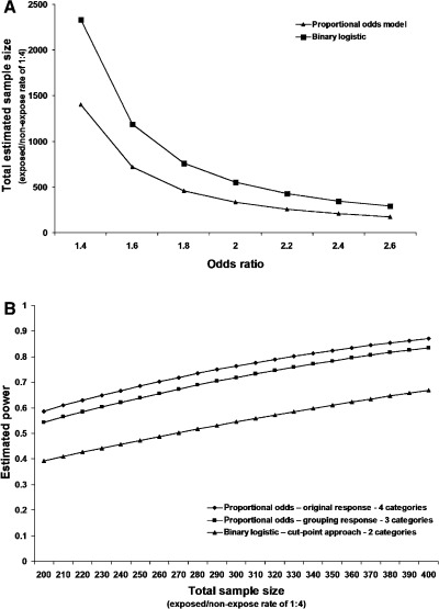
 Panel A – comparison of the estimate sample required for a 80% power, at 5% significance level, with the proportional odds model and the binary model, under an hypothetical anticipated proportion of subjects per serological titer response of <1:10 = 25%, 1:10 = 25%, 1:20 = 25% and 1:40 = 25% (cut‐point of 1:40). Panel B – estimated power, at 5% significance level, for an odds ratio of 2 and hypothetical anticipated proportion of subjects per serological titer response of <1:10 = 25%, 1:10 = 25%, 1:20 = 25% and 1:40 = 25% (proportional odds – original response – four categories); <1:20 = 50%, 1:20 = 25% and 1:40 = 25% (proportional odds – grouping response – three categories); and <1:40 = 75% and 1:40 = 25% (the binary logistic model – cut‐point approach – two categories).

Discussion

In previous studies, we successfully used the proportional odds model, which allowed us, sometimes with a small sample size, to determine risk factors for zoonotic influenza. ⁸ , ⁹ However, our search of the medical literature indicates that the use of the proportional odds model is infrequent. The loss of information observed when ordinal data were grouped into two categories (dichotomization) has been previously reported. ⁷ Recently, in other fields, the superiority of the proportional odds model over the binary logistic model has been explored analytically, yet without comparisons of power. ¹⁴ We provide infectious disease epidemiologists with a more definitive argument.

Our data show that, when the proportional odds assumption is met, the odds ratio calculated with proportional odds will be within the confidence interval of the binary logistic odds ratio. With this observation we raise the question: should we ever dichotomize the ordinal data? Perhaps we should do so when there is strong data supporting that a specific cut‐point provides definitive evidence of protection against infection (e.g. vaccine titer data). Such might justify the loss of power.

The proportional odds model provides an intermediate approach between the cut‐point approach and identification of the actual underlying continuous distribution of serological responses. The interpretation of the proportional odds model is easy because it is similar to the binary logistic, and is unaffected by the direction chosen to model (higher to lower titer vs. lower to higher titer). ¹⁵ However, because of the proportional odds assumption constraint, this model is not appropriate for all data. Brender and Groven demonstrated that the use of POM can lead to invalid results if the proportional odds assumption is violated. ¹⁶ When the proportional odds score test is statistically significant with graphical evidence of non‐proportionality, the investigator may choose to fit a partial proportional odds model. This revised model loosens the constraint that all variables must have proportional odds.

Inferences based on odds ratios are often used in showing a relationship between a predictor and an outcome. In our illustrations, the predictors are environmental exposures and the outcomes are antibody response levels. In other situations, the predictors could be the results of a screening test and the outcomes could be the presence or severity of a disease. Pepe et al. ³ emphasize the use of ROC curves and other classification tools in evaluating the usefulness of screening programs, as seemingly high odds ratios (e.g. in the range of 3–9) may yield very poor classification properties in low‐risk populations. However, these authors discuss only dichotomous outcomes (e.g. presence vs. absence of a disease), which could be analyzed with logistic regression, rather than ordinal outcomes (e.g. severe vs. moderate vs. mild vs. no disease), which lend themselves to the proportional odds model. In fact, as standard ROC analyses are based specifically on dichotomous outcomes, it is not clear how to use them to measure the classification properties of the proportional odds model. Conceptually, a researcher could do a logistic regression analysis based on each possible dichotomization of the outcome and then use ROC criteria to choose the dichotomization which appears to be optimal. However, the theoretical comparisons illustrated in this report imply that even an optimal dichotomization would have less statistical power than inferences based on the proportional odds model.

In summary, these analyses illustrate the advantages of examining the entire spectrum of serological response in an epidemiological study by using the proportional odds method. Because of its superior power, the proportional odds model may identify risk factors that would be otherwise remain undetected by the more often used dichotomization of serologic data. The proportional odds model allows epidemiologists to use smaller sample sizes, which ultimately offers a more economical analysis.

References

- 1. Meijer A, Bosman A, Van De Kamp EE, Wilbrink B, Van Beest Holle Mdu R, Koopmans M. Measurement of antibodies to avian influenza virus A(H7N7) in humans by hemagglutination inhibition test. J Virol Methods 2006; 2:113–120. [DOI] [PubMed] [Google Scholar]
- 2. Olsen CW, Brammer L, Easterday BC et al. Serologic evidence of H1 swine Influenza virus infection in swine farm residents and employees. Emerg Infect Dis 2002; 8:814–819. [DOI] [PMC free article] [PubMed] [Google Scholar]
- 3. Pepe MS, Janes H, Longton G, Leisenring W, Newcomb P. Limitations of the odds ratio in gauging the performance of a diagnostic, prognostic, or screening marker. Am J Epidemiol 2004; 159:882–890. [DOI] [PubMed] [Google Scholar]
- 4. Aitchison J, Silvey SD. The generalization of probit analysis to the case of multiple responses. Biometrika 1957; 2:131–140. [Google Scholar]
- 5. Walker SH, Duncan DB. Estimation of the probability of an event as a function of several independent variables. Biometrika 1967; 54:167–179. [PubMed] [Google Scholar]
- 6. McCullagh P. Regression models for ordinal data. J R Stat Soc Ser B (Methodol) 1980; 42:109–142. [Google Scholar]
- 7. Scott SC, Goldberg MS, Mayo NE. Statistical assessment of ordinal outcomes in comparative studies. J Clin Epidemiol 1997; 50:45–55. [DOI] [PubMed] [Google Scholar]
- 8. Myers KP, Olsen CW, Setterquist SF et al. Are swine workers in the United States at increased risk of infection with zoonotic influenza virus? Clin Infect Dis 2006; 42:14–20. [DOI] [PMC free article] [PubMed] [Google Scholar]
- 9. Ramirez A, Capuano AW, Wellman DA, Lesher KA, Setterquist SF, Gray GC. Preventing zoonotic influenza virus infection. Emerg Infect Dis 2006; 12:996–1000. [DOI] [PMC free article] [PubMed] [Google Scholar]
- 10. Gray GC, McCarthy T, Capuano AW et al. Population‐based Surveillance for Zoonotic Influenza A in Agricultural Workers. Atlanta, GA: International Conference on Emerging Infectious Diseases, 2006. [Google Scholar]
- 11. Whitehead J. Sample size calculations for ordered categorical data. Stat Med 1993; 12:2257–2271. [DOI] [PubMed] [Google Scholar]
- 12. Armstrong BG, Sloan M. Ordinal regression models for epidemiologic data. Am J Epidemiol 1989; 129:191–204. [DOI] [PubMed] [Google Scholar]
- 13. Harrell FE. The hmisc Package. 3.0‐7 edn, http://cran.r‐project.org/doc/packages/Hmisc.pdf , R‐project library, 2005. [Google Scholar]
- 14. Norris CM, Ghali WA, Saunders LD et al. Ordinal regression model and the linear regression model were superior to the logistic regression models. J Clin Epidemiol 2006; 59:448–456. [DOI] [PubMed] [Google Scholar]
- 15. Stokes ME, Davis CS, Koch GG. Categorical Data Analysis using the SAS System. Cary, NC: SAS Institute, 1995. [Google Scholar]
- 16. Bender R, Grouven U. Using binary logistic regression models for ordinal data with non‐proportional odds. J Clin Epidemiol 1998; 51:809–816. [DOI] [PubMed] [Google Scholar]