Morphometric analysis of the C57BL/6J mouse brain

Abstract

Magnetic resonance microscopy (MRM), when used in conjunction with active staining, can produce high-resolution, high-contrast images of the mouse brain. Using MRM, we imaged in situ the fixed, actively stained brains of C57BL/6J mice in order to characterize the neuroanatomical phenotype and produce a digital atlas. The brains were scanned within the cranium vault to preserve the brain morphology, avoid shape distortions, and to allow an unbiased shape analysis. The high-resolution imaging used a T1-weighted scan at 21.5 μm isotropic resolution, and an eight-echo multiecho scan, post-processed to obtain an enhanced T2 image at 43 μm resolution. The two image sets were used to segment the brain into 33 anatomical structures. Volume, area, and shape characteristics were extracted for all segmented brain structures. We also analyzed the variability of volumes, areas and shape characteristics. The coefficient of variation of volume had an average value of 7.0. Average anatomical images of the brain for both the T1 weighted and T2 images were generated, together with an average shape atlas, and a probabilistic atlas for 33 major structures. These atlases, with their associated metadata, will serve as baseline for identifying neuroanatomical phenotypes of additional strains, and mouse models now under study. Our efforts were directed toward creating a baseline for comparison with other mouse strains and models of neurodegenerative diseases.

Introduction

Compared to the large number of volumetric studies on the human brain, relatively few studies address mouse brain morphometry. The brains are traditionally evaluated against histological atlases, based on a single specimen per orientation (Sidman 1971), (Paxinos and Franklin 2000), (Hof, Young et al. 2000). In general slices are coronal and quantitative information is lacking. The difference between in-plane (of the order of micrometers) and inter-plane (~0.2,0.3mm, i.e. of the order of hundreds of micrometers) resolutions, as well as non-uniform slice spacing may make three-dimensional (3D) morphometry very challenging. In contrast, magnetic resonance microscopy (MRM), which can produce images with 10–100 μm isotropic resolution, has proven to be a valuable tool in quantitative brain imaging of the normal mouse, as well as mouse models of human diseases. MRM adds new dimensions to the study of anatomy through tissue contrast based on proton density, T1 and T2 relaxation times, and a true three-dimensional nature. Also MRM has the advantage of being nondestructive, allowing longitudinal studies to be performed on the same live animal in order to monitor brain development, disease progression, or treatment response. When imaging fixed specimens, the spatial relationships and connections among brain structures are preserved, in contrast with histology, where distortions can occur in slices.

Digital brain atlases based on MRM offer the possibility of evaluating anatomy along arbitrary axes, observing spatial relationships, quantifying the volumes of segmented structures, and reconstructing shapes in 3D. These attributes make MRM a modality of choice for assessing the effect of genetic manipulation on the anatomical phenotype. Prior to assessing anatomical changes in animal models of disease, it is important to assess the range of normal variability.

A number of recent studies have provided digital atlases of the mouse brain, some incorporating estimates of anatomical variability. For example, (MacKenzie-Graham, Lee et al. 2004) have incorporated into their Mouse Atlas Project MRM images with 100 μm resolution, along with blockface imaging, classical histology, and immunohistochemistry. A qualitative evaluation of datasets is possible, but their segmentations have not been subjected to quantitative variability analysis. A brain atlas incorporating estimates of anatomical variability, at 60 μm resolution, was published for a population of 129S1/SvImJ mice (Kovacevic, Henderson et al. 2005). Anatomic segmentation was achieved through registration of individual brains to the manually labeled average brain. Local variability was estimated via the magnitude of the deformation fields. A similar technique has been employed by the same group to compare three strains of mice: 129S1/SvImJ (that provided the initial segmentation template), C57BL/6, and CD1 (Chen, Kovacevic et al. 2006). A database including a minimum deformation and a probabilistic atlas for the C57BL/6 brain, at 47μm resolution, has been proposed by Ma and colleagues (Ma, Hof et al. 2005). This atlas includes 20 structures, segmented based on registration to a manually labeled reference brain. All these MRM-based data on brain variability rely on specimens imaged after removal from the cranium, therefore prone to distortion or damage, particularly in regions like the olfactory bulb, or paraflocculus of the cerebellum.

In this work, we performed a morphometric analysis of the C57BL/6J mouse brain, based on MRM of actively stained brains in situ, i.e. within the cranium, to eliminate the possibility of damage or distortion of the brain. Imaging protocols included a T1-weighted scan at 21.5 μm resolution, and an eight-echo T2 scan at 43 μm that take advantage of the different tissue contrast mechanisms associated with the two different types of scans. Data from both imaging scans are input to a segmentation algorithm that uses Markov random field (MRF) modeling of contextual priors (Ali, Dale et al. 2005). The actively stained mouse brain is thus automatically segmented into 33 major structures.

A key feature of this work is that automated segmentation allowed accurate morphometry (volume, area), as well as unbiased shape analysis. A surface-based shape analysis was performed for the segmented structures at global and local scale. One shape metric is the fractal dimension (FD), which has been used to describe abnormalities of cortical morphology in patients with neurologic disorders (Bullmore, Brammer et al. 1994) and proposed as a measure of differences in the complexity of MRI boundaries or irregularities of the outline. Here we employed the fractal dimension to characterize the complexity of shape for the segmented structures. Besides FD, the variability in shape was also characterized using distance metrics, such as the Hausdorff distances (Preparata and Shamos 1985). While the Hausdorff and the mean distances characterized the global shape, local shape changes were illustrated using root mean square distances between corresponding vertices on the surfaces of these structures.

Average images for the T1 and T2 imaging protocols, as well as an average shape atlas and a probabilistic atlas of the mouse brain were also constructed from the data. These three atlases of the wild type brain, with their associated metadata, will serve as baseline for identifying neuroanatomical phenotypes of other strains and disease models. The atlases and original datasets are offered online as part of the Mouse Bioinformatics Imaging Research Network (MBIRN) (Martone, Gupta et al. 2004).

Materials and Methods

Animal preparation

Six adult C57BL/6J mice, (The Jackson Laboratory, Bar Harbor, ME, USA), about 9 weeks old, were used in this study. All experiments were conducted in accordance with NIH guidelines, using protocols approved by the Duke University Institutional Animal Care and Use Committee. The mice were anesthetized with 100 mg/kg pentobarbital (i.p.) and then transcardially perfusion fixed, first with a flush of a mixture of 0.9% saline and ProHance (Bracco Diagnostics, Princeton, NJ), in a volume ratio of 1 part ProHance to 10 parts total, followed by perfusion with Prohance mixed into buffered formalin (10% phosphate buffered formalin, SF100-20, Fisher Scientific, Chicago, IL — equivalent to 4% formaldehyde), in a volume ratio of 1 part ProHance to 10 parts total (Johnson, Cofer et al. 2002). The heads were stored overnight in formalin, and then trimmed to remove lower jaw and muscle before being scanned. The brains were left in the cranium to avoid distortions or damage to the tissue associated with excision from the cranium.

Imaging protocols

The specimens were placed in fomblin-filled tubes, scanned on a 9.4 T, 8.9 cm vertical bore Oxford magnet with a General Electric (GE Healthcare, Milwaukee, WI) EXCITE console (Epic 11.0), using a 12 mm diameter solenoid coil. Two scan protocols were used to image each brain, producing registered datasets, since the specimens were left in the same position in the magnet from scan to scan. The first protocol consisted of a 3D T1-weighted spin warp sequence with echo time (TE) 5.1 ms, repetition time (TR) 50 ms, 62.5 kHz bandwidth, field of view (FOV) of 11×11×22 mm. For the T1-weighted array, the Fourier volume was asymmetrically filled with 384×384×768 samples. The asymmetric sampling was extended along all three axes to the Nyquist limit corresponding to 21.5 μm. The receiver gain was increased at the periphery of Fourier space to provide an expanded dynamic range and effectively weight these higher frequencies. The higher frequency points on the opposite extremes of the Fourier volume were zero-filled to produce 512×512×1024 image arrays. The method allows acquisition of high-resolution images with much reduced scan time (Johnson et al, 2006, submitted). The second imaging protocol consisted of a 3D Carr-Purcell-Meiboom-Gill (CPMG) sequence with 8 echoes, post-processed using MEFIC, and resulting in a T2 dataset with increased contrast and signal-to-noise-ratio (SNR) (Sharief and Johnson 2006). The parameters for this protocol were: interecho spacing 7 ms, 8 echoes, TR 400 ms, 62.5 kHz bandwidth, FOV 11×11×22 mm, matrix size 256×256×512 pixels, yielding an isotropic resolution of 43 μm. These sequences used the same asymmetric Fourier sampling with expanded dynamic range described above, filling a 192×192×512 array with subsequent zero-filling on one side (25%) of each phase encoding axis. The scan times were 2 hours 7 minutes for the T1 protocol, and 4 hours 15 minutes for the T2 protocol.

Image preprocessing

An algorithm based on mathematical morphology (Hohne and Hanson 1992) (Badea, Kostopoulos et al. 2003) was used to isolate the brain from surrounding cranium and tissues, a process termed skull-stripping in the human brain segmentation literature. The algorithm starts with smoothing, followed by thresholding and erosions. Region growing starts then from a seed point automatically selected in the center of the volume. Voxels with values between fixed thresholds and connected to the initial region are added to the brain mask. Dilation is applied at the end on the brain mask, for the same number of times erosion has been applied. Following skull-stripping, the voxel values were intensity normalized to the same global range (0: 32768) and histogram matched. The brains were then brought into a common same space using an affine (12 parameters) transform and the Image Registration Toolkit (ITK) (Rueckert, Frangi et al. 2003).

In the process of segmentation each brain voxel was assigned a label from one of the 33 predetermined labels. The automatic segmentation used a combination of spatial and contextual priors, and the grayscale intensity features from T1-weighted and T2-weighted images (Ali, Dale et al. 2005). The segmentation has been validated in the present study by computing the percentage voxel overlap between the anatomical structures that were segmented automatically and those segmented manually. As a second test, the segmentation has been validated comparing the results with those obtained from an atlas-based segmentation, based solely on registration with a labeled reference brain. For the later case, one brain selected as the reference, manually labeled, was registered first using an affine, and then a non-rigid transform (Rueckert, Sonoda et al. 1999) to each of the other brains. The voxel labels were subsequently mapped in the native space of the individual brains, according to the same transforms. The percentage voxel overlap was computed for both segmentation methods for the remaining five brains (excluding the reference), and their corresponding manual labels.

For shape analysis of the segmented structures, each structure was analyzed separately after thresholding it out of the labeled brain volume. Corresponding label volumes from all six brains were registered with an affine transform, in order to remove sources of variability that can arise from changes in position, orientation, or scale. After registration the volumes were binarized, using a threshold value of 50% of the original gray value, assigned to the particular label. BRAINSUITE (Shattuck and Leahy 2002) was used to generate isosurfaces and triangulated meshes for the segmented structures. These meshes characterizing the boundaries of 33 major neuroanatomical structures were subsequently used for shape analysis using software written in MATLAB (The Mathworks, Natick, MA).

Morphometry

Absolute volumes for individual segmented structures and the whole brain were calculated using the number of voxels, and multiplying this number by the voxel volume. Surface areas were calculated by summing the areas of individual triangles of the surface mesh of each structure.

For global measure of shape we used the fractal dimension (FD), which was proposed as a measure of shape complexity, and reflects the rate at which the volume of an object increases as the scale of measurement is reduced (Barabasi and Stanley 1995). The FD was calculated using the box-counting method (Barabasi and Stanley 1995), from the slope of the log-log plot that relates the number of boxes necessary to cover the volume of interest to their size. If N_b (l_b ) was the number of boxes with size l_b needed to completely cover the structure the fractal dimension was calculated as:

$$FD=-\underset{l_b\to 0}{lim}\frac{{log}_{10}{N}_b(l_b)}{{log}_{10}{l}_b}$$

After registering the segmented structures to a common space, correspondence between meshes was established based on the minimum distance between pairs of vertices. The mean shapes for individual structures were generated using the linear average of the corresponding (closest) vertices from each of the brains.

The degree of mismatch between each shape and the average shape for the group was measured using the Hausdorff distance (HD) (http://www.nist.gov/dads/HTML/hausdorffdst.html). HD was calculated as the maximum of minimum distances between corresponding points (r_i and r_j) from two shapes (S₁ and S₂), computed forward and backward, according to (Huttenlocher, Klanderman et al. 1993).

$$HD(S_1,S_2)=max(h(S_1,S_2),h(S_2,S_1)),\hspace{0.17em}\hspace{0.17em}\hspace{0.17em}\text{where\hspace{0.17em}}h(S_1,S_2)=\underset{r_i\in S_1}{max}\underset{r_j\in S_2}{min}\Vert r_i-r_j\Vert$$

The usefulness of the HD metric results from its interpretation as a global distance between shapes. To analyze variations in local shape, distance maps were used to pseudocolor the surfaces of segmented structures. Specifically, elementary patches that make the average structures surfaces were colored in accordance to the root mean square (RMS) distance between corresponding vertices of the original meshes and those of the average shape. The mean value of the local distances was used as a global shape characteristic.

In summary, the metrics used to assess the variability between the 6 brains were the volumes of the segmented structures, and the associated coefficient of variation of volume, surface areas, fractal dimensions, Hausdorff and mean distances, and RMS distance maps.

Atlasing

The final phase of our study was to use the segmented brains imaged in situ to form an atlas. The atlas comprises: 1) average brain images for the T1-weighted and T2 datasets, 2) an average shape atlas, and 3) a probabilistic atlas.

We constructed an average labeled brain, based on the individually segmented brains (Ashburner 2000) (Rohlfing, Brandt et al. 2001). The average shape image was found after an affine transform of the segmented datasets, followed by a series of nonlinear transforms, performed using AIR 5.2 (Woods, Grafton et al. 1998). The affine transform mapped the original images, T1-weighted and T2, to a reference image, to generate an initial average. The algorithm proceeded to several nonrigid registrations of the original images to the previous iteration’s result, to produce at each step a new “average image”. In this average image each voxel was assigned the label that was most frequently found at one location in all the brains. For example, if at one particular voxel location, the label assigned is hippocampus in 5 brains, and ventricle in another brain, that voxel will be labeled as hippocampus in the average shape brain.

The construction of the average shape atlas involved the use of the nearest neighbor interpolation when reslicing the label volumes to match the atlas space. The same transforms used to bring the segmented shapes into registration were used for the intensity normalized grayscale images, in order to construct average grayscale volume for the T1-weighted and T2 datasets.

For each structure, for example l, segmented, and at each voxel location r⃗ (x, y, z), in the space of the N co-registered brains, the probability can be calculated as:

$$p_{l,\overrightarrow{r}}=\frac{\sum _{i=1}^N{\delta }_{(l,{\mathit{label}}_{i,\overrightarrow{r}})}}{N}\bullet 100\hspace{0.17em}(\%),\hspace{0.17em}\text{where\hspace{0.17em}}\delta \hspace{0.17em}\text{is\hspace{0.17em}Kronecker's\hspace{0.17em}delta\hspace{0.17em}function}.$$

To construct a probabilistic atlas, we used the frequency of occurrence of a particular label at a certain location (Ma, Hof et al. 2005). A voxel value is given by the number of times is has been assigned that label over the set of six brains, in percentage. The probabilistic atlas can be thresholded so that at a threshold of 0%, an absolute majority is required for a voxel to be labeled. At 50%, at least half of the labels have to be in agreement in order for the voxel to be labeled. At 100%, all of the labels have to agree for the voxel to be labeled. Otherwise the voxel label is considered undecided.

Results

The two imaging protocols used in this study of the C57BL/6J mouse brain (T1-weighted and T2) provided complementary information, which allowed the identification of 33 major neuroanatomical structures. A qualitative comparison of the two different contrasts is made in Figure 1, which shows cross-sections in the three cardinal planes through the T1-weighted image (A), MEFIC processed T2 image (B), as well as 24 anatomical structures (C) for one specimen. Table 1 shows the complete list of segmented structures, which includes the ventricular system, white matter tracts, large gray matter structures, as well as selected groups of nuclei that were identifiable in the T2 image. Some of these labels were not included, to the best of our knowledge, in previous MRM atlases (MacKenzie-Graham, Lee et al. 2004; Ma, Hof et al. 2005) (Kovacevic, Henderson et al. 2005) — deep mesencephalic reticular nucleus and red nucleus (DpMe), anterior pretectal nucleus (APT), thalamic nuclei including ventral posterior and lateral thalamic nuclei (VT), lateral dorsal nucleus (LD), geniculate bodies (Gen), trigeminal tract, pons, cochlear nucleus, and lateral lemniscus.

Figure 1.

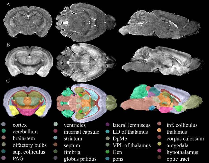
Cross-sections through the T1-weighted image (A), MEFIC processed T2 image (B), and segmented volumes (C) of the same specimen. The T1-weighted image has a 21.5 μm resolution and presents a different contrast than the T2 image at 43 μm resolution, where thalamic nuclei could be identified. The combined information from both image protocols led to the identification of 33 structures (C).

Table 1.

Segmented structures, the abbreviations used and their segmentation accuracy, evaluated by means of percentage voxel overlap with the manual labels.

Label	Abbreviation	Voxel overlap (±SD) %	Label	Abbreviation	Voxel overlap (±SD) %
Accumbens nucleus	Acb	87.32 (0.02)	Internal Capsule	ic	76.39 (0.05)
Amygdala	Amy	91.10 (0.01)	Interpeduncular Nucleus	IP	80.58 (0.08)
Anterior Commisure	ac	76.20 (0.04)	Lateral Lemniscus	ll	83.32 (0.03)
Anterior Pretectal Nucleus	APT	83.82 (0.05)	Laterodorsal nucleus of thalamus	LD	86.44 (0.04)
Brainstem	BS	93.10 (0.02)	Olfactory Bulbs	OLF	91.76 (0.03)
Cerebellum	Cb	95.49 (0.01)	Optic Tract	ot	75.41 (0.08)
Cerebral Cortex	Cx	93.56 (0.01)	Periaqueductal gray	PAG	85.05 (0.01)
Cerebral Peduncle	cp	68.90 (0.05)	Pontine nuclei	Pn	76.92 (0.07)
Cochlear Nuclei	Co	77.28 (0.05)	Septum	SX	87.06 (0.03)
Corpus Callosum	cc	76.48 (0.01)	Spinal Trigeminal Tract	sp5	67.30 (0.04)
Deep Mesencephalic Nucleusa	DpMe	92.05 (0.01)	Striatum	Str	93.96 (0.01)
Fimbria	fi	84.55 (0.02)	Substantia Nigra	SN	85.55 (0.02)
Geniculate complex	Gen	81.51 (0.02)	Superior Colliculus	SC	91.16 (0.01)
Globus Palidus	GP	87.18 (0.03)	Thalamus	TH	92.20 (0.01)
Hippocampus	HC	91.83 (0.01)	Ventral nuclei of thalamusb	VT	84.95 (0.03)
Hypothalamus	Hyp	93.28 (0.01)	Ventricular system	VS	76.11 (0.03)
Inferior Colliculus	IC	87.77 (0.02)

^aDpMe were segmented together with the red nucleus

^bVT include the ventral posterolateral, ventral posteromedial, ventrolateral, and ventral anterior nucleus

Several anatomical structures were hard to distinguish based on one single protocol, but could be segmented based on combined information from both types of images. For example, only in the T2 images the geniculate bodies (Gen), the latero-dorsal nucleus of the thalamus (LD), and ventral nuclei of the thalamus (VT, which include the postero lateral nucleus or VPL), as well as the deep mesencephalic nucleus and red nucleus (DpMe) became apparent, while the lateral lemniscus (ll) and cortical layers were seen in the T2 images with good contrast (Figure 2). On the other hand, the higher resolution T1-weighted images present a good definition of hippocampal layers (Figure 2, row A) and thin white matter tracts like fimbria.

Figure 2.

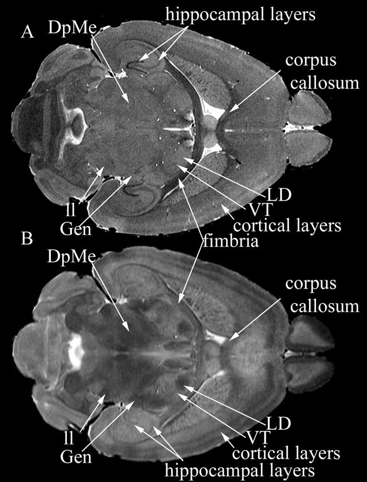
Comparison of the contrasts characteristic to T1-weighted (A) and MEFIC processed T2 images (B). The T1-weighted image allowed discrimination of hippocampal layers, cortical layers, and thin white matter tracts like fimbria and corpus callosum. In the T2 image, the deep mesencephalic reticular nucleus and red nucleus (DpMe) became apparent, as well as the lateral lemniscus (ll), while the cortical layers were seen with greater contrast. Among the thalamic nuclei the geniculate nuclei (Gen), the latero-dorsal nucleus (LD), and ventral postero-lateral nucleus of the thalamus (VPL) could be identified.

We validated the Markov random field (MRF) segmentation method, and found it to perform consistently, by computing the percentage voxel overlap between the automatically and the manually generated labels (Table 1). The average value for the percentage voxel overlap was 85.72%. The percentage voxel overlap was better than 90% for structures like cerebellum (95.49%), striatum (93.96%), cerebral cortex (93.56%), brainstem (93.10%), even smaller structures like DpMe (92.05%), while at the other end of the scale were the ventricles (76.11%), and white matter tracts like the optic tract (75.41%), cerebral peduncle (68.9%) and trigeminal tract (67.30%). Also the MRF segmentation has been found to perform well when compared with an atlas based segmentation, as illustrated in Figure 3. The average voxel overlap in the case of MRF based segmentation (disregarding the reference brain) is 85.0±7.5%, while for the atlas based segmentation is only 72.7 ±15.1%, the difference being significant for many of the segmented structures, marked with asterisks in Figure 3.

Figure 3.

Segmentation accuracy in the case of multispectral (MRF) segmentation and registration based segmentation (nlin) as reflected by the percentage voxel overlap. The average voxel overlap in the case of MRF segmentation is 85.0±7.5%, while for the purely registration based segmentation is 72.7 ±15.1%, the difference is significant where indicated with asterisks.

We calculated traditional morphometric parameters to characterize gross neuroanatomical structures for a normal population of young adult C57BL/6J mice. These parameters include the volumes of anatomical structures (Figure 4), with the associated coefficients of variation (Figure 5), as well as the surface area for these structures (Figure 6). To the best of our knowledge, variability in several of these structures has not been previously reported based on MRM studies, e.g. for the deep mesencephalic nucleus and red nucleus (DpMe), ventral thalamic nuclei (VT) including ventral posterior and lateral thalamic nuclei (VPL), anterior pretectal nucleus (APT), lateral dorsal nucleus (LD), geniculate body (Gen), trigeminal tract, pons, cochlear nucleus, substantia nigra, and lateral lemniscus. The whole brain averaged 508.91±23.42 mm³. Among the largest structures segmented were the cerebral cortex (169.61±8.88 mm³) and brainstem (79.19±4.03 mm³), while the smallest were the laterodorsal nucleus of the thalamus (0.43±0.03 mm³) and the interpeduncular nucleus (0.41±0.07 mm³).

Figure 4.

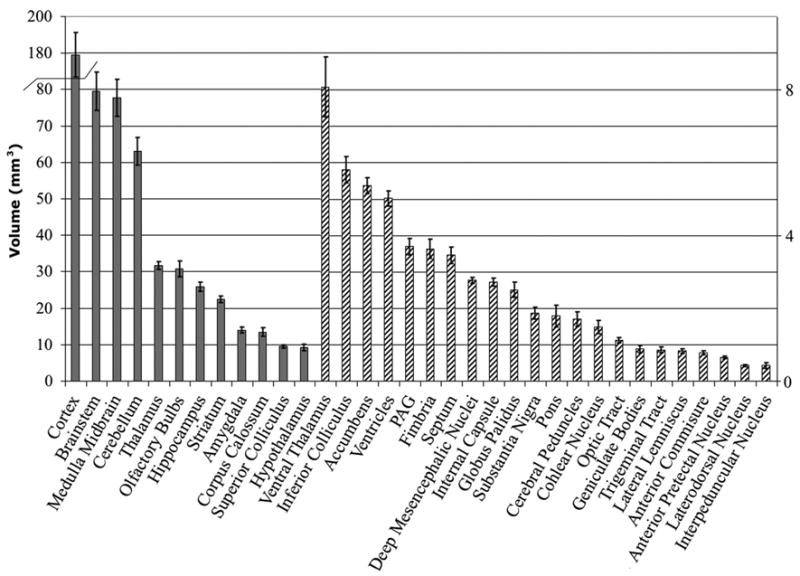
Volume measurements for the segmented structures. Large structures are represented on the left axis using solid colors, smaller structures are represented in the right axis using a striped pattern.

Figure 5.

Volume coefficient of variation describes the variability of the segmented structures independently of their absolute size, which ranged from 19.8% for the interpeduncular nucleus (IP), to 3.3% for thalamus, and 2.9% for the deep mesencephalic reticular nucleus and red nucleus (DpMe).

Figure 6.

Area measurements for the segmented structures ranged from 348.48±3.31mm² for cortex (not shown), followed by the rest of brainstem and corpus callosum (125 ±1.60, and 120.43±6.16mm²), to 1.56±0.12 for LD (latero-dorsal nucleus of the thalamus) and 1.40 ±0.07 mm² for interpeduncular nucleus.

A comparison of the measured volumes in the current study and other published data (Ma, Hof et al. 2005) indicates good agreement in general, particularly for internal structures such as hippocampus (25.75±1.04 mm³ versus 25.71±1.08 mm³), corpus callosum (14.43±1.72 mm³ versus 14.83± 1.71 mm³), internal capsule (2.74±0.10 mm³ versus 2.57±0.15 mm³), but we obtained larger volumes for the brainstem 79.19±4.03 mm³, versus 56.91±5.47 mm³), cerebellum (63.33±2.94 mm³ versus 54.22±2.51 mm³ ), olfactory bulbs (30.96±1.78 mm³ versus 22.94±1.55 mm³) and ventricles (4.80±0.40 mm³ versus 1.52±0.47 mm³). All structures in the latter category are among those likely to be damaged in the process of extraction from the cranium.

To compare the volume variability of these structures, while compensating for differences in their absolute size, the coefficient of variation of volume was calculated. These results are summarized in Figure 5. Several structures were characterized by very low coefficients of variation, less than 5%, indicating a high consistency of the segmentation and low natural variability of the volumes. The structures characterized by low volume variation coefficients include: DpMe (2.9%), thalamus (3.3%), superior colliculus (4.0%), nucleus accumbens (4.0%), striatum (4.1%), internal capsule (4.2%), ventricles (4.2%), hippocampus (4.9%), and pretectal nucleus (5.0%). At the other end of the scale were structures with a large coefficient of variation, e.g. greater than 10% including cerebral peduncle (11.4%), cochlear nucleus, (12.2%), pons (16.8%) and interpeduncular nucleus (19.8%). A comparison of the data in the current manuscript against published data (Ma, Hof et al. 2005), for a subgroup of common structures, indicate that the volume coefficient of variation values are comparable for most structures but smaller for ventricles (8.3% versus 30.9%), brainstem (5.1% versus 9.6%), and olfactory bulbs (5.7 versus 6.8%), with a reverse trend though for structures like hypothalamus (7.6% versus 3.8%), globus pallidus (7.0% versus 4.3%) and central gray (5.5% versus 3.5%).

Surface area measurements were done for all the segmented structures and the results are summarized in Figure 6. These ranged from 348.48±3.31 mm² for cerebral cortex (not included in the graph), 120.43±6.16 mm² for corpus callosum, to 110.3 ±1.17 mm² for brainstem, to 1.56±0.12mm² for latero-dorsal nucleus of thalamus, and 1.40±0.07 mm² for interpeduncular nucleus.

In addition to the traditional morphometric parameters, we used metrics from computational anatomy that reflect shape characteristics. These were extracted following an affine registration of structures of the same type from the six brains. This registration process removed global differences in size and allowed the comparison of shapes. Shape can be characterized globally using parameters like the fractal dimension (Figure 7) and the Hausdorff distance (Figure 8). The fractal dimension (FD), measured using a box-counting method, indicated higher values for cerebral cortex (2.37±0.01), and also for tracts like the corpus callosum (1.92±0.01). Lower values were obtained for interpeduncular nucleus (1.3±0.01), while the ventricles had midrange values (1.63±0.01). The Hausdorff distance was used as a measure of shape variability. It was based on the distance between sets of points representing the structure’s boundaries in different specimens, and was calculated between each shape and the average. Since the Hausdorff distance could be affected by noise in the mesh representation, the mean distance (MD) was used as well. These distance values are shown in Figure 8, and they range from: 0.77±0.20 mm for HD and 0.11±0.02 mm for MD for cortex, to 0.04 ±0.01 mm for HD and 0.02±0.01 for MD for latero-dorsal nucleus of thalamus (one voxel). The mean distance between segmented structures and their average shape had a average value of 0.044±0.01 mm, and indicated a larger discrepancy for large structures, like cortex and brainstem, and smaller values for small nuclei like deep mesencephalic nuclei and red nucleus, geniculate body, interpeduncular, and anterior pretectal nucleus.

Figure 7.

Fractal dimension (FD) estimates for the segmented structures. FD is a shape characteristic that measures the degree of shape complexity, and it ranged from 2.38 for cortex to 1.24 for LD.

Figure 8.

Shape variability expressed in terms of mean distances (MD) between the shapes or Hausdorff distances (HD). The largest values are obtained for large structures like cortex (HD: 0.77 mm, MD: 0.11 mm), thalamus, and some white matter tracts like corpus callosum, optic tract, and anterior commissure, while the smallest values are obtained for the latero-dorsal thalamic nuclei (LD) (HD: 0.04 mm, MD: 0.02 mm).

For a local analysis of the shape variability, distance maps were constructed for each of the segmented structures. A few examples of distance maps distributions are shown for selected structures in Figure 9. For structures like the cortex, corpus callosum, and striatum the distribution of distance values is strongly skewed to the left, suggesting that most distance values are in the smaller range. A compact structure like corpus callosum appears to have higher shape variability (297 μm), compared to striatum (139 μm) and hippocampus (139 μm). The distance distribution includes more values in the higher range for the cerebellum. The distance values appear relatively uniformly distributed on the surfaces of anatomical structures. However the maxima tend to be localized in specific areas for the ventricles, i.e. the curvature at half distance between the dorsal and ventral aspect of the lateral ventricles.

Figure 9.

Examples of local shape characteristics evaluated using mesh representations of segmented structures. The mean shapes are pseudo-colored according to distance maps; each vertex is assigned a value equal the root mean square distance (RMS). Under each shape is represented the distance distribution, along with the minimum and maximum RMS values.

Average shape and probabilistic atlases (Figure 10) were constructed based on the segmented images. The 6 T1-weighted and T2-weighted datasets, of which sample images are shown in (Figure 10, upper row), were used to create average images for each acquisition protocol (Figure 10, middle row) based on the registration transforms determined from the labeled datasets. The average images present a higher signal to noise ratio compared to images of individual specimen, enhancing features common to all brains but blurring eventually small structures or edges. The average shape atlas was built using a succession of affine and nonlinear registrations of the labeled sets (Figure 10, left lower row). The number of labels at a particular voxel location was used to build a probabilistic atlas (Figure 10, right lower row). As expected, the low probability areas were found at the border of structures and in regions where small structures are in close vicinity. The probabilistic atlas can be generated at different thresholds of probability values to give insight into locations of areas of greater variability, or poor overlap between the labels assigned in the six brain.

Figure 10.

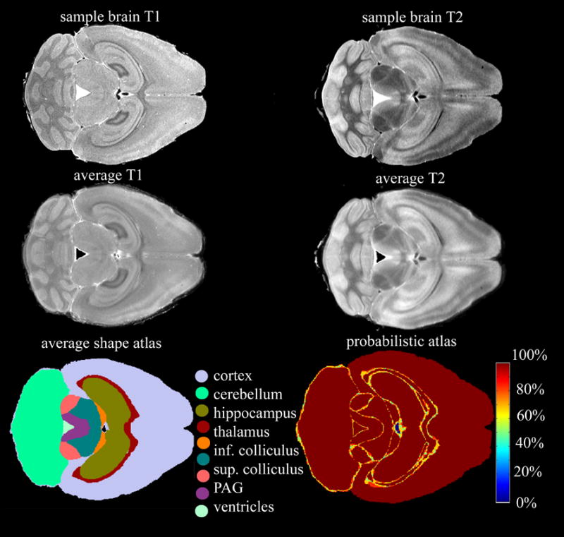
T1-weighted and T2 images (top row) are used to create average brains (middle row) and atlases (bottom row). The average shape atlas (lower row, left) is built based on nonlinear registration of the labeled datasets. The number of labels at a particular voxel location is used to build a probabilistic atlas (lower row, right). A 100% value assigned to a voxel indicates that all labels, in all brains, at that particular location are in agreement, an 80% value indicates that a minimum of 80% labels assigned at that particular location are in agreement, and so on. The low probability areas are found at the border of structures, and in regions where small structures are in close vicinity.

Discussion

The evaluation of neuroanatomical phenotypes for mouse models of disease requires a baseline for comparison, such as an atlas. However, traditional atlases lack quantitative information. Using MRM we generated a probabilistic atlas of the C57BL/6 mouse brain that incorporates quantitative information on 33 major structures. The atlas consists of dual MR images (T1, T2) of the average brain, an average shape and a probabilistic representation. Our approach presents several advantages in characterizing the morphometry of the mouse brain. First, the specimens were left in the cranium to avoid sources of variability resulting from removal of brain from cranium, such as tissue damage and distortion. Second, enhanced tissue contrast was achieved in two ways: a) the use of an MR contrast agent (ProHance), and b) a MEFIC method (Sharief and Johnson 2006). Third, a dual imaging protocol was used to produce co-registered 3D images, which served as input to automated segmentation software. These datasets allowed the segmentation of major neuro-anatomical structures, several small groups of nuclei and the observation of cellular layers.

Previous work has focused on measuring regional volumes (Kovacevic, Henderson et al. 2005) and surfaces (Ma, Hof et al. 2005) of subregions in the brain based on manual and registration-based segmentation. In the present study, a segmentation protocol based on multispectral MR data was used to identify 33 structures from actively stained brain specimens. Because of its automated nature the segmentation method increased objectivity when determining the extent of individual anatomical structures, compared to manual segmentation. Previously the segmentation was evaluated for consistency in the case of formalin fixed mouse brains imaged at 90 μm isotropic resolution (Ali, Dale et al. 2005) and found to have accuracy comparable to studies on the human brain. We found the segmentation to be even more accurate in the present study, and we attribute this to several factors including the enhanced tissue contrast, the higher resolution of the T1-weighted and T2 images of the brains, and the fact that the brains were imaged in situ.

The results of automated segmentation were used to extract accurate and unbiased shape information, in addition to conventional morphometry. Morphometric parameters for some of the structures identified here have not been previously reported in MRM-based studies (Ma, Hof et al. 2005) (Kovacevic, Henderson et al. 2005) (MacKenzie-Graham, Lee et al. 2004). These structures include: deep mesencephalic and red nuclei (DpMe), thalamic nuclei including ventral posterior and lateral thalamic nuclei (VPL), lateral dorsal nucleus (LD), geniculate bodies (Gen), anterior pretectal nucleus (APT), trigeminal tract, pons, cochlear nucleus, and lateral lemniscus.

Our results suggest that scanning the brains in the cranium improved the accuracy of volume estimation, and led to an unbiased appreciation of shape properties. For example, after normalizing for brain weight, our results indicated larger values for the ventricles compared to those reported in previous studies done with the specimens scanned outside the cranium (Ma, Hof et al. 2005) (Chen, Kovacevic et al. 2006). We believe that in the course of preparation for imaging, in brains removed from the cranium the ventricles (which have no intrinsic resiliency) are inadvertently compressed. Also, during extraction from the cranium many structures, such as the brainstem, cerebellum and olfactory bulbs, can be damaged or distorted, and our results indicate that leaving the brains in the cranium reduces variability in these structures. A critical advantage of the in situ MRM-based atlas that we describe is the preservation of the anatomical integrity of the brain.

Neuroanatomical phenotyping is usually based on volumetric characteristics of individually, often manually segmented structures. While this is adequate when the structures of interest are known a priori or have gross deviation, detecting unexpected or subtle phenotypes requires more advanced techniques. Among these, whole brain automated segmentation, as used in this manuscript can be useful for detecting subtle changes in anatomical structures. Besides volume changes, subtle changes in morphometry can be detected based on shape analysis. We present tools, which offer the possibility to visualize and localize areas with prominent differences in shape. Statistical tools for shape analysis would be beneficial in identifying and quantifying possible changes between mice of different strains or in mouse models of disease.

Such an example of a mouse model for neurological and psychiatric conditions is the Reeler mouse. Morphometric changes for individual structures were identified in global parameters such as volumes, area, and fractal dimension, as well as local shape changes, in the hippocampi and ventricles of the Reeler mouse (Badea, Nicholls et al. 2007). A further step would be to use these morphometric parameters in an approach to characterize the development and maturation of the mouse brain, where previous diffusion tensor imaging studies such as (Mori, Itoh et al. 2001), eventually combined with deformation field analysis, showed patterns of evolution in cortical organization in normal populations (Verma, Mori et al. 2005), and great potential for applicability to transgenic and knockout models of cortical dysfunction.

The utility of probabilistic atlases, which are based on multiple datasets, is that they capture the neuroanatomical variability within a reference population, and have the potential to identify an abnormal individual or group that deviates from the reference average. In contrast with other approaches, the shape atlas was constructed based on the labels and not on a standard or reference brain based on the registration of gray volumes. This iterative process of shape averaging provided a “shape centroid” and a minimum deformation from each of the individual brains.

This approach adds new data on several anatomical structures, including traditional measures such as volume and area, and their variability, but also shape information to existing MRM-based information on the mouse brain. Our contribution adds metrics from computational anatomy to describe the neuroanatomical phenotype of a widely used mouse strain, the C57BL/6J. These data on the normal population, with its estimates of variability, can serve as a reference for comparison of morphometric parameters for potential outliers or to mouse models of neurodegenerative diseases. Global changes can be identified in parameters such as volumes, area, and fractal dimension, while more subtle local shape changes can be identified for individual structures.

In the future we anticipate that more and more investigators will rely on comparing in vivo MR atlases of anatomy with atlases based on fixed specimens imaged in situ, a promising start being a study (Nieman, Flenniken et al. 2006) where measures from in vivo MRI were compared with ex vivo, in situ MRI, and additionally microCT data are used to identify phenotypes in the brain and skull of a mutant mouse. Similarly, (Benveniste, Ma et al. 2007) used an atlas of the ex vivo, ex situ mouse brain to drive the segmentation of an in vivo mouse brain.

References

- Ali AA, Dale AM, et al. Automated segmentation of neuroanatomical structures in multispectral MR microscopy of the mouse brain. NeuroImage. 2005;27(2):425–435. doi: 10.1016/j.neuroimage.2005.04.017. [DOI] [PubMed] [Google Scholar]
- Ashburner J. Computational Neuroanatomy. London: University College; 2000. [Google Scholar]
- Badea A, Kostopoulos GK, et al. Surface visualization of electromagnetic brain activity. J Neurosci Methods. 2003;127(2):137–47. doi: 10.1016/s0165-0270(03)00100-6. [DOI] [PubMed] [Google Scholar]
- Badea A, Nicholls PJ, et al. Neuroanatomical phenotypes in the reeler mouse. Neuroimage. 2007;34(4):1363–74. doi: 10.1016/j.neuroimage.2006.09.053. [DOI] [PMC free article] [PubMed] [Google Scholar]
- Barabasi AL, Stanley HE. Fractal Concepts in Surface Growth. Cambridge: Cambridge University Press; 1995. [Google Scholar]
- Benveniste H, Ma Y, et al. Anatomical and functional phenotyping of mice models of Alzheimer’s disease by MR microscopy. Ann N Y Acad Sci. 2007;1097:12–29. doi: 10.1196/annals.1379.006. [DOI] [PubMed] [Google Scholar]
- Bullmore E, Brammer M, et al. Fractal analysis of the boundary between white matter and cerebral cortex in magnetic resonance images: a controlled study of schizophrenic and manic-depressive patients. Psychol Med. 1994;24(3):771–81. doi: 10.1017/s0033291700027926. [DOI] [PubMed] [Google Scholar]
- Chen XJ, Kovacevic N, et al. Neuroanatomical differences between mouse strains as shown by high-resolution 3D MRI. Neuroimage. 2006;29(1):99–105. doi: 10.1016/j.neuroimage.2005.07.008. [DOI] [PubMed] [Google Scholar]
- Hof PR, Young WG, et al. Comparative Cytoarchitectonic Atlas of the C57BL/6 and 129/Sv Mouse Brains. Elsevier Science Health Science Div; 2000. [Google Scholar]
- Hohne KH, Hanson WA. Interactive 3D segmentation of MRI and CT volumes using morphological operations. J Comput Assist Tomogr. 1992;16(2):285–94. doi: 10.1097/00004728-199203000-00019. [DOI] [PubMed] [Google Scholar]
- Huttenlocher DP, Klanderman GA, et al. Comparing Images Using the Hausdorff Distance. 1993;15(9):850–863. [Google Scholar]
- Johnson GA, Cofer GP, et al. Morphologic phenotyping with magnetic resonance microscopy: the visible mouse. Radiology. 2002;222(3):789–793. doi: 10.1148/radiol.2223010531. [DOI] [PubMed] [Google Scholar]
- Kovacevic N, Henderson JT, et al. A three-dimensional MRI atlas of the mouse brain with estimates of the average and variability. Cereb Cortex. 2005;15(5):639–45. doi: 10.1093/cercor/bhh165. [DOI] [PubMed] [Google Scholar]
- Ma Y, Hof PR, et al. A three-dimensional digital atlas database of the adult C57BL/6J mouse brain by magnetic resonance microscopy. Neuroscience. 2005;135(4):1203–15. doi: 10.1016/j.neuroscience.2005.07.014. [DOI] [PubMed] [Google Scholar]
- MacKenzie-Graham A, Lee EF, et al. A multimodal, multidimensional atlas of the C57BL/6J mouse brain. J Anat. 2004;204(2):93–102. doi: 10.1111/j.1469-7580.2004.00264.x. [DOI] [PMC free article] [PubMed] [Google Scholar]
- Martone ME, Gupta A, et al. E-neuroscience: challenges and triumphs in integrating distributed data from molecules to brains. Nat Neurosci. 2004;7(5):467–72. doi: 10.1038/nn1229. [DOI] [PubMed] [Google Scholar]
- Mori S, Itoh R, et al. Diffusion tensor imaging of the developing mouse brain. Magn Reson Med. 2001;46(1):18–23. doi: 10.1002/mrm.1155. [DOI] [PubMed] [Google Scholar]
- Nieman BJ, Flenniken AM, et al. Anatomical phenotyping in the brain and skull of a mutant mouse by magnetic resonance imaging and computed tomography. Physiol Genomics. 2006;24(2):154–62. doi: 10.1152/physiolgenomics.00217.2005. [DOI] [PubMed] [Google Scholar]
- Paxinos G, Franklin K. The Mouse Brain in Stereotaxic Coordinates. New York: Academic Press; 2000. [Google Scholar]
- Preparata FP, Shamos MI. Computational geometry, an introduction. New York: Springer-Verlag; 1985. [Google Scholar]
- Rohlfing T, Brandt R, et al. Bee brains, B-splines and computational democracy: generating anaverage shape atlas. Mathematical Methods in Biomedical Image Analysis, 2001. MMBIA 2001. IEEE Workshop on, Los Alamitos, IEEE Computer Society.2001. [Google Scholar]
- Rueckert D, Frangi AF, et al. Automatic construction of 3-D statistical deformation models of the brain using nonrigid registration. IEEE Trans Med Imaging. 2003;22(8):1014–25. doi: 10.1109/TMI.2003.815865. [DOI] [PubMed] [Google Scholar]
- Rueckert D, Sonoda LI, et al. Nonrigid registration using free-form deformations: application to breast MR images. IEEE Trans Med Imaging. 1999;18(8):712–21. doi: 10.1109/42.796284. [DOI] [PubMed] [Google Scholar]
- Sharief AA, Johnson GA. Enhanced T2 contrast for MR histology of the mouse brain. Magn Reson Med. 2006;56(4):717–25. doi: 10.1002/mrm.21026. [DOI] [PubMed] [Google Scholar]
- Shattuck DW, Leahy RM. BrainSuite: an automated cortical surface identification tool. Med Image Anal. 2002;6(2):129–42. doi: 10.1016/s1361-8415(02)00054-3. [DOI] [PubMed] [Google Scholar]
- Sidman RL. Atlas of the mouse brain and spinal cord. Boston: Harvard University Press; 1971. [Google Scholar]
- Verma R, Mori S, et al. Spatiotemporal maturation patterns of murine brain quantified by diffusion tensor MRI and deformation-based morphometry. Proc Natl Acad Sci U S A. 2005;102(19):6978–83. doi: 10.1073/pnas.0407828102. [DOI] [PMC free article] [PubMed] [Google Scholar]
- Woods R, Grafton S, et al. Automated image registration: I. general methods and intrasubject, intramodality validation. Journal of Computer Assisted Tomography. 1998;22:139–152. doi: 10.1097/00004728-199801000-00027. [DOI] [PubMed] [Google Scholar]