Analysis of FRET Signals in the Presence of Free Donors and Acceptors

Abstract

A method for spectral analysis of Förster resonance energy transfer (FRET) signals is presented, taking into consideration both the contributions of unpaired donor and acceptor fluorophores and the influence of incomplete labeling of the interacting partners. It is shown that spectral analysis of intermolecular FRET cannot yield accurate values of the Förster energy transfer efficiency E, unless one of the interactors is in large excess and perfectly labeled. Instead, analysis of donor quenching yields a product of the form Ef_dp_a, where f_d is the fraction of donor-type molecules participating in donor-acceptor complexes and p_a is the labeling probability of the acceptor. Similarly, analysis of sensitized emission yields a product involving Ef_a. The analysis of intramolecular FRET (e.g., of tandem constructs) yields the product Ep_a. We use our method to determine these values for a tandem construct of cyan fluorescent protein and yellow fluorescent protein and compare them with those obtained by standard acceptor photobleaching and fluorescence lifetime measurements. We call the method lux-FRET, since it relies on linear unmixing of spectral components.

Introduction

Förster resonance energy transfer (FRET) has become an important tool for the analysis of interactions among biological macromolecules (1–4) and for biological sensor applications (5). A variety of procedures have been described for measuring FRET-efficiency or the relative abundance of donor-acceptor complexes, either based on the analysis of donor fluorescence lifetime (6–12) or on spectral resolution ((13–18); see (19) for a review on FRET methods). The latter methods are preferable, if one wants to observe dynamic changes in the interactions among donor and acceptor molecules in a live cell environment (20,21). Such measurements are typically performed by exciting fluorophores at two different wavelengths and measuring fluorescence in at least two suitably chosen spectral windows. It has been recognized that, whenever unpaired donors and acceptors are present, such measurements do not provide absolute values for the FRET-efficiency E (22). Instead, they yield products of Ef_D and Ef_A, where f_D and f_A are the fractional abundances (ratios of FRET complexes over total donor or total acceptor), respectively. The reason for this limitation is that the system of linear equations, which has to be solved for separating the contributions to fluorescence of the participating fluorophores, is nonlinear in E. It can, however, readily be transformed into a system of linear equations, if the product of E with the abundance of the FRET complex and the total abundances of donor and acceptor are considered to be the unknown independent variables (23).

Recently, several studies have addressed the problem of FRET-stoichiometry by measuring Ef_A at various ratios of donor and acceptor molecules (15,21,24). One can then expect that f_A or f_D approaches 1, if either the donor (in the case of f_A) or the acceptor (for f_D) is in excess. An extrapolation should then provide an accurate value for E. Unfortunately, this can rarely be achieved, since, e.g., f_A = 1 requires all complexes between donor and acceptor molecules to carry two intact fluorophores. Any complex in which an acceptor is coupled to a partner, which is either not labeled or else carries a nonfunctional chromophore, will act as a free acceptor, reducing f_A—despite the fact that chemically all free acceptors are titrated away. Depending on the type of experiment, there are many reasons why there might be nonlabeled or nonfunctionally labeled molecules present: fluorophores might be bleached reversibly as well as irreversibly (25); they might be incorrectly folded in the case of fluorescent proteins labels (26,27); they might be incompletely labeled in the case of chemical labeling (28,29); or there might be a background of endogenous molecules, in the case that fusion proteins between such molecules and fluorescent proteins are overexpressed (30). Incomplete labeling has been considered by Clegg (31) in the case of the pairing of DNA strands. However, we are not aware of a quantitative treatment of FRET, which allows for both incomplete labeling and the existence of unpaired donors and acceptors. The combined effect is probably a major reason why apparent FRET-efficiencies turn out to be quite low in many studies.

In this article, we present lux-FRET—a method to determine both Ef_D and Ef_A from spectral analysis of emission at two excitation wavelengths and to predict the influence of incomplete labeling. To do so, we distinguish between interacting molecules, d, and a, and those that are actually carrying a functional donor fluorophore D and acceptor A, respectively. Throughout, we use lower-case letters for the former (irrespective of being labeled or not) and capital letters for the latter. Likewise, we denote complexes between a- and d-type molecules as ad and such complexes, in which both a and d carry intact labels as AD (Fig. 1). In all cases, the corresponding abundances (products of concentrations and illuminated volume) are indicated by square brackets. For simplicity, we will call these quantities “concentrations” from here on. We first formulate the equations in terms of intact chromophores and later include the effects of incomplete labeling.

Figure 1.

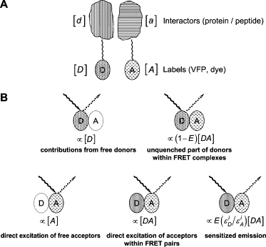
Conventions and fluorescence properties of interacting molecules. (A) We consider interactors d and a, which can be present either as separate molecules at abundances [d] and [a], respectively, or else as complexes at [da]. They are labeled with chromophores D (for donor) and A (for acceptor). Since labeling may not be complete and since fluorophores—even when present—may not be functional (either because of bleaching or incomplete folding), we distinguish between d and D (and a and A) and call [D] the abundance of those donor fluorophores, which are intact and coupled to a monomeric interactor of type d. Likewise, we call [A] and [DA] the abundances of intact fluorophores of monomeric type a and of complexes, da, respectively. Note that, in the latter case, both fluorophores have to be intact for da to qualify as DA. The relationship between [a], [d], and [da] on the one hand and [A], [D], and [DA] on the other, is given by Eqs. 28–30. We assume that the dimerization is not influenced by the labeling state of the interactors. (B) The upper row shows the fluorophore configurations leading to fluorescence with donor emission characteristics. These are the contributions to δⁱ of Eq. 14. The left side shows the emission from free donor D, which can be either a monomeric, correctly labeled molecule of type d (see above), or a dimer with an intact fluorophore D and a nonfluorescent (or nonexisting) label on a. The lower row shows the three contributions to fluorescence (Eq. 15) with emission spectrum of the acceptor.

Also, we describe some additional quantities, which are likely to be invariant during certain types of experiments. These are the total concentrations of labeled donor ([D^t]) and acceptor ([A^t]), as well as their ratio R^t. Furthermore, we describe a calibration procedure, based on measurements with cells expressing (or being labeled with) exclusively either donors or acceptors. In our equations, [D^t] and [A^t] are expressed in terms of the concentrations [D^ref] and [A^ref], which are present in the calibration samples. An additional measurement with a tandem construct allows us to determine the ratio [D^ref]/[A^ref], such that R^t can be specified as the actual molar ratio (except for ratios of folding or labeling probabilities).

In all cases, we assume that molecular interactions occur independently of the labeling state of the partners. Our method, which we call lux-FRET, is quite similar to sRET (32), except that we explicitly consider paired and unpaired chromophores, allow for incomplete labeling, and describe a simpler calibration procedure.

We apply the formalism to analyze fluorescence from cell suspensions measured in a calibrated spectrofluorometer. However, the approach is also readily applicable to imaging on a fluorescence microscope, both using traditional three-cube measurements and using spectrally resolved detectors and emission fingerprinting. The corresponding equations as well as calibration procedures are provided in Appendix 1.

Theory

Several recent studies have addressed the problem of extracting the apparent FRET-efficiency Ef_A from two-wavelength excitation measurements (15,21,23,24,33). Unfortunately, a multitude of different notations is used in these articles, such that comparison of results and an overview on the simplifying assumptions made, is difficult. Nevertheless, we will introduce another notation here for the following reasons:

• •Our approach derives equations on the basis of complete emission spectra, rather than signals from predefined spectral bands.
• •We avoid complicated expressions by introducing signals from discrete spectral bands only in the end (see Appendix 1), thus allowing our notation to be concise for most of the algebra.
• •Our notation is based on that used in spectroscopy (22), such that many elements actually are not new.

Calibration procedure and analysis of emission spectra

Four calibration spectra have to be obtained for a given pair of fluorophores and a given fluorimeter or microscope: Two emission spectra each at two excitation wavelength, using cells which either express exclusively donors or acceptors. We refer to these as $F_{\text{D}}^{\text{i,ref}}(\lambda )$ and $F_{\text{A}}^{\text{i,ref}}(\lambda ),$ respectively, where the superscript i (= 1,2) denotes the excitation wavelength and the subscripts D and A refer to donor and acceptor, respectively. The excitation wavelengths should be selected such that one of them (i = 1) excites mainly the donor fluorophore, while the other one (i = 2) excites mainly acceptor. In case the calibration samples have concentrations [D^ref] and [A^ref] for donor and acceptor fluorophores, respectively, the spectral intensities will be given by

$$F_{\text{D}}^{\text{i},\text{ref}}(\lambda )=I^{\text{i},\text{ref}}{\epsilon }_{\text{D}}^{\text{i}}{Q}_{\text{D}}{\eta }^{\text{i}}(\lambda )e_{\text{D}}(\lambda )[D^{\text{ref}}]\text{,}$$ (1)

$$F_{\text{A}}^{\text{i},\text{ref}}(\lambda )=I^{\text{i},\text{ref}}{\epsilon }_{\text{A}}^{\text{i}}{Q}_{\text{A}}{\eta }^{\text{i}}(\lambda )e_{\text{A}}(\lambda )[A^{\text{ref}}]\text{,}$$ (2)

where I^i,ref is excitation intensity and ${\epsilon }_{\text{D}}^{\text{i}},{\epsilon }_{\text{A}}^{\text{i}}$ are extinction coefficients of donor and acceptor at the two excitation wavelengths λⁱ (i = 1,2); Q_D, Q_A are quantum yields of donor and acceptor; and e_D(λ), e_A(λ) are standard emission spectra of the two fluorophores normalized to unit area. The functions ηⁱ(λ) are detection efficiencies of the instrument used and may be different for different excitation wavelengths due to differences in filters.

From the reference measurements (Eqs. 1 and 2) we can define the excitation ratios r^ex,i

$$r^{\text{ex},\text{i}}=\frac{F_{\text{D}}^{\text{i},\text{ref}}(\lambda )Q_{\text{A}}{e}_{\text{A}}(\lambda )}{F_{\text{A}}^{\text{i},\text{ref}}(\lambda )Q_{\text{D}}{e}_{\text{D}}(\lambda )}$$ (3)

for each of two excitation wavelengths (λⁱ). With Eqs. 1 and 2 these ratios are found to provide a link between absorption coefficients and dye concentrations:

$$\frac{{\epsilon }_{\text{D}}^{\text{i}}}{{\epsilon }_{\text{A}}^{\text{i}}}=r^{\text{ex},\text{i}}\frac{[{\text{A}}^{\text{ref}}]}{[{\text{D}}^{\text{ref}}]}\text{.}$$ (4)

Note that in these ratios the detection efficiencies have cancelled out, such that all measurements can also be performed on instruments without absolute calibration. The ratios of Eq. 3 can be calculated, provided the ratios of quantum efficiencies are known together with the corresponding emission spectra e_D(λ) and e_A(λ). In practice, we plot both the numerator of Eq. 3 and a scaled version of its denominator against λ, using values for the quantum efficiencies for cyan fluorescent protein (CFP) and yellow fluorescent protein (YFP) from the literature (Q_CFP = 0.4 (34) and Q_YFP = 0.61 (27)). The ratios r^ex,i are then found as the scaling factors of a least-square fit, which brings the two curves in register. Fig. 2 A, shows such a fit for excitation wavelength λ¹ = 458 nm, yielding r^ex,1 = 2.05. Fig. 2 B shows the same for excitation wavelength λ² = 488 nm, yielding r² = 0.02. The lower traces in this figure show the full ratios (Eq. 3) as a function of emission wavelength. It is seen, that these are reasonably constant, in the range where donor- and acceptor-emissions overlap.

Figure 2.

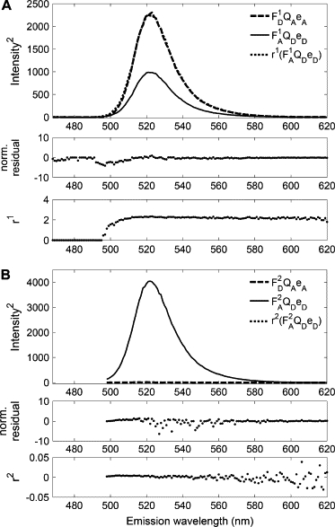
Calculation of excitation ratios r^ex,i: Fluorescence reference spectra of CFP (numerator of Eq. 3) are fitted to YFP reference spectra (denominator of Eq. 3), resulting in a scaling factor r^ex,1 = 2.29 for data obtained using excitation wavelength λ² = 458 nm (A). The same procedure applied to data with excitation wavelength λ² = 488 nm result in r^ex,2 = 0.02 (B). The two lower panels in both panels A and B show the residuals of the fits and the ratios r^ex,i as functions of emission wavelength.

In the case that the measurements are performed on an absolutely calibrated spectrofluorometer (such as the Fluorolog used in the measurements reported here), the ratios $F_{\text{D}}^{\text{ref}}(\lambda )/e_{\text{D}}(\lambda )$ and $F_{\text{A}}^{\text{ref}}(\lambda )/e_{\text{A}}(\lambda )$ are just the normalization constants of the two reference spectra $n_{\text{A,D}}^{\text{i}}\text{,}$ such that Eq. 3 simplifies to

$$r^{\text{ex},\text{i}}=\frac{n_{\text{D}}^{\text{i}}{Q}_{\text{A}}}{n_{\text{A}}^{\text{i}}{Q}_{\text{D}}}\text{.}$$ (5)

The four reference spectra $F_{\text{D}}^{\text{i},\text{ref}}$ and $F_{\text{A}}^{\text{i},\text{ref}}$ (not normalized) as well as the two ratios r^ex,i (i = 1,2) represent the result of the calibration procedure.

Basic equations and assumptions for FRET measurements

For the test measurement, we consider a sample, which contains both free donor at concentration [D], as well as free acceptor at [A] and the complex [DA], where the capital letters denote molecules with intact labels, as explained in Fig. 1. The influence of incomplete labeling will be considered in the next section. We will measure an emission spectrum (23,31,35), which is a linear combination of five contributions, two of which have the emission characteristics of the donor (the contributions from free donors and the unquenched part of fluorescence from donors within FRET complexes), the remaining three with the emission characteristics of the acceptor (i.e., direct excitation of free acceptors, of acceptors within FRET pairs, and sensitized emission) (Fig. 1):

$$\begin{array}{l}{F}^{\text{i}}(\lambda )=I^{\text{i}}{\eta }^{\text{i}}(\lambda )({\epsilon }_{\text{D}}^{\text{i}}{Q}_{\text{D}}{e}_{\text{D}}(\lambda )[D]+{\epsilon }_{\text{D}}^{\text{i}}{Q}_{\text{D}}{e}_{\text{D}}(\lambda )[\text{DA}](1-E)\\ +{\epsilon }_{\text{A}}^{\text{i}}{Q}_{\text{A}}{e}_{\text{A}}(\lambda )[A]+{\epsilon }_{\text{A}}^{\text{i}}{Q}_{\text{A}}{e}_{\text{A}}(\lambda )[\text{DA}]\\ +{\epsilon }_{\text{D}}^{\text{i}}{Q}_{\text{A}}{e}_{\text{A}}(\lambda )[\text{DA}]E).\end{array}$$ (6)

Sorting these terms according to those with emission characteristics of the donor and acceptor, respectively, we obtain

$$\begin{array}{l}{F}^{\text{i}}(\lambda )=I^{\text{i}}{\eta }^{\text{i}}(\lambda )\left({\epsilon }_{\text{D}}^{\text{i}}{Q}_{\text{D}}{e}_{\text{D}}(\lambda )([\text{D}]+(1-E)[\text{DA}])\right)\\ \left(+{\epsilon }_{\text{A}}^{\text{i}}{Q}_{\text{A}}{e}_{\text{A}}(\lambda )\left([\text{A}]+\left(1+E\frac{{\epsilon }_{\text{D}}^{\text{i}}}{{\epsilon }_{\text{A}}^{\text{i}}}\right)[\text{DA}]\right)\right)\end{array}$$ (7)

and eliminating spectral parameters by use of the reference spectra (Eqs. 1 and 2), we obtain:

$$\begin{array}{l}{F}^{\text{i}}(\lambda )=\frac{I^{\text{i}}}{I^{\text{i},\text{ref}}}\left(F_{\text{D}}^{\text{i},\text{ref}}(\lambda )\frac{([\text{D}]+(1-\text{E})[\text{DA}])}{[{\text{D}}^{\text{ref}}]}\right)\\ \left(+F_{\text{A}}^{\text{i},\text{ref}}(\lambda )\frac{([\text{A}]+(1+E{\epsilon }_{\text{D}}^{\text{i}}/{\epsilon }_{\text{A}}^{\text{i}})[\text{DA}])}{[{\text{A}}^{\text{ref}}]}\right).\end{array}$$ (8)

If we fit the measured spectrum F_i(λ) by a linear combination of $F_{\text{D}}^{\text{i},\text{ref}}$ and $F_{\text{A}}^{\text{i},\text{ref}}$:

$$F^{\text{i}}(\lambda )={\delta }^{\text{i}\ast }{F}_{\text{D}}^{\text{i},\text{ref}}+{\alpha }^{\text{i}\ast }{F}_{\text{A}}^{\text{i},\text{ref}}\text{.}$$ (9)

We note that

$${\delta }^{\text{i}\ast }=\frac{I^{\text{i}}}{I^{\text{i},\text{ref}}}\frac{([\text{D}]+(1-\text{E})[\text{DA}])}{[{\text{D}}^{\text{ref}}]}\text{,}$$ (10)

$${\alpha }^{\text{i}\ast }=\frac{I^{\text{i}}}{I^{\text{i},\text{ref}}}\frac{([\text{A}]+(1+E{\epsilon }_{\text{D}}^{\text{i}}/{\epsilon }_{\text{A}}^{\text{i}})[\text{DA}])}{[{\text{A}}^{\text{ref}}]}\text{.}$$ (11)

Introducing

$${\delta }^{\text{i}}=\frac{I^{\text{i},\text{ref}}}{I^{\text{i}}}{\delta }^{\text{i}\ast }\text{,}$$ (12)

$${\alpha }^{\text{i}}=\frac{I^{\text{i},\text{ref}}}{I^{\text{i}}}{\alpha }^{\text{i}\ast }\text{,}$$ (13)

we obtain, together with Eq. 8,

$${\delta }^{\text{i}}=\frac{[\text{D}]+(1-E)[\text{DA}]}{[{\text{D}}^{\text{ref}}]}$$ (14)

$${\alpha }^{\text{i}}=\frac{[\text{A}]+[\text{DA}]+({\epsilon }_{\text{D}}^{\text{i}}/{\epsilon }_{\text{A}}^{\text{i}})E[\text{DA}]}{[{\text{A}}^{\text{ref}}]}\text{.}$$ (15)

We call the quantities αⁱ and δⁱ, apparent relative acceptor and donor concentrations, respectively, since a mixture of free [D] and free [A] at these concentrations would yield the same emission characteristics. The individual terms of the numerators of Eqs. 14 and 15 are the contributions mentioned above (see also (23,31,35)).

If there are two measurements available at two excitation wavelengths λⁱ (i = 1,2), then Eqs. 14 and 15 represent three independent equations (Eq. 14 is identical for the two wavelengths, since it does not depend on the extinction ratio) and the three unknowns [D], [A], and [DA] are readily calculated from Eqs. 14 and 15.

Using the abbreviations

$$\Delta \alpha ={\alpha }^2-{\alpha }^1\text{,}$$ (16)

$$\Delta r=r^{\text{ex},2}-r^{\text{ex},1}\text{,}$$ (17)

we obtain

$$[\text{D}]=[{\text{D}}^{\text{ref}}]\left({\delta }^1-\frac{\Delta \alpha }{\Delta r}\frac{1-E}{E}\right)\text{,}$$ (18)

$$[\text{A}]=\frac{[{\text{A}}^{\text{ref}}]}{\Delta r}\left({\alpha }^2{r}^{\text{ex},1}-{\alpha }^1{r}^{\text{ex},2}-\frac{\Delta \alpha [{\text{D}}^{\text{ref}}]}{E[{\text{A}}^{\text{ref}}]}\right)\text{,}$$ (19)

$$[\text{DA}]=[{\text{D}}^{\text{ref}}]\frac{\Delta \alpha }{E\Delta r}\text{.}$$ (20)

Unfortunately, these equations are not of much use, unless E is known precisely. However, this is rarely the case in practice, particularly when one has to consider incomplete labeling. On the other hand, Eqs. 14 and 15 can be transformed into a set of linear equations (Eq. 23) with variables, which are convenient for formulating the effects of incomplete labeling (see below). These are the total concentrations of intact donor and acceptor fluorophores [D^t], and [A^t] and the product E[DA]. With Eqs. 18–20 we obtain

$$[{\text{D}}^{\text{t}}]\equiv [\text{D}]+[\text{DA}]=[{\text{D}}^{\text{ref}}]\left({\delta }^1+\frac{\Delta \alpha }{\Delta r}\right)\text{,}$$ (21)

$$[{\text{A}}^{\text{t}}]\equiv [\text{A}]+[\text{DA}]=[{\text{A}}^{\text{ref}}]\frac{({\alpha }^1{r}^{\text{ex},2}-{\alpha }^2{r}^{\text{ex},1})}{\Delta r}\text{,}$$ (22)

$$E[\text{DA}]=[{\text{D}}^{\text{ref}}]\frac{\Delta \alpha }{\Delta r}\text{,}$$ (23)

or else, expressed as apparent FRET-efficiencies,

$$E{f}_{\text{D}}\equiv E\frac{[\text{DA}]}{[{\text{D}}^{\text{t}}]}=\frac{\Delta \alpha }{\Delta r{\delta }^1+\Delta \alpha }\text{,}$$ (24)

$$E{f}_{\text{A}}\equiv E\frac{[\text{DA}]}{[{\text{A}}^{\text{t}}]}=\frac{[{\text{D}}^{\text{ref}}]}{[{\text{A}}^{\text{ref}}]}\frac{\Delta \alpha }{{\alpha }^1{r}^{\text{ex},2}-{\alpha }^2{r}^{\text{ex},1}}\text{,}$$ (25)

with the definitions

$$f_{\text{D}}\equiv [\text{DA}]/[{\text{D}}^{\text{t}}]\text{and}{f}_{\text{A}}\equiv [\text{DA}]/[{\text{A}}^{\text{t}}]\text{,}$$ (26)

which represent the fractions of D and A participating in FRET complexes.

For later use, we also define the ratio of acceptor and donor concentrations

$$R^{\text{t}}\equiv \frac{[{\text{A}}^{\text{t}}][{\text{D}}^{\text{ref}}]}{[{\text{D}}^{\text{t}}][{\text{A}}^{\text{ref}}]}=\frac{{\alpha }^1{r}^{\text{ex},2}-{\alpha }^2{r}^{\text{ex},1}}{\Delta r{\delta }^1+\Delta \alpha }\text{.}$$ (27)

Equation 24 allows the calculation of Ef_D from experimental quantities, without any additional information. Equations 25 and 27, on the other hand, depend on concentrations of donor and acceptor in the two samples, which were used for obtaining reference spectra. These are, so far, unknown, but their ratio can be obtained from a measurement on a tandem construct, as will be shown below.

Influence of incomplete labeling

So far, Eqs. 1–27 were written in terms of concentrations of those molecules, which are labeled with intact fluorophores. We designated these with capital letters ([D], [A], and [DA]). Now we will turn to the problem in which, in practice, we hardly ever encounter samples—the one where all molecules of interest carry intact labels. Possible reasons for incomplete labeling (incorrect folding, bleaching, wild-type molecules) were discussed in the Introduction. As stated before, we will designate chemical species of the molecules involved with lower-case letters (see Fig. 1), and use chemical concentrations [d], [a], and [da] for free molecular species d and a, as well as for da complexes, irrespective of their labeling state. We introduce labeling probabilities p_d and p_a and—for simplicity—do not distinguish whether the lack of a functioning label is due to incomplete labeling, folding, or bleaching. We also, following Clegg (31), assume that the labeling state does not influence the interaction.

With these assumptions we can write

$$[\text{D}]=p_{\text{d}}([\text{d}]+(1-p_{\text{a}})[\text{da}])$$ (28)

$$[\text{A}]=p_{\text{a}}([\text{a}]+(1-p_{\text{d}})[\text{da}])$$ (29)

$$[\text{DA}]=p_{\text{d}}{p}_{\text{a}}[\text{da}]$$ (30)

$$[{\text{D}}^{\text{t}}]=p_{\text{d}}[{\text{d}}^{\text{t}}]$$ (31)

$$[{\text{A}}^{\text{t}}]=p_{\text{a}}[{\text{a}}^{\text{t}}]\text{,}$$ (32)

where [d^t] and [a^t] represent total chemical concentrations of donors and acceptors, respectively.

The second terms in Eqs. 28 and 29 represent donor-acceptor complexes, in which either the acceptor molecule (Eq. 28) or the donor molecule (Eq. 29) is nonfluorescent.

The advantage of expressing results in terms of products of E and either f_D or f_A becomes evident when inserting Eqs. 28–30 into the definition for the latter two quantities (Eq. 26):

$$f_{\text{D}}=[\text{DA}]/([\text{D}]+[\text{DA}])=p_{\text{a}}{f}_{\text{d}}\text{,}$$ (33)

$$f_{\text{A}}=[\text{DA}]/([\text{A}]+[\text{DA}])=p_{\text{d}}{f}_{\text{a}}\text{.}$$ (34)

Here f_d and f_a are the fractions of d and a, respectively, participating in complexes in analogy to Eq. 26 except that we are considering chemical species irrespective of their labeling state.

With Eqs. 30–34 all the equations above can readily be written in a form, which include the influence of incomplete labeling. Before doing so, however, we will eliminate the ratio [D^ref]/[A^ref] by invoking a measurement on a tandem construct (which may be considered to be part of the calibration procedure).

Information obtained from a tandem construct

The missing piece of information for calculating Ef_A can be obtained by performing a measurement on a sample, which contains a tandem construct of one donor and one acceptor and no other fluorophores. Assuming that the tandem construct is chemically pure and that donor and acceptor moieties are correctly folded with probabilities p_d,tc and p_a,tc, respectively, we can set [d^t] = [a^t] and obtain from Eqs. 27, 31, and 32:

$$\frac{p_{\text{a},\text{tc}}}{p_{\text{d},\text{tc}}}=\frac{[{\text{D}}^{\text{ref}}]}{[{\text{A}}^{\text{ref}}]}={\left(\frac{{\alpha }^1{r}^{\text{ex},2}-{\alpha }^2{r}^{\text{ex},1}}{\Delta r{\delta }^1+\Delta \alpha }\right|}_{\text{Tandem}\text{Construct}}\equiv R_{\text{TC}}\text{.}$$ (35)

Here we introduce R_TC (TC: tandem construct) as a purely experimental parameter in analogy to R_t (Eq. 27), which is (up to a ratio of folding probabilities) equal to the ratio of fluorophore concentrations in the calibration samples.

Remarkably, Eq. 35 does not contain the FRET-efficiency of the tandem construct (E_TC), such that the ratio of concentrations in the reference samples (apart from the factor p_a,tc/p_d,tc) can be obtained without knowledge of E_TC. Below, we will use R_TC to eliminate the ratio [D^ref]/[A^ref] from some of the equations.

Hoppe et al. (15) also proposed equations for f_D and f_A and a concentration ratio R obtained from donor and acceptor fluorescence intensities. However, their method requires measurements using a donor-acceptor tandem construct with FRET efficiency previously obtained from fluorescence lifetime measurements.

Invariants and single wavelength measurements

In the above formalism, we defined several quantities, some of which may be invariant or may change only slowly during certain types of measurement. For instance, for any association reaction in a closed compartment or between two membrane-bound partners the total concentrations of donors and acceptors ([D^t], [A^t]; Eqs. 21 and 22) will be constant, when an average over the whole compartment or over a sufficiently large region of membrane or volume is taken, such that diffusion in and out of the compartment can be neglected. Likewise, the ratio R^t (Eq. 27) should be constant and bleaching will lead only to slow changes in these quantities. This opens up a number of possibilities for efficient and rapid tracking of dynamic changes in the interactions. For instance, one can determine R^t by a dual excitation measurement (Eq. 27), using a sample under stationary conditions. This measurement can be performed quite accurately, if a sufficiently long exposure time is used. Subsequently, one can perform single excitation measurements rapidly (see below), while stimulating a signaling reaction. Once the reaction comes to an end, R^t can be measured again with the full dual excitation procedure for a test, whether R^t has indeed been stationary. Likewise, total fluorophore concentrations [A^t] and [D^t] can be monitored according to Eqs. 21 and 22 to test for bleaching effects.

To obtain an equation, which contains R^t instead of one of the estimates for α, we calculate αⁱ/δ¹, using Eqs. 4, 14, and 15, and solve for

$$E{f}_{\text{D}}\equiv \frac{E[\text{DA}]}{[{\text{D}}^{\text{t}}]}=1-\frac{r^{\text{ex},\text{i}}+R^{\text{t}}}{r^{\text{ex},\text{i}}+{\alpha }^{\text{i}}/{\delta }^1}=\frac{{\alpha }^{\text{i}}/{\delta }^1-R^{\text{t}}}{r^{\text{ex},\text{i}}+{\alpha }^{\text{i}}/{\delta }^1}\text{.}$$ (36)

This equation is valid for either of the two excitation wavelengths λⁱ. It has valuable properties in both cases: For i = 1 (excitation at the donor wavelength) it contains only the ratio α¹/δ¹ except for the invariants R^t and r^ex,1. This means Ef_D can be evaluated from a single excitation only, which may be desirable for studying dynamic processes. For i = 2 it contains only the ratio α²/δ¹. This may be advantageous for optimizing signal resolution, since excitation intensities can be adjusted, such that both signals are of similar strength and resolution. Equation 36 is particularly suitable for analyzing fluorescence from tandem constructs, when R^t should be constant (except for bleaching) and, like r^ex,1, which needs to be evaluated only once for a given set of calibration spectra.

In this context, it should be pointed out that Eq. 25 also represents a special case in the sense that it depends only on invariants and the relative apparent acceptor concentrations αⁱ. If an instrument is available, which allows for rapid changes in excitation wavelength, measurement of emission can be restricted to a single spectral window, which passes only acceptor fluorescence. This may be an advantage, when only a single detector for emission is available.

Summary of equations

Here we summarize the equations derived above. We write them in a form that apparent quantities, which contain experimental parameters only, appear on the right side. On the left side we write a product of the quantities of interest (such as E[da], Ef_d, etc.) and a correction or scaling factor. The equations are either replicas of Eqs. 21–25 or derived from them, using, in addition, Eqs. 27 and 35 as well as Eqs. 28–34 for conversion of fluorophore concentrations into chemical concentrations. Equation 39 is provided in a form containing R^t, which is particularly suitable when the latter is invariant, as pointed out in the last section (see Appendix 2 for definition of symbols).

Apparent abundance of the FRET-complex:

$$E[\text{da}]\frac{p_{\text{d}}{p}_{\text{a}}}{[{\text{D}}^{\text{ref}}]}=\Delta \alpha /\Delta r\text{.}$$ (37)

Apparent FRET-efficiency (related to total donor):

$$E{f}_{\text{d}}{p}_{\text{a}}=\frac{\Delta \alpha }{\Delta r{\delta }^1+\Delta \alpha }$$ (38)

$$=\frac{{\alpha }^{\text{i}}/{\delta }^1-R^{\text{t}}}{{\alpha }^{\text{i}}/{\delta }^1+r^{\text{ex},\text{i}}}(\text{valid}\text{for}\text{both}i=1\text{and}i=2)\text{.}$$ (39)

Apparent FRET-efficiency (related to total acceptor):

$$E{f}_{\text{a}}{p^{\prime }}_{\text{d}}=R_{\text{TC}}\frac{\Delta \alpha }{{\alpha }^1{r}^{\text{ex},2}-{\alpha }^2{r}^{\text{ex},1}}\text{,}$$ (40)

$$=\frac{R_{\text{TC}}}{r^{\text{ex},1}}\left(\frac{{\alpha }^1}{{\alpha }^2}-1\right)\text{for}({\alpha }^1{r}^{\text{ex},2}\ll {\alpha }^2{r}^{\text{ex},1})\text{.}$$ (41)

Apparent ratio of fluorophores:

$$\frac{[{\text{a}}^{\text{t}}]}{[{\text{d}}^{\text{t}}]}\frac{p_{\text{a}}}{{p^{\prime }}_{\text{d}}}=R^{\text{t}}/R_{\text{TC}}\text{.}$$ (42)

Apparent total donor concentration:

$$[{\text{d}}^{\text{t}}]\cdot \frac{p_{\text{d}}}{[{\text{D}}^{\text{ref}}]}=(\Delta r{\delta }^1+\Delta \alpha )/\Delta r\text{.}$$ (43)

Apparent total acceptor concentration:

$$[{\text{a}}^{\text{t}}]\cdot \frac{p_{\text{a}}}{[{\text{A}}^{\text{ref}}]}=({\alpha }^1{r}^{\text{ex},2}-{\alpha }^2{r}^{\text{ex},1})/\Delta r\text{.}$$ (44)

Here, the abbreviation

$${p^{\prime }}_{\text{d}}=\frac{p_{\text{d}}{p}_{\text{a},\text{tc}}}{p_{\text{d},\text{tc}}}$$ (45)

was used.

When applying these equations to chemically pure tandem constructs, f_d and f_a are 1 by definition. In that case, a decision has to be made whether R_TC should be considered a calibration parameter (as determined once for a given calibration) or else be measured individually on a given sample. In the first case, Eqs. 38 and 40 are identical by definition. In the second case, we obtain by evaluating the right side of Eq. 38 the quantity Ep_a, which changes, when the acceptor is bleached or its folding state changes. We will show an example of this use in Results, analyzing a series of measurements, in which the donor is gradually bleached. In general, bleaching the fluorophores will enter into the equations as changes in p_a and p_d, such that an observed change in the experimental estimates (right sides of Eqs. 37–42) cannot be unambiguously associated with either bleaching or a change in E. However, if one can assume [a^t] and [d^t] to be constant, then a change in E should leave the results of Eqs. 43 and 44 unchanged. In the Appendix, we will present a set of equations in which this assumption is used to dissociate between changes in E and those in bleaching. It should be cautioned, though, that all of our equations are valid only if bleaching is small within a pair of excitations. In Appendix 1, we show that acceptor photobleaching, analyzed the usual way, also returns the product Ef_dp_a.

In summary, we conclude that for a precise measurement of the FRET-efficiency, E, we need a perfectly labeled acceptor species (i.e., p_a = 1) in the absence of any free donor (f_d = 1, i.e., acceptor excess). In this case, E should be evaluated according to Eq. 38 or 39. Alternatively, Eq. 40 allows one to evaluate E with a perfectly labeled donor species, which is in excess of the acceptor. In this case, an additional requirement is p_a,tc/p_d,tc = 1. These two approaches correspond to donor quenching and sensitized emission, respectively.

Materials and methods

Recombinant DNA procedures

All basic DNA procedures were performed as described by Sambrook et al. (36). To prepare YFP-CFP tandem constructs, cDNA encoding the enhanced YFP (Clontech, Palo Alto, CA) was amplified with primer YFP-EcoRI-sense primer (5′-C GAA TTC ATG GTG AGC AAG GGC GAG GAG CTG-3′) and YFP-BamHI-EK-antisense primer (5′-G TGG ATC CCG CTT ATC GTC ATC GTC CTT GTA CAG CTC GTC-3′), where EK is an abbreviation for enterokinase. The amplified fragments were cloned into the EcoR1 and BamHI restriction sites of the pECFP-N1 vector (Clontech), so that the YFP coding sequence was located in-frame of the N-terminal end of the CFP. By using this strategy, a fusion protein containing a 12-amino-acid linker between YFP and CFP was created. In addition, this linker also contains a recognition amino-acid sequence -Asp-Asp-Asp-Asp-Lys- for the enterokinase. The construct was verified by dideoxy DNA sequencing of the final plasmids.

Adherent cell culture and transfection

Mouse neuroblastoma N1E-115 cells were grown in Dulbecco's modified Eagle's medium containing 10% fetal calf serum and 1% penicillin/streptomycin at 37°C under 5% CO₂. For transient transfection, cells were seeded at low-density (1 × 10⁶) in 60-mm dishes and transfected with appropriate vectors using Lipofectamine2000 Reagent (Invitrogen, Carlsbad, CA) according to the manufacturer's instruction. Transfected cells were serum-starved for ∼20 h before analysis.

For experiments on a spectrofluorometer, 4 × 10⁶ cells were suspended in 2 ml of phosphate-buffered saline (PBS) with osmolarity adjusted with glucose to that of the culture medium (∼351 Osm/kg). Cell suspensions were filled into quartz cuvettes and maintained at 37°C in the acquisition chamber of the spectrofluorometer under stirring.

Fluorescence measurements

Fluorescence spectra were monitored at 37°C on a Fluorolog-3 spectrofluorometer (Horiba Jobin Yvon, München, Germany) with 2-nm spectral resolution for excitation and emission. Samples were placed in 10-mm pathway quartz cuvettes (10 × 10 mm²) and continuously stirred by a magnetic stirrer. The spectral contributions due to light scattering and nonspecific fluorescence of the cells were taken into account by including the emission spectra of nontransfected cells (background) as additional components during the fitting of the fluorescence spectra of cells expressing fluorescent protein constructs.

Single cell acceptor photobleaching and apparent FRET measurement

N1E-115 cells were transfected with a plasmid encoding for CFP-YFP tandem construct. Twenty-four hours after transfection cells were fixed by incubation in 4% paraformaldehyde/PBS for 10 min. Free aldehyde groups were quenched with 50 mM glycine for 15 min. Coverslips were washed in PBS and water and mounted on glass slides in 90% glycerine/H₂O solution. Images of cells expressing a cytosolic CFP-YFP fusion protein were acquired using a Zeiss LSM 510 Meta confocal microscope (Carl-Zeiss, Jena, Germany) with a 40×/1.3 NA oil-immersion objective using the 458 nm line of a 40 mW argon laser at 50% power and 5% transmission at a pixel resolution of 512 × 512. Lambda stacks of a 2-μm optical slice were acquired from 475 to 625 nm in 10.7 nm steps. A time series of eight frames was acquired over 124 s. Bleaching of acceptor (YFP) in a selected 20 pixel × 20 pixel region of interest was performed after the first four image acquisitions with the 514-nm line of the Argon laser at 50% power and 100% transmission for 300 iterations using a 458 nm/514 nm dual dichroic mirror. Linear unmixing was performed by the Zeiss AIM software package using CFP and YFP reference spectra obtained from cells expressing only cytosolic CFP or YFP. The same laser and microscope settings were used for test and calibration measurements. Apparent FRET efficiency was calculated offline as [(1-(CFP prebleach/CFP postbleach))] using fluorescence values that had been background-subtracted and corrected for acquisition bleaching, as determined from an unbleached region of interest.

Fluorescence lifetime measurement

Fluorescence intensity decays were obtained by time-correlated single photon-counting measurements of fluorescence using a Fluorolog-3 spectrofluorometer (Horiba Jobin Yvon). Samples were placed in 10-mm pathway quartz cuvettes (10 × 10 mm²) and continuously stirred with a magnetic stirrer. Emission was collected in right-angle geometry. Excitation was performed with a 460 nm nanoLED with a 440/40 nm transmission filter (Semrock, Tubingen, Germany). Fluorescence intensity was collected in the wavelength band from 468 nm to 482 nm to avoid acceptor fluorescence.

Typical fluorescence decays were fitted with the resulting sum of one, two, or three exponentials, interactively convolved with the instrument response function using the standard DataStation analysis software provided by Horiba Jobin Yvon and CFS_LS software (available from Center for Fluorescence Spectroscopy at http://cfs.umbi.umd.edu/cfs/software/). The quality of the fits was evaluated by the structure observed in the plots of residuals and by the reduced χ-square values. The mean fluorescence lifetimes were calculated as the mean values of the fit functions.

Results

Calibration measurements

The calibration was performed with the use of cells expressing exclusively either donor or acceptor at unknown concentration [D^ref] and [A^ref], respectively, using a calibrated spectrofluorometer (see Materials and Methods). To obtain the emission characteristics of donor, e_D(λ), and acceptor, e_A(λ) fluorophores, complete fluorescence emission spectra were collected from suspensions of N1E-115 neuroblastoma cells expressing either cytosolic CFP (donor) or YFP (acceptor). These acquisitions were performed with excitation at 420 and 458 nm, respectively, with fluorescence emission collected from 430 to 620 and 468 to 620 nm (see Materials and Methods). The spectra were normalized to unit area, resulting in e_D(λ) and e_A(λ) as shown in Fig. 3. Similarly, spectra were collected from both cell types at two specific excitation wavelengths λ¹ = 458 nm and λ² = 488 nm. These spectra were not normalized and we denote them as reference spectra $F_{\text{D}}^{1,\text{ref}}(\lambda ),F_{\text{D}}^{2,\text{ref}}(\lambda ),F_{\text{A}}^{1,\text{ref}}(\lambda )\text{,}$ and $F_{\text{A}}^{2,\text{ref}}(\lambda )\text{,}$ according to the notation introduced above. Subscripts D and A refer to Donor (CFP) and Acceptor (YFP), and superscripts 1 and 2 to the two excitation wavelengths, respectively. Note that these spectra are not identical to e_D(λ) and e_A(λ) above, because they are measured at different excitation wavelengths and may be curtailed at short wavelengths.

Figure 3.

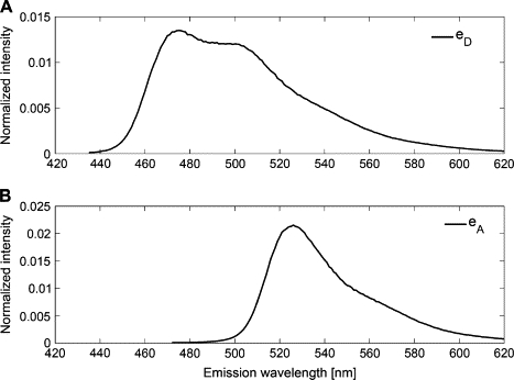
Reference spectra. Fluorescence emission reference spectra of CFP (A) at excitation wavelength λ_exc = 420 nm and YFP (B) at λ_exc = 458 nm are normalized to unit area.

The calibration also requires excitation ratios, r^ex,i, according to Eq. 3. These values were determined from the above spectra as r^ex,1 = 2.05, r^ex,2 = 0.02, using quantum yield values of donor and acceptor, Q_D = 0.4 and QA = 0.61, respectively, from the literature (34,27) as detailed in a previous section. On average, the values were r^ex,1 = 2.26 ± 0.26 (mean ± SD, n = 4) and r^ex,2 = 0.01 ± 0.01.

FRET efficiency of the tandem construct

We performed a first set of test measurements with cells expressing a cytosolic tandem construct (TC) of donor and acceptor fluorophores. Emission spectra were collected using the same excitation wavelengths λ¹ = 458 nm and λ² = 488 nm, and the same intensities as used during the calibration measurements. We determined the apparent acceptor αⁱ and donor δⁱ concentrations by least-square fitting of a superposition of the two reference spectra to the spectra of TC-expressing cells. A small third component, proportional to the background fluorescence of nontransfected cells, was included in the fit to compensate for residual autofluorescence and light scattering. The estimated parameters (weights of these fits) were α¹ = 1.63, α² = 0.78, and δ¹ = 0.65. The procedure for obtaining these quantities with the relevant spectra is exemplified in Fig. 4 (see Fig. 4 legend for further details).

Figure 4.

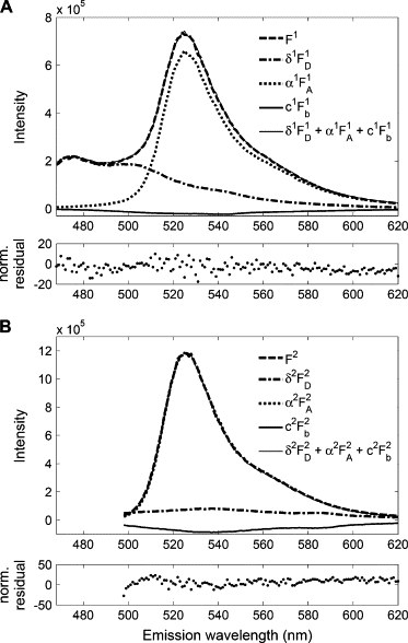
Spectral analysis of fluorescence from a cytosolic CFP-YFP tandem construct using excitation at λ¹ = 458 nm (A) and λ² = 488 nm (B). The upper panels show superpositions of the measured spectra (Fⁱ) with reference spectra of donor $(F_{\text{D}}^{\text{i}}),$ acceptor $(F_{\text{A}}^{\text{i}}),$ and background spectra $(F_{\text{b}}^{\text{i}})\text{.}$ The latter spectra were scaled such that they add up to fit the measured spectra. The scaling factors αⁱ and δⁱ are the sought-for apparent relative concentrations. Lowermost traces in both panels A and B show the residuals of the fits.

The values for r^ex,i, αⁱ, and δⁱ were used with Eqs. 38 and 40 to calculate the apparent FRET efficiencies E_TC = 0.37 and [A^ref]/[D^ref]E_TC = 0.48. Applying Eq. 35, we can calculate the quantity R_TC, which is the ratio of fluorophore concentrations [D^ref]/[A^ref] in the reference samples during calibration (apart from labeling probabilities). It was found to be R_TC = 0.76. Thus (by necessity), the value for E_TC according to Eq. 40 is also 0.37. In eight experiments of this type, the mean value (± SD) was R_TC = 0.68 ± 0.05 and E_TC = 0.389 ± 0.027.

These values are in line with the FRET efficiency obtained from acceptor photobleaching experiments on a laser scan microscope using fixed N1E-115 cells expressing the CFP-YFP tandem construct (see Fig. 5 for details) and with cuvette experiments on partial photobleaching (see next section).

Figure 5.

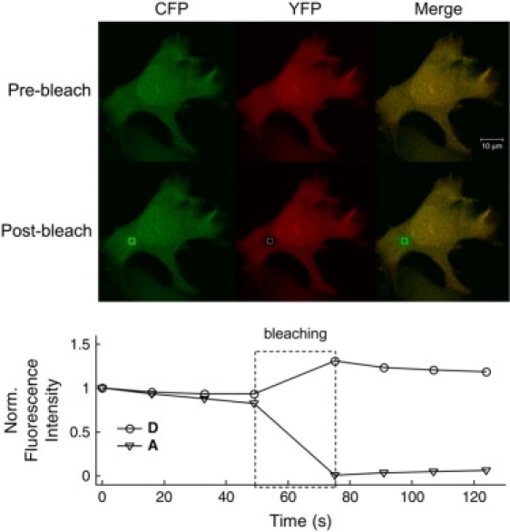
Acceptor photobleaching experiment on N1E-115 cells expressing a cytosolic CFP-YFP tandem construct. White boxes correspond to the bleached regions of interest. (Upper panel) The fluorescence image of the CFP channel (green), the YFP channel (red), and composite channel before bleaching. (Lower panel) The same after bleaching. Below, the normalized 12-bit grayscale intensities of both channels YFP-acceptor (A) and of the CFP-donor (D) are plotted for the region-of-interest during the whole trial (scale bar represents 10 μm).

Considering that some donor or acceptor fluorophores may not be correctly folded, we realize that all the above numbers for E_TC actually are products of the true FRET-efficiency E and the probability that a given tandem construct carries an intact acceptor or donor (Eq. 38).

We also compared our value for FRET-efficiency of the tandem construct with that obtained from fluorescence lifetime measurements. To do so, we determined lifetime histograms for both cytosolic CFP as well as for CFP within the (CFP-YFP) tandem construct by time-correlated single photon counting as described in Material and Methods. In both cases the decay curves were analyzed by two-exponential fits and mean values of fluorescence lifetime were calculated. Since the mean fluorescence lifetime value shows slight variations between samples, values for different samples were averaged. The averaged fluorescence lifetime value for cytosolic CFP was found to be 〈τ〉_D = 2.44 ± 0.10 ns (n = 9). As we expected, the decay kinetics of CFP in the tandem construct were strongly affected by the presence of covalently linked acceptor (YFP moiety) and yielded a shortened average lifetime 〈τ〉_TC = 1.46 ± 0.14 ns (n = 6). From these average lifetimes (i.e., 〈τ〉_TC and 〈τ〉_D), the FRET-efficiency was calculated using the equation E_TC = 1−〈τ〉_TC/〈τ〉_D and found to be E_TC = 0.40 ± 0.06.

Partial photobleaching of the acceptor

Using the same experimental settings (i.e., same excitations wavelengths and intensities) as described before, we examined the effect of progressive acceptor photobleaching on apparent FRET efficiency of the cytosolic tandem construct. To do this, emission spectra were collected on the spectrofluorometer from N1E-115 cells expressing the cytosolic tandem construct using two excitation wavelengths λ¹ = 458 nm and λ² = 488 nm. Then cells were exposed to high excitation intensity at an excitation wavelength of 514 nm for several 2 h periods. In between exposures emission spectra were collected. To analyze these spectra the same reference spectra were used as obtained previously (see Calibration Measurements). The ratio of acceptor over donor concentrations, R^t (Eq. 27) changed from an initial value, which was set to 1, to a final value of 0.49 due to progressive bleaching of the acceptor.

According to Eqs. 38 and 40 (setting f_d = 1 and f_a = 1)), the product of the characteristic FRET efficiency and the labeling probabilities can be calculated. Before acceptor bleaching the values for donor and acceptor were equal ($E{p}_{\text{a}}=E{p^{\prime }}_{\text{d}}=0.425$, which is a consequence of setting R^t = 1). During acceptor bleaching the quantity Ep_a decreased, as expected, to a final value of 0.207, while $E{p^{\prime }}_d$ stayed approximately constant. Fig. 6 shows a plot of these values against [A^t]/[D^t]. As expected, a linear fit through the data points extrapolates to the origin, indicating that the estimate for total remaining acceptor fluorophore abundance is consistent with the estimate of labeling probability.

Figure 6.

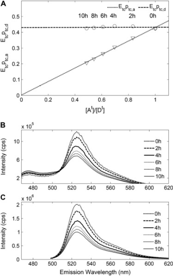
Partial acceptor photobleaching of a cytosolic tandem construct expressed in neuroblastoma N1E-115 cells. (A) The upper panel shows Ep_a and Ep_d values measured in 2 h intervals over a total of 10 h of acceptor photobleaching of a tandem construct expressed by N1E cells in a cuvette. Acceptor photobleaching decreases the measured Ep_a and [A^t]/[D^t], while Ep_d remains unchanged. The linear fits to the data suggest that with continued acceptor-photobleaching both Ep_a and [A^t]/[D^t] would reach 0, while Ep_d continues to be unaffected. (B) Emission spectra from the tandem construct excited at 458 nm during the bleaching experiment. Corresponding to the decrease in the peak at 525 nm, an increase in the peak at 475 nm is observed, resulting from the dequenching of CFP. (C) Emission spectra of the tandem construct excited at 488 nm show fluorescence intensity resulting mainly from direct excitation of YFP. Shown is a decrease of ∼50% over the course of photobleaching, resulting in the reduction of the calculated [A^t]/[D^t] from 1 to 0.5, as shown in panel A.

It was recently shown that photobleaching of YFP induces a weakly fluorescent fluorophore with CFP-like properties (37). Although fluorescence from that species is expected to be very low, when excited at 458 nm (37), we performed a control, in which we bleach a YFP sample using a very similar protocol. Spectral decomposition yielded a CFP-like contribution changing from 0.031 ± 0.009 to 0.032 ± 0.006 (in units of [D^ref]). Corresponding values obtained from the tandem construct acceptor photobleaching experiment shown on Fig. 6 are between 2.16 ± 0.02 and 2.98 ± 0.01. This demonstrates that the results of Fig. 6 are not compromised by the generation of a CFP-like fluorophore.

Discussion

For studying molecular interactions in a live cell environment, it would be most convenient to monitor the abundances or concentrations of the interacting partners [a], [d], and [da] in a temporally and spatially resolved manner. (Please note that we use lower-case letters for chemical species of interactors, irrespective of their labeling state; see Fig. 1 and Introduction.) Recording spectrally resolved images at two different excitation wavelengths in principle allows one to calculate abundances of intact fluorophores [A], [D], and [DA], either with conventional three-cube methods or by spectral fingerprinting, if the FRET-efficiency E of the donor-acceptor complex is known (23). We show here that, in practice, E cannot be determined accurately, unless one has a sample with only DA complexes (no free donors and free acceptors) and that all complexes are perfectly labeled (i.e., they carry intact fluorophores). If this is not the case, one can calculate from the spectral data products of the type Ef_A and Ef_D, where f_A,D represent the fractions of acceptor or donor fluorophores participating in FRET-complexes. We also show that the measurable quantities Ef_A and Ef_D are products of the type $E{f}_{\text{a}}{p^{\prime }}_{\text{d}}$ and Ef_dp_a, with p_d,a denoting the probabilities that a given donor/acceptor-molecule is actually fluorescent. The chemical fractions f_a, f_d depend on the stoichiometry of the ${p^{\prime }}_{\text{d}}$ interaction, on concentrations of the partners, as well as on their affinity, while the quantities ${p^{\prime }}_{\text{d}}$ and p_a reflect labeling efficiencies, probabilities of correct folding, bleaching, etc. The prime in ${p^{\prime }}_{\text{d}}$ reminds us of the fact that this quantity also depends on the folding state of the tandem construct, which is part of the calibration procedure.

We describe analysis procedures, in which—depending on the equations used—one obtains either $E{f}_{\text{a}}{p^{\prime }}_{\text{d}}$ or else Ef_dp_a as well as the total concentrations of intact fluorophores of type D and A, relative to the concentrations of calibration samples. Quantities like f_a and f_d are probably those parameters, which are most interesting for a biologist, who wants to study interactions among a and d. Unfortunately, spectral analysis of FRET provides them only as products together with E and folding/labeling probabilities, which are usually not known. Likewise, when studying intramolecular FRET (where f_a and f_d are equal to 1 by definition), one does not obtain E (which is a measure of distance and orientation between the two fluorophores) but instead a product, including folding/labeling probabilities. In the case of visible fluorescent proteins probabilities of correct folding have been reported to depend on cellular environment, temperature, and state of maturation of cells in culture (38) and to vary between 49 and 90% (39,40).

Excitation at two different wavelengths is required to calculate the quantities mentioned so far. However, our analysis points out certain conditions, in which excitation at a single wavelength suffice to obtain valuable information, as discussed in Invariants and Single Wavelength Measurements. This holds, whenever total concentrations of interactors (a,d) can be considered constant over time. Our equations allow the measurement of these or else of the ratio of total donors over acceptors. Once those are known, one can monitor temporal changes in the concentration of FRET-complexes [DA]. In the case of slowly varying parameters, such as when moderate bleaching occurs during a time series, one can measure total donor-acceptor fluorophore concentrations before and after the time series. The time course of [DA] can then be derived on the basis of an interpolation regarding the total concentrations. We demonstrate the correctness of our approach by measuring the FRET-efficiency of a tandem construct while partially bleaching the acceptor fluorophore. As expected, FRET-efficiency stays constant when measured by a procedure, which calculates Ep_d, while it decreases, when estimated via the analysis method, which returns Ep_a. Likewise E stayed constant, when evaluated by an equation, which is based on the measurement of the ratio of intact donors relative to acceptors. This demonstrates that this analysis method provides suitable corrections for slow bleaching effects, when monitoring intramolecular FRET of a FRET-based sensor.

Calibration procedures

The calibration of a FRET setup is usually performed by a set of measurements using samples of pure donor or acceptor, respectively, and suitable combinations of excitation wavelengths and spectral emission windows. These are selected to provide fluorescence readings, which represent predominantly either donor or acceptor fluorescence (24,13). Effects of bleedthrough (between spectral emission bands) and cross-talk (excitation of the wrong fluorophore) are taken care of by corrections to these readings (15,11). Our analysis method is based on full emission reference spectra and on fits of linear combinations of these to the emission spectra from test samples (or else from individual pixels in the case of images). This automatically includes the corrections for bleedthrough. Cross talk is explicitly included in our equations.

In practice it may be required to bin a few emission channels for reduction of the computational load. In this case the fitting can still be performed with correspondingly binned reference spectra. In the extreme case that the emission spectra are binned into two channels (one representing mainly donor fluorescence, the other mainly acceptor fluorescence) the fitting task is reduced to solving two sets of two linear equations (one for each excitation wavelength) for the unknowns δ¹, δ², α¹, and α². This procedure, which is analogous to the traditional three-cube technique, is described in the last section of the Appendix.

In addition to problems of cross talk and bleedthrough, any stoichiometric analysis of FRET signals is confronted with the problem that the ratio of molar extinction coefficients enters into the equations (e.g., Eq. 15). In some studies, this problem is solved by taking these ratios (one for each excitation wavelength) from the literature. However, such data may not be available. We offer a partial solution by defining the excitation ratios r^ex,i in our calibration procedure (Eq. 3). To calculate these we need from the literature only quantum efficiencies Q_A and Q_D, which are often easier to come by. We did not need any further literature data, since we measured our reference spectra on a calibrated spectrofluorometer. In the more general case, when spectra are measured with a noncalibrated detector, the ratio of normalized emission spectra, e_A(λ) over e_D(λ), is needed in addition (see Eq. 3). Unfortunately, a calibration without resorting to any literature data would require the measurement of molar extinction coefficients or else the measurement of relative extinction coefficients combined with a dual excitation experiment on a tandem construct (in analogy to the procedure leading to Eq. 35).

Correspondence to other analysis methods

A number of recent articles have addressed the problem of the stoichiometry of the interaction partners (15,24,32,33,41). As in the case of the study by Thaler and co-workers (32), we base the analysis on information from the full emission spectra. In addition, our expressions explicitly include contributions from simultaneously present donors, acceptors, and FRET-pairs. We describe a calibration procedure, which is less dependent on parameters from the literature (see discussion above), and we incorporate the effects of incompletely labeled interaction partners.

Some of our parameters correspond closely to parameters used by others. For instance, the ratio of total fluorophore abundances, [A^t]/[D^t], which can be calculated from Eqs. 22 and 21 converting donor and acceptor fluorescence intensities into total donor and acceptor concentration ratios, is similar to the formulas of Chen and co-workers (21) and Hoppe and co-workers (15). We should point out, however, that the method presented here allows us to calculate these quantities using a tandem construct even if it has no FRET or if it has an unknown FRET efficiency. Then, Chen et al. (21) use the so-called k-factor as the ratio of donor-to-acceptor fluorescence intensities for equimolar concentrations in the absence of FRET, while we determine the quantity R_TC, the apparent ratio of donors to acceptors of a tandem constructs, which is the inverse of that ratio in the reference samples. Zheng and Zagotta (42) define the FRET-ratio FR in their Eq. 10. The relationship to our approach is seen, when we consider Eq. 38 (r^ex,2 is 0.02 for excitation at 488 nm). We readily realize that FR is equivalent to α¹/α².

Another analogy can be demonstrated for a fluorophore- and instrument-specific quantity, the G-factor, defined as the ratio of sensitized emission to the quenched donor emission due to FRET (43). According to Eq. 7 this ratio is given by Q_Ae_A/Q_De_D, which with Eq. 3 is $(F_{\text{A}}^{\text{i},\text{ref}}/F_{\text{D}}^{\text{i},\text{ref}})r^{\text{ex},\text{i}}\text{.}$ Since our equations are expressed in terms of relative abundances (relative to $F_{\text{A}}^{\text{i},\text{ref}}$ and $F_{\text{D}}^{\text{i},\text{ref}}$), the parameter r^ex,1 will appear in our equations wherever the G-factor appears in the equations of Zal and Gascoigne (43). In this sense r^ex,1 is also equivalent to the factor γ/ξ, as defined and empirically determined by Hoppe and co-workers (15). Chen and co-workers (21) calculate the G-factor on the basis of two tandem constructs, while an equivalent quantity, the α-factor (44), is found by three tandem construct measurements.

The determination of apparent FRET efficiency in our method does not require, as in some other methods, acceptor photobleaching experiments (43) nor fluorescence lifetime measurements (15) or cell fixation (43).

Application to fluorescence microscopy

The measurements described here were performed on a spectrofluorometer by fitting spectra from test samples as linear superpositions of reference spectra, obtained on the same instrument. The output quantities of the fitting procedure (the relative apparent donor and acceptor concentrations δⁱ and αⁱ), however, are exactly the same numbers as returned for each pixel by a linear unmixing algorithm. Such algorithms (also called “spectral fingerprinting” or “emission fingerprinting”) are part of the analysis software of laser scan microscopes with spectrally resolved detection systems. It should thus be straightforward to apply all the equations of this work to individual pixels of a fluorescence image. Some practical considerations for such an application are given above in the discussion on calibration procedures and in the last section of the Appendix.

Appendix 1.

Separation of bleaching and changes in E

Whenever the total chemical concentrations of donors and/or acceptors are invariant during a series of measurements, Eqs. 3–44 can be used to calculate dynamic changes in E and p_a or p_d (bleaching) separately. For instance, Eqs. 43 and 44 can be considered as equations for p_d and p_a, each multiplied by an unknown, but constant factor (such as [d^t]/[D^ref] for Eq. 43 and [a^t]/[A^ref] for Eq. 44). Thus, we can readily follow dynamic changes in p_d and p_a by evaluating the terms on the right sides of these equations.

Inserting p_a and p_d, as obtained from Eqs. 43 and 44 into Eq. 37, we arrive at

$$E[\text{da}]=\frac{[{\text{d}}^{\text{t}}][{\text{a}}^{\text{t}}]}{[{\text{A}}^{\text{ref}}]}\frac{\Delta \alpha \Delta r}{({\alpha }^1{r}^{\text{ex},2}-{\alpha }^2{r}^{\text{ex},1})(\Delta r{\delta }^1+\Delta \alpha )}\text{.}$$ (46)

Dynamic changes in Ef_d and Ef_a are identical to those in E[da], since f_d and f_a are ratios of [da] with either [d^t] or [a^t], respectively, which we consider as constant for the moment.

Predictions for the association between donors and acceptors

In case the interaction partners d and a undergo a well-defined association reaction with dissociation constant K, we can apply the law of mass action to their chemical concentrations,

$$[\text{da}]=K^{-1}[\text{d}][\text{a}]\text{,}$$ (47)

or, in terms of the fractions of interacting species d and a in complexes,

$$K[\text{da}]=\frac{f_{\text{a}}}{1-f_{\text{a}}}\frac{f_{\text{d}}}{1-f_{\text{d}}}\text{.}$$ (48)

In principle, it is possible to express f_a and f_d in terms of Ef_A and Ef_D, which are measurable quantities, and the unknown parameters K[da] as well as products of E and the labeling probabilities p_d and p_a (see below). It may be possible to extract some of these parameters by a global analysis of images as has been performed by Erickson and co-workers (24). However, a straightforward analysis is only possible in limiting cases. For instance, if the reaction is of high affinity, such that [a^t] > K⁻¹ and [d^t] > K⁻¹, there is either no free a or free d, depending on which of the two reaction partners is in excess.

If, for instance, the donor is in excess, such that f_a = 1, we obtain from Eq. 40

$$E{p^{\prime }}_{\text{d}}=R_{\text{TC}}\frac{\Delta \alpha }{{\alpha }^1{r}^{\text{ex},2}-{\alpha }^2{r}^{\text{ex},1}}\text{,}$$ (49)

where all the quantities on the right-hand side of Eq. 49 are measurable.

Likewise, we obtain for the case of acceptor excess (f_d = 1) from Eq. 38,

$$E{f}_{\text{D}}=E{p}_{\text{a}}=\frac{\Delta \alpha }{\Delta r{\delta }^1+\Delta \alpha }\text{.}$$ (50)

If cells are available, which have varying ratios of donor and acceptor-concentrations, one would therefore first have to determine the ratio [a^t]/[d^t] for a given region of interest according to Eq. 42 (assuming ${p^{\prime }}_{\text{d}}=p_{\text{a}}=1$) and then determine, depending on this ratio, either Ep_a according to Eq. 50 or else $E{p^{\prime }}_{\text{d}}$ according to Eq. 49. A plot of these quantities as a function of [a^t]/[d^t] should be constant throughout, if the assumption ${p^{\prime }}_{\text{d}}=p_{\text{a}}$ is correct. If not, a transition around the abscissa [a^t]/[d^t] = 1 will be observed. From the ratio of the asymptotic values one would obtain the ratio (p_a/p_a,tc)/(p_d/p_d,tc), which may be different from 1 in case the conditions of labeling, bleaching, and protein maturation change during the course of an experiment.

FRET efficiency from acceptor photobleaching

By use of the reference measurement the FRET efficiency of the tandem construct can also be calculated from acceptor photobleaching simply by two measurements. One measurement of apparent relative concentration before acceptor bleaching yields δ^1,pre according to Eq. 14:

$${\delta }^{1,\text{pre}}=\frac{[{\text{D}}^{\text{pre}}]+(1-E)[\text{D}{\text{A}}^{\text{pre}}]}{[{\text{D}}^{\text{ref}}]}\text{.}$$ (51)

When the acceptor is bleached, a similar measurement yields δ^1,post:

$${\delta }^{1,\text{post}}=\frac{[{\text{D}}^{\text{post}}]}{[{\text{D}}^{\text{ref}}]}\text{.}$$ (52)

From these values, the bleaching ratio (B) can be defined and calculated as

$$B\equiv \frac{{\delta }^{1,\text{post}}}{{\delta }^{1,\text{pre}}}=\frac{[{\text{D}}^{\text{post}}]}{[{\text{D}}^{\text{pre}}]+(1-E)[\text{D}{\text{A}}^{\text{pre}}]}\text{.}$$ (53)

One can assume that the association between donor and acceptor is not changed during bleaching and that Eqs. 28 and 30 hold true and can be rewritten as

$$[{\text{D}}^{\text{pre}}]=p_{\text{d}}([\text{d}]+(1-p_{\text{a}})[\text{da}])\text{,}$$ (54)

$$[\text{D}{\text{A}}^{\text{pre}}]=p_{\text{d}}{p}_{\text{a}}[\text{da}]\text{.}$$ (55)

For the situation after acceptor photobleaching (p_a = 0), we obtain from Eq. 28:

$$[{\text{D}}^{\text{post}}]=p_{\text{d}}([\text{d}]+[\text{da}])\text{.}$$ (56)

Inserting above equations into Eq. 53 leads to

$$B=\frac{[\text{d}]+[\text{da}]}{[\text{d}]+(1-E{p}_{\text{a}})[\text{da}]}\text{.}$$ (57)

For the chemically pure tandem construct, where [d] = [a] = 0, bleaching ratio and FRET efficiency are given by

$$B_{\text{TC}}={\left(B\right|}_{\text{Tandem}\text{Construct}}=\frac{1}{1-E{p}_{\text{a}}}\Rightarrow E{p}_{\text{a}}=1-\frac{1}{B_{\text{TC}}}\text{.}$$ (58)

This equation also holds true in the case of a high-affinity reaction when the acceptor is in excess.

Note that by using the definition f_d = [da]/([d] + [da]), we can write Eq. 58 in the general form

$$E{f}_{\text{d}}{p}_{\text{a}}=1-\frac{1}{B}\text{.}$$ (59)

This in turn, assuming perfectly labeled acceptor (p_a = 1) as well as the absence of unpaired donors (f_d = 1), can be rewritten in the well-known form (45,22)

$$E=(F_{\text{D}}^{\text{post}}-F_{\text{D}}^{\text{pre}})/F_{\text{D}}^{\text{post}}=1-1/B\text{,}$$ (60)

where $F_{\text{D}}^{\text{pre}}$ and $F_{\text{D}}^{\text{post}}$ are the donor fluorescence intensities before and after photobleaching the acceptor, respectively. Equation 60 is commonly used for acceptor photobleaching FRET measurements. Our analysis shows (Eq. 59) that the expression actually represents the product Ef_dp_a. Thus, standard methods of acceptor photobleaching provide the same information as other spectral FRET-methods and the parameter E can only be determined, if the acceptor is in large excess (f_d ≈ 1) and is perfectly labeled.

Calibration for two emission channels (standard three-cube measurement)

Here, we assume that both the calibration measurements and the test measurements are being performed with filter sets, which provide two emission readings for each of two excitation wavelengths. We denote the calibration readings as $F_{\text{D}}^{\text{i},\text{k},\text{ref}}\text{,}$ in analogy to Eq. 1, which indicates the reference reading (ref) of the donor sample (D) at excitation wavelength λⁱ (i = 1,2) and emission channel k (k = 1,2). Correspondingly, $F_{\text{A}}^{\text{i},\text{k},\text{ref}}$ are the values for the acceptor species. The quantities r^ex,i are then given by

$$r^{\text{ex},\text{i}}=\frac{F_{\text{D}}^{\text{i},\text{k},\text{ref}}}{F_{\text{A}}^{\text{i},\text{k},\text{ref}}}\frac{Q_{\text{A}}}{Q_{\text{D}}}\frac{{\overline{e}}_{\text{A}}^{\text{k}}}{{\overline{e}}_{\text{D}}^{\text{k}}}\text{.}$$ (61)

Here ${\overline{e}}_{\text{A}}^{\text{k}}$ and ${\overline{e}}_{\text{D}}^{\text{k}}$ denote averages over the emission range k of standard (literature) emission spectra of acceptor and donor, respectively. For each excitation wavelength λⁱ this ratio can actually be evaluated for both emission wavelengths (k = 1,2). The result should be the same for k = 1 and k = 2 because both are measures of the ratio of absorption coefficients at excitation wavelength i (this is also the reason why r^ex,i(λ) is constant in Fig. 1). If the two values turn out to be different, the reason may reside in incorrect selection of the averaging range, when calculating ${\overline{e}}_{\text{A},\text{D}}$ values. Also, it should be noted that the emission windows should be narrow enough, such that the detector sensitivity is reasonably constant.

During the test measurement we obtain readings, which we denote as F^i,k. Here (i = 1,2) stands for the two excitation wavelengths and k (= 1,2) for the two emission readings. Instead of fitting spectra we now have to solve for each excitation wavelength λⁱ a set of two linear equations (in analogy to Eq. 9). These are

$$F^{\text{i},1}={\delta }^{{\text{i}}^{\prime }}{F}_{\text{D}}^{\text{i},1,\text{ref}}+{\alpha }^{{\text{i}}^{\prime }}{F}_{\text{A}}^{\text{i},1,\text{ref}}\text{,}$$ (62)

$$F^{\text{i},2}={\delta }^{{\text{i}}^{\prime }}{F}_{\text{D}}^{\text{i},2,\text{ref}}+{\alpha }^{{\text{i}}^{\prime }}{F}_{\text{A}}^{\text{i},2,\text{ref}}\text{.}$$ (63)

We obtain

$${\delta }^{\text{i},1}=F^{\text{i},1}\frac{F_{\text{A}}^{\text{i},2,\text{ref}}}{\text{det}}-F^{\text{i},2}\frac{F_{\text{A}}^{\text{i},1,\text{ref}}}{\text{det}}\text{,}$$ (64)

$${\alpha }^{\text{i},1}=-F^{\text{i},1}\frac{F_{\text{D}}^{\text{i},2,\text{ref}}}{\text{det}}+F^{\text{i},2}\frac{F_{\text{D}}^{\text{i},1,\text{ref}}}{\text{det}}\text{,}$$ (65)

with

$$\text{det}=F_{\text{D}}^{\text{i},1,\text{ref}}{F}_{\text{A}}^{\text{i},2,\text{ref}}-F_{\text{A}}^{\text{i},1,\text{ref}}{F}_{\text{D}}^{\text{i},2,\text{ref}}\text{.}$$ (66)

Inverting these equations is basically a bleedthrough correction. The quantities δ^i′ and α^i′ are equivalent to those of Eqs. 10 and 11. They are converted to δⁱ and αⁱ according to the definitions in Eqs. 12 and 13, and can be used as such in all the other equations.

Appendix 2.

Glossary

Note that the capital letters D, A, and AD refer to abundances (or concentrations) of intact fluorophores of type acceptor or donor; lower-case letters refer to total chemical concentrations of interactors and complexes, irrespective of whether they carry an intact label or not. This also holds for subscripts. Equation numbers given in parentheses refer to the equation in which the symbol is defined or first appears.

See Table 1 for descriptions of symbols used.

Table 1.

Terms used

Symbols	Description
fA	Ratio of FRET complexes over total acceptor, considering intact fluorophores only (Eq. 26).
fD	Ratio of FRET complexes over total donor, considering intact fluorophores only (Eq. 26).
fa	Fraction of acceptor-type molecules participating in complexes, irrespective of their labeling state (Eq. 34).
fd	Fraction of donor-type molecules participating in complexes, irrespective of their labeling state (Eq. 33).
[A]	Concentration of free acceptor fluorophores (Eq. 6).
[D]	Concentration of free donor fluorophores (Eq. 6).
[DA]	Concentration of complexes carrying both intact donor and acceptor fluorophore (Eq. 6).
[a], [d], [da]	Chemical concentrations of free acceptor, free donor, and complexes, irrespective of their labeling state (Eqs. 28–30).
[Aref]	Concentration of intact acceptor fluorophore in the calibration samples (Eq. 2).
[Dref]	Concentration of intact donor fluorophore in the calibration samples (Eq. 1).
[At]	Total concentration of labeled acceptors with intact fluorophore (Eq. 22).
[Dt]	Total concentration of labeled donor with intact fluorophore (Eq. 21).
[at],[ dt]	Total chemical concentrations of acceptor and donor (Eqs. 31 and 32).
Rt	Ratio of total abundances of labeled acceptor over total abundances of labeled donors (Eq. 27).
pa, pd	Probabilities, by which a given molecule of type a and d is labeled with an intact fluorophore (Eq. 28).
pa,tc, pd,tc	Labeling probabilities of donors and acceptors within the tandem construct (Eq. 35).
${p^{\prime }}_{\text{d}}$	Abbreviation for pdpa,tc/pd,tc (see above).
αi	Apparent relative acceptor concentrations* (Eq. 13).
δi	Apparent relative donor concentrations* (Eq. 12).
Fi(λ)	Measured spectrum (linear combination of $F_{\text{D}}^{\text{i,ref}}$ and $F_{\text{A}}^{\text{i,ref}}$) (Eq. 6; see also Eq. 9).
$F_{\text{A}}^{\text{i},\text{ref}}$	Reference fluorescence emission spectra of pure acceptor* (Eq. 2).
$F_{\text{D}}^{\text{i},\text{ref}}$	Reference fluorescence emission spectra of pure donor* (Eq. 1).
rex,i	Scaling factor reflecting the excitation ratios of two fluorophores at the given excitation wavelength (Eq. 3).
E	Characteristic FRET efficiency (Eq. 6).
ETC	FRET efficiency of the tandem construct.
K	Dissociation constant (Eq. 47).
${\epsilon }_{\text{A}}^{\text{i}},{\epsilon }_{\text{D}}^{\text{i}}$	Extinction coefficients of acceptor and donor* (Eqs. 1 and 2).
QA, QD	Quantum yields of acceptor and donor (Eqs. 1 and 2).
ɛA(λ), ɛD(λ)	Standard emission spectra of the two fluorophores normalized to unit area (Eq. 3).
Ii,ref	Excitation intensity* (Eq. 1).
ηi(λ)	Detection efficiencies of the instrument used* (Eq. 1).
B	Bleaching ratio (Eq. 53).
${\delta }^{1,\text{pre}},{\delta }^{1,\text{post}}$	Apparent relative donor concentration before and after acceptor bleaching (Eqs. 51 and 52).
$F_{\text{D}}^{\text{pre}},F_{\text{D}}^{\text{post}}$	Donor fluorescence intensities before and after photobleaching the acceptor (Eq. 60).
${\overline{e}}_{\text{A}}^{\text{k}},{\overline{e}}_{\text{D}}^{\text{k}}$	Averages over the emission range k of standard (literature) emission spectra of acceptor and donor (Eq. 61).
$F_{\text{A}}^{\text{i},\text{k},\text{ref}},F_{\text{D}}^{\text{i},\text{k},\text{ref}}$	Reference reading of the acceptor and donor sample* at emission channel k.

^*Note that index i refers to two excitation wavelengths λⁱ (i = 1,2).

References

- 1.Kaelin W.G., Pallas D.C., DeCaprio J.A., Kaye F.J., Livingston D.M. Identification of cellular proteins that can interact specifically with the T/E1A-binding region of the retinoblastoma gene product. Cell. 1991;64:521–532. doi: 10.1016/0092-8674(91)90236-r. [DOI] [PubMed] [Google Scholar]
- 2.Fields S., Song O. A novel genetic system to detect protein-protein interactions. Nature. 1989;340:245–246. doi: 10.1038/340245a0. [DOI] [PubMed] [Google Scholar]
- 3.Miyawaki A., Llopis J., Heim R., McCaffery J.M., Adams J.A., Ikura M., Tsien R.Y. Fluorescent indicators for Ca2 based on green fluorescent proteins and calmodulin. Nature. 1997;388:882–887. doi: 10.1038/42264. [DOI] [PubMed] [Google Scholar]
- 4.Patterson G., Day R.N., Piston D. Fluorescent protein spectra. J. Cell Sci. 2001;114:837–838. doi: 10.1242/jcs.114.5.837. [DOI] [PubMed] [Google Scholar]
- 5.Medintz I.L. Recent progress in developing FRET-based intracellular sensors for the detection of small molecule nutrients and ligands. Trends Biotechnol. 2006;24:539–542. doi: 10.1016/j.tibtech.2006.10.008. [DOI] [PubMed] [Google Scholar]
- 6.Gadella T.W., Jovin T.M. Oligomerization of epidermal growth factor receptors on A431 cells studied by time-resolved fluorescence imaging microscopy. A stereochemical model for tyrosine kinase receptor activation. J. Cell Biol. 1995;129:1543–1558. doi: 10.1083/jcb.129.6.1543. [DOI] [PMC free article] [PubMed] [Google Scholar]
- 7.Ng T., Squire A., Hansra G., Bornancin F., Prevostel C., Hanby A., Harris W., Barnes D., Schmidt S., Mellor H., Bastiaens P.I., Parker P.J. Imaging protein kinase Cα activation in cells. Science. 1999;283:2085–2089. doi: 10.1126/science.283.5410.2085. [DOI] [PubMed] [Google Scholar]
- 8.Tramier M., Gautier I., Piolot T., Ravalet S., Kemnitz K., Coppey J., Durieux C., Mignotte V., Coppey-Moisan M. Picosecond-hetero-FRET microscopy to probe protein-protein interactions in live cells. Biophys. J. 2003;86:3570–3577. doi: 10.1016/S0006-3495(02)75357-5. [DOI] [PMC free article] [PubMed] [Google Scholar]
- 9.Gerritsen H.C., Asselbergs M.A.H., Agronskaia A.V., Van Sark W.G.J.H.M. Fluorescence lifetime imaging in scanning microscopes: acquisition speed, photon economy and lifetime resolution. J. Microsc. 2002;206:218–224. doi: 10.1046/j.1365-2818.2002.01031.x. [DOI] [PubMed] [Google Scholar]
- 10.Becker W., Bergmann A., Hink M.A., Konig K., Benndorf K., Biskup C. Fluorescence lifetime imaging by time-correlated single-photon counting. Microsc. Res. Tech. 2004;63:58–66. doi: 10.1002/jemt.10421. [DOI] [PubMed] [Google Scholar]
- 11.Wallrabe H., Periasamy A. Imaging protein molecules using FRET and FLIM microscopy. Curr. Opin. Biotechnol. 2005;16:19–27. doi: 10.1016/j.copbio.2004.12.002. [DOI] [PubMed] [Google Scholar]
- 12.Peter M., Ameer-Beg S.M., Hughes M.K.Y., Keppler M.D., Prag S., Marsh M., Vojnovic B., Ng T. Multiphoton-FLIM quantification of the EGFP-mRFP1 FRET pair for localization of membrane receptor-kinase interactions. Biophys. J. 2005;88:1224–1237. doi: 10.1529/biophysj.104.050153. [DOI] [PMC free article] [PubMed] [Google Scholar]
- 13.Gordon G.W., Berry G., Liang X.H., Levine B., Herman B. Quantitative fluorescence resonance energy transfer measurements using fluorescence microscopy. Biophys. J. 1998;74:2702–2713. doi: 10.1016/S0006-3495(98)77976-7. [DOI] [PMC free article] [PubMed] [Google Scholar]
- 14.Xia Z., Liu Y. Reliable and global measurement of fluorescence resonance energy transfer using fluorescence microscopes. Biophys. J. 2001;81:2395–2402. doi: 10.1016/S0006-3495(01)75886-9. [DOI] [PMC free article] [PubMed] [Google Scholar]
- 15.Hoppe A., Christensen K., Swanson J.A. Fluorescence resonance energy transfer-based stoichiometry in living cells. Biophys. J. 2002;83:3652–3664. doi: 10.1016/S0006-3495(02)75365-4. [DOI] [PMC free article] [PubMed] [Google Scholar]
- 16.Karpova T.S., Baumann C.T., He L., Wu X., Grammer A., Lipsky P., Hager G.L., McNally J.G. Fluorescence resonance energy transfer from cyan to yellow fluorescent protein detected by acceptor photobleaching using confocal microscopy and a single laser. J. Microsc. 2003;209:56–70. doi: 10.1046/j.1365-2818.2003.01100.x. [DOI] [PubMed] [Google Scholar]
- 17.Berney C., Danuser G. FRET or no FRET: a quantitative comparison. Biophys. J. 2003;84:3992–4010. doi: 10.1016/S0006-3495(03)75126-1. [DOI] [PMC free article] [PubMed] [Google Scholar]
- 18.Van Rheenen J., Langeslag M., Jalink K. Correcting confocal acquisition to optimize imaging of fluorescence resonance energy transfer by sensitized emission. Biophys. J. 2004;86:2517–2529. doi: 10.1016/S0006-3495(04)74307-6. [DOI] [PMC free article] [PubMed] [Google Scholar]
- 19.Jares-Erijman A., Jovin T.M. Imaging molecular interactions in living cells by FRET microscopy. Curr. Opin. Chem. Biol. 2006;10:409–416. doi: 10.1016/j.cbpa.2006.08.021. [DOI] [PubMed] [Google Scholar]
- 20.Takanishi C.L., Bykova E.A., Cheng W., Zheng J. GFP-based FRET analysis in live cells. Brain Res. 2006;1091:132–139. doi: 10.1016/j.brainres.2006.01.119. [DOI] [PubMed] [Google Scholar]
- 21.Chen H., Puhl H.L., Koushik S.V., Vogel S.S., Ikeda S.R. Measurement of FRET efficiency and ratio of donor to acceptor concentration in living cells. Biophys. J. 2006;91:L39–L41. doi: 10.1529/biophysj.106.088773. [DOI] [PMC free article] [PubMed] [Google Scholar]
- 22.Lakowicz J.R. 3rd Ed. Springer; Singapore: 2006. Principles of Fluorescence Spectroscopy. [Google Scholar]
- 23.Neher R.A., Neher E. Applying spectral fingerprinting to the analysis of FRET images. Microsc. Res. Tech. 2004;64:185–195. doi: 10.1002/jemt.20078. [DOI] [PubMed] [Google Scholar]
- 24.Erickson M.G., Alseikhan B.A., Peterson B.Z., Yue D.T. Preassociation of calmodulin with voltage-gated Ca2 channels revealed by FRET in single living cells. Neuron. 2001;31:973–985. doi: 10.1016/s0896-6273(01)00438-x. [DOI] [PubMed] [Google Scholar]
- 25.Periasamy N., Bicknese S., Verkman A.S. Reversible photobleaching of fluorescein conjugates in air-saturated viscous solutions: singlet and triplet state quenching by tryptophan. Photochem. Photobiol. 1996;63:265–271. doi: 10.1111/j.1751-1097.1996.tb03023.x. [DOI] [PubMed] [Google Scholar]
- 26.Shaner N.C., Steinbach P.A., Tsien R.Y. A guide to choosing fluorescent proteins. Nat. Methods. 2005;2:905–909. doi: 10.1038/nmeth819. [DOI] [PubMed] [Google Scholar]
- 27.Su W.W. Fluorescent proteins as tools to aid protein production. Microb. Cell Fact. 2005;4:12. doi: 10.1186/1475-2859-4-12. [DOI] [PMC free article] [PubMed] [Google Scholar]
- 28.Griffin B.A., Adams S.R., Tsien R.Y. Specific covalent labeling of recombinant protein molecules inside live cells. Science. 1998;281:269–272. doi: 10.1126/science.281.5374.269. [DOI] [PubMed] [Google Scholar]
- 29.Zhang J., Campbell R.E., Ting A.Y., Tsien R.Y. Creating new fluorescent probes for cell biology. Nature. 2002;3:906–918. doi: 10.1038/nrm976. [DOI] [PubMed] [Google Scholar]
- 30.James J.R., Oliveira M.I., Carmo A.M., Iaboni A., Davis S.J. A rigorous experimental framework for detecting protein oligomerization using bioluminescence resonance energy transfer. Nat. Methods. 2006;3:1001–1006. doi: 10.1038/nmeth978. [DOI] [PubMed] [Google Scholar]
- 31.Clegg R.M. Fluorescence resonance energy transfer and nucleic acids. Methods Enzymol. 1992;211:353–388. doi: 10.1016/0076-6879(92)11020-j. [DOI] [PubMed] [Google Scholar]
- 32.Thaler C., Koushik S.V., Blank P.S., Vogel S.S. Quantitative multiphoton spectral imaging and its use for measuring resonance energy transfer. Biophys. J. 2005;89:2736–2749. doi: 10.1529/biophysj.105.061853. [DOI] [PMC free article] [PubMed] [Google Scholar]
- 33.Meyer B.H., Segura J.-M., Martinez K.L., Hovius R., George N., Johnsson K., Vogel H. FRET imaging reveals that functional neurokinin-1 receptors are monomeric and reside in membrane microdomains of live cells. Proc. Natl. Acad. Sci. USA. 2006;103:2138–2143. doi: 10.1073/pnas.0507686103. [DOI] [PMC free article] [PubMed] [Google Scholar]
- 34.Patterson G.H., Piston D.W., Barisas B.G. Förster distances between green fluorescent protein pairs. Anal. Biochem. 2000;284:438–440. doi: 10.1006/abio.2000.4708. [DOI] [PubMed] [Google Scholar]
- 35.Gryczynski Z., Gryczynski I., Lakowicz J. Basics of fluorescence and FRET. In: Periasamy A., Day R.N., editors. Molecular Imaging. FRET microscopy and Spectroscopy. Oxford University Press; New York: 2005. pp. 21–56. [Google Scholar]
- 36.Sambrook J., Fritsch E., Maniatis T. 2nd Ed. Cold Spring Harbor Laboratory Press; Cold Spring Harbor, NY: 1989. Molecular Cloning: A Laboratory Manual. [Google Scholar]
- 37.McAnaney T.B., Zeng W., Doe C.F.E., Bhanji N., Wakelin S., Pearson D.S., Abbyad P., Shi X., Boxer S.G., Bagshaw C.R. Protonation, photobleaching, and photoactivation of yellow fluorescent protein (YFP 10C): a unifying mechanism. Biochemistry. 2005;44:5510–5524. doi: 10.1021/bi047581f. [DOI] [PubMed] [Google Scholar]
- 38.Ogawa H., Inouye S., Tsuji F.I., Yasuda K., Umesono K. Localization, trafficking, and temperature-dependence of the Aequorea green fluorescent protein in cultured vertebrate cells. Proc. Natl. Acad. Sci. USA. 1995;92:11899–11903. doi: 10.1073/pnas.92.25.11899. [DOI] [PMC free article] [PubMed] [Google Scholar]
- 39.Sugiyama Y., Kawabata I., Sobue K., Okabe S. Determination of absolute protein numbers in single synapses by a GFP-based calibration technique. Nat. Methods. 2005;2:677–684. doi: 10.1038/nmeth783. [DOI] [PubMed] [Google Scholar]
- 40.Yasuda R., Harvey C.D., Zhong H., Sobczyk A., van Aelst L., Svoboda K. Supersensitive Ras activation in dendrites and spines revealed by two-photon fluorescence lifetime imaging. Nat. Neurosci. 2006;9:283–291. doi: 10.1038/nn1635. [DOI] [PubMed] [Google Scholar]
- 41.Amiri H., Schulz G., Schaefer M. FRET-based analysis of TRPC subunit stoichiometry. Cell Calcium. 2003;33:463–470. doi: 10.1016/s0143-4160(03)00061-7. [DOI] [PubMed] [Google Scholar]
- 42.Zheng J., Zagotta W.N. Stoichiometry and assembly of olfactory cyclic nucleotide-gated channels. Neuron. 2004;42:411–421. doi: 10.1016/s0896-6273(04)00253-3. [DOI] [PubMed] [Google Scholar]
- 43.Zal T., Gascoigne N.R. Photobleaching-corrected FRET efficiency imaging of live cells. Biophys. J. 2004;86:3923–3939. doi: 10.1529/biophysj.103.022087. [DOI] [PMC free article] [PubMed] [Google Scholar]
- 44.Nagy P., Bene L., Hyun W.C., Vereb G., Braun M., Antz C., Paysan J., Damjanovich S., Park J.W., Szollsi J. Novel calibration method for flow cytometric fluorescence resonance energy transfer measurements between visible fluorescence proteins. Cytometry A. 2005;67:86–96. doi: 10.1002/cyto.a.20164. [DOI] [PubMed] [Google Scholar]
- 45.Kenworthy A.K. Photobleaching FRET microscopy. In: Periasamy A., Day R.N., editors. Molecular Imaging. FRET microscopy and Spectroscopy. Oxford University Press; New York: 2005. [Google Scholar]