Transition-path sampling of β-hairpin folding

Abstract

We examine the dynamical folding pathways of the C-terminal β-hairpin of protein G-B1 in explicit solvent at room temperature by means of a transition-path sampling algorithm. In agreement with previous free-energy calculations, the resulting path ensembles reveal a folding mechanism in which the hydrophobic residues collapse first followed by backbone hydrogen-bond formation, starting with the hydrogen bonds inside the hydrophobic core. In addition, the path ensembles contain information on the folding kinetics, including solvent motion. Using the recently developed transition interface sampling technique, we calculate the rate constant for unfolding of the protein fragment and find it to be in reasonable agreement with experiments. The results support the validation of using all-atom force fields to study protein folding.

Simulating the kinetics of the folding of proteins in explicit solvent still poses a computational challenge. Straight-forward molecular dynamics (MD), one of the most popular tools for this type of simulation, can only access simulation times up to 1 μs, whereas folding processes generally take milliseconds or longer. This time-scale problem is caused by high free-energy barriers between folded and unfolded states. Standard methods for calculation of kinetics such as the Bennett–Chandler approach (1, 2), based on transition-state theory, are inefficient for high-dimensional complex systems because, in general, it is very hard to devise the correct reaction coordinates for (un)folding. Several methods have been developed to tackle the time-scale as well as the reaction-coordinate problem, one of them being the transition-path sampling (TPS) method (3–10). In a previous article we showed that these methods can be used to examine mechanisms and reaction coordinates of small biomolecules (9). The aim of this article is twofold. First, we show that it is possible to apply the TPS method to room-temperature folding of a relevant protein fragment. Second, we demonstrate that it is possible to calculate realistic rate constants for complex folding problems in reasonable agreement with experimental results.

We study the 16-residue C-terminal fragment (41–56) of protein G-B1 (sequence GEWTYDDATKTFTVTE), which forms a stable β-hairpin in solution. In the last few years this peptide has become a model system (11–26) for investigating formation of β-sheets. Fluorescence experiments by Eaton and coworkers (13, 14) showed that the hairpin exhibits two-state kinetics between the folded and unfolded state, with a relaxation time of 6 μs. These authors proposed a folding mechanism in which the stabilizing backbone hydrogen bonds were formed one by one as in a zipper. This seminal research inspired many simulation studies on the β-hairpin by using either simplified (16, 17) or full-atom models in implicit (18, 19) or explicit (20–26) solvent. The first investigations, high-temperature MD in explicit solvent by Pande and Rokhsar (20) and multicanonical Monte Carlo sampling in implicit solvent by Dinner et al. (18), demonstrated that the folding is not well described by a zipper mechanism. Instead they suggested that, after the initial β-turn formation, the hydrophobic residues in the peptide collapse into a hydrophobic core followed by formation of the backbone hydrogen bonds. Other simulations, notably by Garcia and Sanbonmatsu (24) and Zhou et al. (25), determined the β-hairpin free-energy landscape in explicit solvent. These studies largely confirmed the proposed hydrophobic core centric folding mechanism except that the collapse and the formation of the first hydrogen bonds seemed to be taking place at the same time (25).

The kinetics of the folding of the β-hairpin in explicit solvent at room temperature, including the folding-rate constant, has not been established by simulation yet. Several authors (17, 19) studied the thermodynamics and kinetics of an off-lattice model in implicit solvent, but from the differences in results between implicit an explicit solvent simulations it has become clear that the inclusion of the solvent is mandatory to describe the kinetics of the folding properly (27). A few years ago the β-hairpin folding transition was studied in explicit water with a reaction-path sampling method (23) employing the Onsager–Machlup action, which basically amounts to stochastic Langevin dynamics. Because in this study the solvent was decoupled in time, this method does not give information about the solvent kinetics nor the rate of the reaction.

In this article, we present the mechanistic details of the β-hairpin folding in explicit solvent at room temperature. We focus on the dynamical pathways between (meta)stable states, because the thermodynamics and the nature of the two-state behavior have been discussed by other authors (18, 24, 25). Our main conclusion is that the folding mechanism is in agreement with predictions from free-energy calculations. In addition, the rate constant for the unfolding is in agreement with experiments. The results support the validation of the use of all-atom force fields to study protein folding. We stress that our methodology works irrespective of the quality of the force field.

MD

System Preparation. The β-hairpin system was prepared by extracting the C terminus (residues 41–56) from the Protein Data Bank structure of protein G-B1 (PDB ID code 2gb1). Hydrogen atoms were added, and the resulting 247-atom peptide was solvated in a cubic box of 1,741 TIP3P water molecules. The system was equilibrated at 300 K at constant pressure until a density of 0.99 g/ml was reached (corresponding to a box size of 38.4 ų). This density was chosen to approach ambient conditions yet not force the protein to denature by high pressure.

All MD simulations are carried out with namd (28) (namd was developed by the Theoretical and Computational Biophysics Group in the Beckman Institute for Advanced Science and Technology at the University of Illinois at Urbana–Champaign, Urbana) by using the charmm22 force field (29). Newton's equations were integrated by using the velocity Verlet algorithm. In all simulations the time step was 2 fs, periodic boundary conditions were applied, and long-range electrostatic interactions were calculated by particle mesh Ewald summation. Bonds involving hydrogen atoms were constrained by the RATTLE algorithm (30). The temperature was kept constant by velocity rescaling.

After equilibration, the system was run at 300 K for 2 ns. The β-hairpin is stable in solution with, on average, four to five native backbone hydrogen bonds of the possible seven formed† and the hydrophobic core intact (see Fig. 1). We call this the native or N state (nomenclature is taken from ref. 20). We sometimes found a stabilizing salt bridge between the ends of the peptide, in agreement with recent simulations (26). This salt bridge is caused by the fact that we did not cap the ends with methyl and acetate groups.

Fig. 1.

(Upper) Native PDB structure of the β-hairpin. The side chains are left out. The seven backbone hydrogen bonds are indicated by dotted lines and counted from the tail (following ref. 24). (Lower) Spatial 3D structures of the several stable states. (a–d) N, F, H, and U states, respectively. The backbone is represented as a ribbon, and the hydrophobic core is represented as a stick model with dots to indicate the size of the atoms. All other residues and solvent molecules are left out. The figures were made with vmd (33).

High-Temperature MD. Next, we conducted a 2-ns run at an elevated temperature of 400 K to force the unfolding process (20). Several events took place spontaneously. First, the hydrophobic core rearranged and compacted, several hydrogen bonds broke, and the ends frayed. This so-called F state has, on average, two backbone hydrogen bonds. Then the remainder of the backbone hydrogen bonds broke, and the hairpin shortly remained in the so-called H state in which the hydrophobic contacts still exist (see Fig. 1). Subsequently, in a short time of tens of picoseconds, the hydrophobic core dissolved, and the peptide completely unfolded to the U state.

Stable States. Starting from three configurations along the 400-K trajectory, corresponding to the F, H, and U states, we performed MD simulations at 300 K for 2 ns. Each state is (meta)stable, in qualitative agreement with free-energy calculations (25). The number of stable native hydrogen bonds in the N and F states is slightly lower than that found in ref. 25. This disagreement is probably due to small differences in the force field. After dissolution to the U state, the coordination of water molecules around the tryptophan increased by ≈20% with respect to the N and F states, thus qualitatively explaining the experimental quench in fluorescence (13). In the U state the β-turn itself is still intact. We did not observe any helical content in any of the states.

TPS

Methods. Straightforward MD shows that at 300 K there is a large barrier to unfolding, preventing the system from unfolding or folding spontaneously in an accessible simulation time scale (20, 21, 24, 25). TPS has proved to be a viable method for studying processes separated by high free-energy barriers in complex environments (3–10). The major advantage of TPS is that one does not have to impose reaction coordinates on the system but rather extracts them from the simulation results. Several transitions have been studied thus far and were reviewed recently in ref. 7.

Here we use the stochastic Andersen TPS algorithm (31) with a fluctuating path length. A brief explanation of this algorithm is given in Appendix. The underlying MD integrator is described above. TPS simulations were done at constant energy (see Appendix).

Order Parameters. Path sampling relies on a proper definition of the stable states by order parameters. Several requirements have to be fulfilled for these order parameters (8). First, they should distinguish the different stable states sufficiently, excluding any overlap between the phase space of the different stables states. Otherwise, a path that seemingly has reached the final state could, in fact, still be in the basin of attraction of the initial state. All subsequent paths will then relax to this state, and hence sampling fails. This situation can be avoided by choosing the stable-state boundaries entirely inside its basin of attraction. On the other hand, the order parameters should be characteristic for the stable states. When the system is in one of the stable states the order parameters should be within the boundary definitions at least frequently within the shot length. Otherwise, not all relevant paths will be sampled, resulting in only a subset of the proper path ensemble or even the wrong ensemble. These requirements can be fulfilled only by trial and error.

We found that the following order parameters can be used for the β-hairpin.

1. The number of native hydrogen bonds N_hb between the carbonyl (CO) and amide groups (N—H) in the peptide backbone: We take only the first five backbone hydrogen bonds into consideration (25).

2. The number of native contacts N_nc: A contact is a pair of C_α atoms within 6 Å of each other. A contact is native if it also exists in the native state.

3. The radius of gyration of the group, defined by the atoms in the hydrophobic residues phenylalanine (Phe-52), tyrosine (Tyr-45), and tryptophan (Trp-43).‡

4. The number of broken native backbone hydrogen bonds N_nb, defined by a distance between donor and acceptor >7Å:This parameter indicates that the backbone hydrogen bond involved has been replaced by two solvent hydrogen bonds. The large distance ensures that the hydrogen bond is truly broken and not merely undergoing a fluctuation.§

5. The sum of the O—H distances (in Å) of the backbone hydrogen bonds R_OH: This order parameter provides a clear distinction between the F and H states and allows for a continuous measure for the number of hydrogen bonds, whereas all other variables are discrete.

6. The minimum distance d_min between Phe-52 and Tyr-45 or Trp-43 residues: This variable changes dramatically when the hydrophobic core is dissolving and is more sensitive than R_g.

7. The number of solvent molecules N_wat between Phe-52 and either Tyr-45 or Trp-43: This parameter ensures that a mere fluctuation in the R_g or minimum distance d_min is not counted as a barrier crossing. The number of solvent molecules is measured inside a cylinder of radius 2 Å along the axis between the centers of mass of the two hydrophobic residues involved.

F and H are metastable states separated by free-energy barriers from the stable N and U states. Because a TPS simulation can tackle only one barrier at the time, we study the N-F, F-H, and H-U transitions independently.

F-H and N-F Transition. We initiated sampling using a 100-ps pathway from the 400-K trajectory. The TPS target temperature was 295 K, the shot length l was 300 ps, and the time-slice interval was 2 ps. The paths were saved every 10 shooting attempts. The stable-state definitions are given in Table 1. The ensemble could be sampled, albeit rather slowly. A collection of a few hundred pathways took ≈3 months on an eight-node 1-GHz Athlon PC cluster. An example of a path ensemble is given in Fig. 2 a and b. The walk-through phase space is clear because none of the time slices show just a singular value. If a time slice is never changed, the sampling obviously does not work; if it is changed many times, the sampling is good because of the quick divergence of the paths. The modified sampling algorithm (see Appendix) is actually very effective, because the acceptance of a simultaneous backward and forward shot was extremely low.

Table 1. Order parameters (OP) defining the upper (u) and lower (l) boundaries of the stable states.

F-H transition					N-F transition					H-U transition
OP	Fl	Fu	Hl	Hu	OP	Nl	Nu	Fl	Fu	OP	Hl	Hu	Ul	Uu
ROH	1	20	50	99	ROH	1	14	23	99	RG	0	5	7.5	20
Nhb	3	20	0	0	Nhb	4	20	0	2	dmin	0	3	9	20
Nnb	0	1	4	20	Nnb	0	0	2	20	Nwat	0	0	5	20
Nnc	8	20	0	4	Nnc	12	20	0	8	Nnc	3	20	0	0

For each transition the initial and final states are defined. All distances are in Å.

Fig. 2.

Order parameters for typical pathways in the path ensembles plotted as a function of time-slice index. Gray areas indicate stable states. (a) Number of backbone hydrogen bonds, N_hb, in the F-H ensemble. (For clarity, the data are smoothed by taking a 10 time-slice running average along the path. Because of this averaging, some of the paths seem unable to reach the stable states.) (b) Sum of distances, R_OH, in the F-H ensemble. (c) Combination of the paths in the N-F (long dashed lines) and F-H (dashed lines) ensembles in the (N_hb, R_g) plane together with approximate stable-state contours obtained by straightforward MD. (d) Core radius of gyration, R_g, in the H-U ensemble. (e) Minimum distance, d_min, in the H-U ensemble. (f) A few paths of the H-U path ensemble in the (N_wat, R_g) plane together with an approximate free-energy contour plot as obtained by a straightforward MD calculation of the U state.

Following refs. 20, 24, and 25, we plotted the pathways in the (R_g, N_hb) plane in Fig. 2c. The pathways connect the F with the H state but exhibit a lot of diffusion. The hairpin apparently has not fully relaxed to the stable state yet, although it is already committed to that stable state.

We display a few configurations along a typical pathway in Fig. 3. In the initial part of the path, two hydrogen bonds are still present, the residues around the β-turn form a fluctuating loop, and the end strands are unfolded. Then in several picoseconds all hydrogen bonds are broken. In Fig. 3 Lower, the occupancy of the hydrogen bonds is plotted as a function of time. In the F state, hydrogen bonds three and four are stable but break almost in unison to undergo the transition to the H state. The unfulfilled amide and carbonyl groups form a hydrogen bond to the solvent within a few time slices (picoseconds), whereas it takes a few tens of picoseconds before the criterion for the broken hydrogen bonds (N—O >7 Å) is fulfilled.

Fig. 3.

(Upper) Snapshots along a typical path in the F-H path ensemble (Fig. 2). In this sequence the hydrogen bonds clearly break almost in unison within several time-slices, but the hydrophobic core remains intact. (a) t = 117. (b) t = 139. (c) t = 142. (d) t = 143. Side chains are given in line representation. (Lower) Stability of hydrogen bonds (1–7) as a function of time slice, averaged over the entire F-H ensemble. Red (1) indicates a formed hydrogen bond, and blue (–1) represents a broken one. The white area (0) is not due to averaging of broken and stable hydrogen bonds but indicates that the bond is neither formed nor completely broken according to our definition. The paths were aligned by shifting the time slice with the last hydrogen bond to t = 500. Note that hydrogen bonds 1 and 6 are almost always completely broken. This is inconsistent with the model in ref. 13.

We also studied the N-F transition by using TPS. The sampling was efficient, and the acceptance was much higher than that in the F-H case. The N-F path ensemble is shown in Fig. 2c Inset with the free-energy contour plot. The two transitions are connected to each other but are shown separately for clarity. There is a small difference between the location of the native N state, as obtained from the PDB file, and of the N state refolded from the F state, showing up in a slightly higher R_g. This can be attributed to a difference in packing of the hydrophobic core. This repacking occurs when one unfolds from the PDB native structure, but the original core packing is not recovered during the path sampling and the system stays in the state with the lower core radius of gyration. In the N state, N_hb does not reach the maximum of 5, but stays around 3–4. In agreement with experiments, we often found frayed ends, with hydrogen bond 1 clearly broken (12, 13).

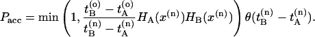
H-U Transition. The F-H transition is followed by the H-U transition: dissolution of the hydrophobic core. Because this transition has a relatively low free-energy barrier, it probably has an unfolding-rate constant in the order of nanoseconds. However, straightforward simulations showed a reasonable stability of the H and U states. We concluded that the unfolding is therefore too slow to study straightforwardly and decided to study this transition with TPS. The time slice separation was 1 ps with a shot length of l = 100 ps. The stable-state criteria are given in Table 1. The path sampling is very efficient, and a typical path ensemble collection is given in Fig. 2. In Fig. 2f, the paths are plotted in the (R_g, N_wat) plane together with a free-energy contour obtained from straightforward MD simulations. Inspection of the pathways reveal that, during the H-U transition, the R_g has to increase first to ≈6 Å before the number of solvent molecules can rise. This is probably due to the fact that the hydrophobic residues must be a minimum distance apart to make enough space for the solvent. This behavior is shown in Fig. 4, where several snapshots along a H-U unfolding path are depicted together with the solvent structure. These snapshots show that, when the hydrophobic core is intact, there is a ring-shaped hydrogen-bond network around the core. When the hydrophobic residues are moving apart, this hydrogen-bond network is rearranged and the water moves in.

Fig. 4.

Solvent structure around the transition states of the H-U paths. A ring of hydrogen bonds is broken, and solvent molecules occupy the space between the hydrophobic groups. The last structure is a transition state. The solvent is depicted as triangles connected with dotted lines for hydrogen bonds. The space-filling molecules are the waters used for the N_wat parameter.

Rate Constants

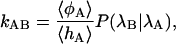
Transition Interface Sampling (TIS). Conventional methods such as the Bennett–Chandler technique (1, 2) are not efficient for calculating the rate constant for complex transitions. If the order parameters used to estimate the barrier do not correspond to the reaction coordinates, the constraining techniques used to calculate the free-energy barrier (such as umbrella sampling) can lead to unrealistic free-energy profiles and extreme hysteresis. Even if the free-energy barrier is properly sampled, the barrier will likely be lower than the real barrier, and the calculation of a statistically accurate transmission coefficient will be exceedingly difficult (8, 32). Within the TPS framework, however, it is possible to calculate the rate constant accurately by determining the reversible work for constraining the paths to end in the final product region. Recently we presented the more efficient TIS method (32), which will be used for the β-hairpin. In short, the TIS method calculates the flux to leave a stable state and, subsequently, the conditional probability to reach the final state provided that the boundary describing the initial state has been crossed. The basis of the method is the equation

[1]

where the forward rate constant k_AB is separated into two factors. The first factor is the flux 〈φ_A〉/〈h_A〉 to leave region A, and the second factor is the conditional probability P(λ_B|λ_A) to reach region B (defined by order parameter λ_B) once the surface λ_A defining region A is passed. The flux factor can be measured by starting an MD simulation in stable-state A. The interface λ_A will be crossed often, resulting in a statistically accurate value for the first factor. In contrast, the value of P(λ_B|λ_A) is very low for a high barrier and cannot be measured directly. The statistics can be improved considerably by using a biased sampling scheme. By sampling paths with the constraint that it comes from region A, crosses an interface λ_i, and then either goes to B or returns to A, we can measure the probability to reach values of λ larger than λ_i. These probabilities are binned in a histogram, and after having performed several simulations for different interfaces λ_i, these histograms are joined into a master curve, from which the value of P(λ_B|λ_A) can be extracted. A more detailed description of TIS can be found in ref. 32.

Results and Discussion. The F-H transition is presumably the rate-determining step in the unfolding (18–20), but because F is actually a metastable state and reaches N within nanoseconds, we calculate the rate constant for the N-H transition. We measured P(λ_B|λ_A) by conducting TIS simulations for several interfaces λ_i. The order parameter for the interfaces was the distance R_OH, a continuous variable distinguishing the stable states quite well. Stable-state definitions are the same as in Table 1, and the values for the interfaces were λ_i = R_OH = 14, 16, 20, 23, 28, 32, 36, 40, and 44. For each interface, we sampled a few hundred paths. From the resulting master curve shown in Fig. 5 Left, it follows that the probability P(λ_B|λ_A) = 1.1 × 10^–5. The flux term in Eq. 1 can be measured directly from an MD simulation of the N state and is ≈20 per ns. The total rate constant at 300 K for unfolding is then 0.20 μs^–1, in reasonable agreement with the experimental result k = 0.17 μs^–1 (13, 14). The folding rate can be deduced from the equilibrium constant K = k_AB/k_BA. Experiments show that, at 300 K, the equilibrium constant is almost unity; hence, the folding-rate constant will equal the unfolding rate (13).

Fig. 5.

(Left) Crossing probability P(λ|λ_A) for the F-H transition as a function of λ = R_OH. This function clearly shows a plateau, indicating that the H state has been reached. (Right) Crossing probability P(λ|λ_A) for the H-U transition as a function of λ = d_min.

The TIS results indicate that there is a high free-energy barrier between the F and H states, in apparent disagreement with the 3–4 kT found in the free-energy landscapes of ref. 25. The discrepancy is caused by an overlap between the F and H states, thus apparently lowering the barriers in the projection on the N_hb, R_g plane.

The error in our calculated rate constant can be quite large because the error in the probability P(λ_B|λ_A) grows exponentially. Nevertheless, inspection of Fig. 5 suggests that this error is at a factor of ≈2. The value of the rate constant also agrees with previous theoretical estimates in implicit solvent by Zagrovic et al. (19). One might conclude that the solvent apparently does not play an important role in the folding; but if that is the case, it probably holds only for the rate-limiting step. The solvent clearly plays a role in the dissolution of the hydrophobic core.

We also calculated the rate constant for the H-U process with TIS. We chose λ = d_min as an order parameter because that seemed to be the most sensitive parameter for the transition. Values for interfaces were λ_i = d_min = 3, 4, and 5. From the master curve in Fig. 5 Right, it follows that the probability P(λ|λ_A) = 1.6 × 10^–2. The flux term was obtained directly from an MD simulation of the H state and turned out to be 40 ns^–1. The total rate constant was 0.6 ns^–1, ≈3 orders of magnitude faster than the F-H transition. This confirms that the folding obeys two-state behavior as well as the notion that the F-H transition is the rate-limiting step in the unfolding process and also the observation by several authors that the H state is not extremely stable. Garcia and Sanbonmatsu (24) and Zhou et al. (25) claim that the H state is not well populated and hence has a high free-energy relative to the F and U states. Straightforward MD simulation showed reasonable stability of the H state, but when continued for several nanoseconds more, the unfolding takes place spontaneously, in line with the calculated rate constant.

Appendix: The TPS Algorithm

TPS algorithms using the deterministic shooting algorithm run into problems for long deterministic trajectories over rough energy landscapes that cause the process to behave more diffusively. This type of diffusive transition is found in, for example, crystal nucleation or, as in this article, protein folding. The original shooting method fails for such barriers, because when the path is becoming too long, the old and the new trajectories will have diverged completely before the other basin of attraction is reached. In that case, a small change in momenta will cause the forward as well as the backward trajectory to return to the same stable region. These nonreactive trajectories will make up the majority of the trial moves. We can improve the efficiency dramatically by making use of a stochastic TPS scheme (31). In the stochastic TPS scheme, one can accept a forward or backward shot independent of each other (8). Stochastic trajectories are obtained by coupling the system to a heat bath with the Andersen thermostat (34). The frequency of the coupling is chosen low enough to keep the dynamics virtually deterministic to have realistic mechanisms and rate constants while still having a quick but controlled divergence from the old path. Energy is kept constant by rescaling the kinetic energy of the system back to the old value after having obeyed constraints (RATTLE algorithm; ref. 30).

Further efficiency is obtained by making the path length variable. Because only shots from the barrier itself are useful in stochastic path sampling, it is natural to stop with the integration of the equation of motion when one reaches a stable state, provided that the trajectory is then really committed to a stable state. Alternatively, one can shoot a trial path of a fixed length l starting from a random time slice as long as this length l is longer than the molecular commitment time (8).

The path-sampling algorithm now becomes the following. Start with an initial path connecting A and B (for more details on how to create an initial path see ref. 8). Let be the time just before leaving A and the first time the system enters B on the old path. The barrier is thus between and . Now choose a slice x_t′ between and with a uniform probability.¶ Next, integrate the equations of motion forward and backward in time for a duration of l time slices by using the Andersen thermostat as a stochastic noise generator. This new trial path is now τ = 2l + 1 time slices long. If the trial path still connects A with B, the shot is accepted with a probability

[2]

Here, H_A(x) = 1 if the path visits A and H_A(x) = 0 otherwise, and x denotes the phase-space coordinates of the entire path of length τ. The superscripts o and n refer to the old and the new path, respectively. The step function θ(x) = 1 for x > 0 and θ(x) = 0 otherwise and ensures that B is reached after A. The last slice of the backward trajectory is renamed time slice 0, the last one of the forward trajectory is renamed time slice 2l, and the shooting point x_t′ becomes time slice l. If the backward path reaches A but the forward shot fails to visit B, the forward trajectory is rejected and the old forward part is retained. The old backward path from t = t′ to t = t′ – lΔt is then replaced (Eq. 2) by the new backward trajectory and accepted with the acceptance rule. Similarly, if the forward path reaches B but the backward shot fails to visit A, the forward trajectory is substituted from t = t′ to t = t′ + lΔt and accepted with the acceptance ratio described above. The new path is shifted such that the first slice is at t = 0. Detailed balance is conserved in this scheme.

During the sampling the path, length fluctuates but remains bounded because of the fraction inside the acceptance probability (Eq. 2). Also, we do not have to perform shifting moves because these Monte Carlo moves have no effect on the ensemble, in contrast to previous TPS studies. The enhancement of statistics that the shifting move provides should be done afterward in the analysis.

References

- 1.Chandler, D. (1978) J. Chem. Phys. 68, 2959–2970. [Google Scholar]
- 2.Bennett, C. H. (1977) in Algorithms for Chemical Computations, ed. Christoffersen, R. (Am. Chem. Soc., Washington, DC), pp. 63–97.
- 3.Dellago, C., Bolhuis, P. G., Csajka, F. S. & Chandler, D. (1998) J. Chem. Phys. 108, 1964–1977. [Google Scholar]
- 4.Dellago, C., Bolhuis, P. G. & Chandler, D. (1998) J. Chem. Phys. 108, 9236–9245. [Google Scholar]
- 5.Bolhuis, P. G., Dellago, C. & Chandler, D. (1998) Faraday Discuss. 110, 421–436. [Google Scholar]
- 6.Dellago, C., Bolhuis, P. G. & Chandler, D. (1999) J. Chem. Phys. 110, 6617–6625. [Google Scholar]
- 7.Bolhuis, P. G., Chandler, D., Dellago, C. & Geissler, P. L. (2002) Annu. Rev. Phys. Chem. 54, 291–318. [DOI] [PubMed] [Google Scholar]
- 8.Dellago, C., Bolhuis, P. G. & Geissler, P. L. (2002) Adv. Chem. Phys. 123, 1–78. [Google Scholar]
- 9.Dellago, C., Bolhuis, P. G. & Chandler, D. (2000) Proc. Natl. Acad. Sci. USA 97, 5877–5882. [DOI] [PMC free article] [PubMed] [Google Scholar]
- 10.Bolhuis, P. G. & Chandler, D. (2000) J. Chem. Phys. 113, 8154–8160. [Google Scholar]
- 11.Blanco, F. J., Rivas, G. & Serrano, L. (1994) Nat. Struct. Biol. 1, 584–590. [DOI] [PubMed] [Google Scholar]
- 12.Blanco, F. J. & Serrano, L. (1995) Eur. J. Biochem. 230, 634–649. [DOI] [PubMed] [Google Scholar]
- 13.Muñoz, V., Thomson, P. A., Hofrichter, J. & Eaton, W. A. (1997) Nature 390, 196–199. [DOI] [PubMed] [Google Scholar]
- 14.Muñoz, V., Henry, E. R., Hofrichter, J. & Eaton, W. A. (1998) Proc. Natl. Acad. Sci. USA 95, 5872–5879. [DOI] [PMC free article] [PubMed] [Google Scholar]
- 15.Honda, S., Kobayashi, N. & Munekata, E. (2000) J. Mol. Biol. 295, 269–278. [DOI] [PubMed] [Google Scholar]
- 16.Kolinski, A., Ilkowski, B. & Skolnick, J. (1999) Biophys. J. 77, 2942–2952. [DOI] [PMC free article] [PubMed] [Google Scholar]
- 17.Klimov, D. K. & Thirumalai, D. (2000) Proc. Natl. Acad. Sci. USA 97, 2544–2549. [DOI] [PMC free article] [PubMed] [Google Scholar]
- 18.Dinner, A. R., Lazaridis, T. & Karplus, M. (1999) Proc. Natl. Acad. Sci. USA 96, 9068–9073. [DOI] [PMC free article] [PubMed] [Google Scholar]
- 19.Zagrovic, B., Sorin, E. J. & Pande, V. (2001) J. Mol. Biol. 313, 151–169. [DOI] [PubMed] [Google Scholar]
- 20.Pande, V. S. & Rokhsar, D. S. (1999) Proc. Natl. Acad. Sci. USA 96, 9062–9067. [DOI] [PMC free article] [PubMed] [Google Scholar]
- 21.Roccatano, D., Amadel, A., Di Nola, A. & Berendsen, H. J. C. (1999) Protein Sci. 8, 2130–2143. [DOI] [PMC free article] [PubMed] [Google Scholar]
- 22.Ma, B. & Nussinov, R. (2000) J. Mol. Biol. 296, 1091–1104. [DOI] [PubMed] [Google Scholar]
- 23.Eastman, P., Gronbech-Jensen, N. & Doniach, S. (2001) J. Chem. Phys. 114, 3823–3841. [Google Scholar]
- 24.Garcia, A. E. & Sanbonmatsu, K. Y. (2001) Proteins Struct. Funct. Genet. 42, 345–354. [DOI] [PubMed] [Google Scholar]
- 25.Zhou, R., Berne, B. J. & Germain, R. (2001) Proc. Natl. Acad. Sci. USA 98, 14931–14936. [DOI] [PMC free article] [PubMed] [Google Scholar]
- 26.Tsai, J. & Levitt, M. (2002) Biophys. Chem. 101, 187–201. [DOI] [PubMed] [Google Scholar]
- 27.Zhou, R. & Berne, B. J. (2002) Proc. Natl. Acad. Sci. USA 99, 12777–12782. [DOI] [PMC free article] [PubMed] [Google Scholar]
- 28.Kale, L., Skeel, R., Bhandarkar, M., Brunner, R., Gursoy, A., Krawetz, N., Phillips, J., Shinozaki, A., Varadarajan, K. & Schulten, K. (1999) J. Comput. Phys. 151, 283–312. [Google Scholar]
- 29.MacKerell, A. D., Jr., Bashford, D., Bellott, M., Dunbrack, R. L., Jr., Evanseck, J. D., Field, M. J., Fischer, S., Gao, J., Guo, H., Ha, S., et al. (1998) J. Phys. Chem. B 102, 3586–3616. [DOI] [PubMed] [Google Scholar]
- 30.Andersen, H. C. (1983) J. Comput. Phys. 52, 24–34. [Google Scholar]
- 31.Bolhuis, P. G. (2003) J. Phys. Condens. Matter 15, S113–S120. [Google Scholar]
- 32.van Erp, T., Moroni, D. & Bolhuis, P. G. (2003) J. Chem. Phys. 118, 7762–7774. [DOI] [PubMed] [Google Scholar]
- 33.Humphrey, W., Dalke, A. & Schulten, K. (1996) J. Mol. Graphics 14, 33–38. [DOI] [PubMed] [Google Scholar]
- 34.Andersen, H. C. (1980) J. Chem. Phys. 72, 2384–2393. [Google Scholar]