An Efficient Numerical Technique for Bioheat Simulations and its Application to Computerized Cryosurgery Planning

Abstract

As a part of ongoing efforts to develop computerized planning tools for cryosurgery, the current study focuses on developing an efficient numerical technique for bioheat transfer simulations. Our long-term goal is to develop a planning tool for cryosurgery that takes a 3D reconstruction of a target region, and suggests the best cryoprobe layout. Toward that goal, a planning algorithm, termed “force-field analogy,” has been recently presented, based on a sequence of bioheat transfer simulations, which are by far the most computationally expensive part of the planning method. The objective in the current study is to develop a finite difference numerical scheme for bioheat transfer simulations, which reduces the overall run time of computerized planning, thereby making it clinically relevant. While the general concept of variable grid size and time intervals is not new, its application to the phase change problem of cryosurgery is the unique contribution of the current study.

1. Introduction

Simulation of heat transfer problems involving phase change is of great importance in the study of thermal injury to biological systems. One of the most relevant examples is cryosurgery, which is the intentional destruction of undesired biological tissues by freezing [1]. Modern cryosurgery is frequently performed as a minimally-invasive procedure, with the application of a large number of cooling probes (cryoprobes), in the shape of long hypodermic needles, strategically located in the area to be destroyed (the target region) [2]. Here, the reconstruction of the target region, as well as monitoring of the freezing process, must be performed by means of imaging devices such as ultrasound or MRI [3–6].

The clinical application of cryosurgery is not without technical difficulties, some of which are related to planning and control of a large number of cryoprobes, while others are related to the quality and limitations of imaging techniques. The long-term benefit of cryosurgery is not only affected by those technical difficulties, but also by the specific thermal history forced upon the tissue, the unique response of the tissue to low temperature exposure, and possibly the presence of drugs that sensitize that tissue to injury at low temperatures [7].

Since temperature can be measured only at discrete points in the target region, simulation of heat transfer is an extremely useful tool in developing and improving cryosurgical techniques [8–11]. Here, heat transfer simulations can be calibrated with temperature measurements in the target tissue for the purpose of parametric estimation of tissue properties [12]. Heat transfer simulations can also assist in evaluating the certainty in temperature measurements, as has been demonstrated for the application of hypodermic thermocouples during cryosurgery [13]. Heat transfer simulations can also be used to augment imaging in real time, by identifying specific temperature thresholds within the frozen region [14]. However, one must bear in mind that the quality of those simulations relies on the certainty of the available values of the thermophysical properties of the tissue [15].

As a part of an ongoing project to develop an automated planning tool for cryosurgery, the current study is aimed at developing a numerical scheme which significantly reduces the heat transfer simulation run time; the duration of simulation has been identified as a critical factor in making that tool clinically relevant. Prior work on this ongoing project focused on the development of a force-field analogy technique, which executes a series of heat transfer simulations and automatically relocates cryoprobes between every two consecutive runs, until an optimum cryoprobe layout is found [16,17]. Prior work also included the development of an algorithm to predict the best initial condition for the force-field analogy procedure (termed “bubble-packing”), in order to decrease the number of heat transfer simulations required in the force-field analogy process [18]. Finally, prior work included the development of the cryoheater, a self-controlled electrical heater, which helps to limit freezing injury to the target region [19]. Consistent with previous work, the new technique is demonstrated on a geometrical model of a prostate, where prostate cryosurgery is a common minimally-invasive procedure.

2. Mathematical Formulation

Bioheat transfer in this study is modeled with the classic bioheat equation [20]:

$$C=\frac{\partial T}{\partial t}=\nabla \cdot (k\nabla T)+{\stackrel{.}{w}}_b{C}_b(T_b-T)+{\stackrel{.}{q}}_{met}$$ (1)

where C is the volumetric specific heat of the tissue, T is the temperature, t is the time, k is the thermal conductivity of the tissue, ẇ_b is the blood perfusion volumetric flow rate per unit volume of tissue, C_b is the volumetric specific heat of the blood, T_b is the blood temperature entering the thermally treated area, and q̇_met is the metabolic heat generation. Numerous scientific reports have been published studying the mathematical consistency and validity of the above classic equation, while exploring various alternatives (for example, see Charny [21] and Diller [8]). It is assumed in the current study that a more advanced model of bioheat transfer will not warrant higher accuracy in the cryosurgery simulation, will involve greater mathematical complications, and is deemed unnecessary in the current study. Note that metabolic heat generation is typically negligible compared to the heating effect of blood perfusion, and is neglected in this study [22]. Table 1 lists typical values of the thermophysical properties used in the current study. It is assumed in this study that the specific heat is an effective property within the phase transition temperature range of −22°C to 0°C (if the tissue is first order approximated as an NaCl solution), where a detailed discussion about the application of the effective specific heat to phase change problems is given by Rabin and Korin [23].

Table 1.

Representative thermophysical properties of biological tissues used in the current study [17].

Thermophysical Property	Value
	0.5	273K < T
Thermal conductivity, k, W/m-K	15.98 – 0.0567×T	251K < T < 273K
	1005×T − 1.15	T< 251K
	3.6	273K < T
Volumetric specific heat, C, MJ/m3-K	880 – 3.21×T	265K < T < 273K
	2.017×T – 505.3	251K < T < 265K
	0.00415×T	T < 251K
Blood perfusion, wbCb, kW/m3-K	40

The new numerical scheme is a modification of a previous numerical scheme [22], which has been developed for cryosurgery simulations. The modification concerns variable grid spacing and time intervals. The term “variable grid” is used in the context of distinct regions in the domain possessing different grid sizes and not merely changing the space intervals in a specific direction across the entire grid, as illustrated in Fig. 1. The rationale for using a variable grid is that a fine grid is necessary only in regions characterized by steep temperature gradients (close to cryoprobes, for example), while a coarser grid can be applied in regions characterized by more moderate temperature gradients. Optimizing the grid in accordance with the temperature distribution can reduce the overall number of grid points and thereby reduce the number of computer operations over a given time interval. Furthermore, due to stability criteria (discussed below), a larger grid size allows for longer time intervals. Thus, simulation run time for variable grid solutions can be further shortened if the thermal history at any given grid point progresses in accordance with its own unique time interval, associated with the local stability criterion. The application of the current numerical scheme takes advantage of this effect.

Figure 1.

Schematic illustration of a variable grid of 1:3 ratio in the 2D case, representative of a prostate cryosurgery; the thermal resistance network used for numerical simulations is illustrated on the right. The progression of the freezing front along arrows A, B, and C, for a special case of planning, is presented in Fig. 4.

Equation (1) can be rewritten in a finite difference form [22]:

$$\begin{array}{r}{T}_{i,j,k}^{p+1}=\frac{\mathrm{\Delta }t}{\mathrm{\Delta }{V}_{i,j,k}[C_{i,j,k}+{({\stackrel{.}{w}}_b{C}_b)}_{i,j,k}\mathrm{\Delta }t]}\sum _{l,m,n}\frac{T_{l,m,n}^p-T_{i,j,k}^p}{R_{l,m,n-i,j,k}}\\ +\frac{\mathrm{\Delta }t\hspace{0.17em}[{({\stackrel{.}{w}}_b{C}_b)}_{i,j,k}{T}_b+{({\stackrel{.}{q}}_{met})}_{i,j,k}]+C_{i,j,k}\hspace{0.17em}{T}_{i,j,k}^p}{C_{i,j,k}+{({\stackrel{.}{w}}_b{C}_b)}_{i,j,k}\hspace{0.17em}\mathrm{\Delta }t}\end{array}$$ (2)

where i,j,k and l,m,n are space indexes, p is a time index, ΔV is an element volume associated with a grid point, Δt is a time interval, and R is the thermal resistance to heat transfer by conduction between node i,j,k and its neighbor l,m,n. Equation (2) is rather general, and its formulation is independent of the coordinate system. For a regular Cartesian grid, the thermal resistance to heat conduction can be simply presented as:

$$R_{l,m,n-i,j,k}={\left[\frac{\mathrm{\Delta }\eta }{2kA}\right]}_{l,m,n}+{\left[\frac{\mathrm{\Delta }\eta }{2kA}\right]}_{i,j,k}$$ (3)

where the length Δη is the space interval in the direction of interest, and A is the representative cross-sectional area perpendicular to the direction of heat flow.

Figure 1 schematically illustrates a 2D domain, representative of a cross-section during prostate cryosurgery. For demonstration purposes, Fig. 1 includes two grid sizes, a general, coarse grid, and a fine grid around the cryoprobes and the urethra; the urethra runs through the prostate, and is warmed by a special heater during cryosurgery.

Figure 1 (right) also presents a schematic illustration of the thermal resistance network around a grid point in the fine grid region and the resistance network at the transition region from fine to coarse grids. Figure 1 presents a coarse-to-fine grid ratio of 1:3, which corresponds to a grid points ratio of 1:9 in 2D. These ratios illustrate the potential run time reduction by varying grid size. For efficiency in computation in the current study, only an integer is assumed for the grid ratio. The thermal resistances across the cryoprobe wall and across the urethral warmer wall are assumed to be negligible in the current study, and a uniform temperature distribution is therefore assumed across these thermal elements.

Stability analysis indicates that the maximum allowable time interval at any grid point is:

$$\mathrm{\Delta }t\le {\left[\frac{{(C\mathrm{\Delta }V)}_{i,j,k}}{\sum _{l,m,n}\left(1/R_{l,m,n-i,j,k}\right)}\right]}_{min}$$ (4)

where increased blood perfusion has been shown to increase stability for the scheme presented in Eq. (2) [22]. It can be seen from Eq. (4) that the maximum allowable time step is proportional to square of the space interval. While the maximum allowable time interval may vary between grid points, due to variation in material properties, its variation between fine-to-coarse grids (Fig. 1) is expected to be far more dramatic.

For practical reasons, it is efficient to select variable time intervals so that the ratio of longer to shorter time intervals equals an integer. In the current study, the maximum allowable time interval for the finest grid is evaluated first. The same time interval is used for all grid points in the finest grid regions. Next, the maximum allowable time interval for the coarse grid is calculated. Finally, the latter time interval is shortened to be the product of the shorter time interval and the truncated ratio of the coarse to the finest grid time intervals.

The concept of variable grid using multiple levels has already been presented in the context of control volume numerical techniques, with an example of a grid ratio of 1:2 between every two consecutive levels [24]. In the current study however--where the numerical scheme is tailored for the specific application of heat transfer with phase change during cryosurgery--only two grid levels are selected. As discussed below, a grid ratio higher than 1:2 was found to be efficient for the specific case of cryosurgery, bringing simulation to a clinically relevant run time for the purpose of cryosurgery planning. However, if more than two grid levels are used for cryosurgery, the efficiency of grid ratios higher than 1:2 must be revisited.

3. Application to Computerized Planning of Cryosurgery

While the numerical scheme presented above is quite general, the main objective for its development is to accelerate numerical simulations of cryosurgery, in order to make previously established planning algorithms practical [17,18]. The objective in cryosurgery is to maximize freezing damage internal to the target region while minimizing freezing damage external to the target region. Consistent with prior work, a target region area is defined by the outer contour of the prostate, excluding the urethra (Fig. 1).

Consistent with clinical practice, it is assumed that cryoinjury is associated with the thermal history of the tissue. While the concept of the so-called “lethal temperature” is widely accepted by clinicians as the threshold temperature below which maximum cryoinjury is achieved, the parameter monitored during cryosurgery is most frequently the freezing front, using ultrasound imaging, which is likely to be associated with the isotherm of 0ºC (i.e., the onset of crystal formation). Since currently accepted values for lethal temperature are in the range of −50ºC to −40ºC [7,10], and since cryoinjury is assumed to progress gradually between the onset of crystal formation and the lethal temperature threshold, the isotherm of −22ºC has been selected for planning in this study, splitting this temperature range associated with tissue injury by about half (note that −22ºC is also the lower boundary for phase transition). The optimal match of that isotherm with the contour of the target region is the objective of planning, splitting the undesired effects of excessive cryoinjury external to the target region, and incomplete cryoinjury internal to the target region. Nevertheless, the isotherm value of −22ºC is selected in the current work for demonstration purposes only, while its actual value is left to the decision of the cryosurgeon; the planning algorithms presented previously are independent of the value of the optimization isotherm.

The objective function of planning can be formulated as [17]:

$$G=\underset{V}{\int }w\hspace{0.17em}dV\hspace{0.17em}\hspace{0.17em}\hspace{0.17em};\hspace{0.17em}\hspace{0.17em}w=\{\begin{array}{ccc}1& -{22}^{°}C<T& \text{interior to the target region}\\ 0& T\le -{22}^{º}C& \text{interior to the target region}\\ 1& T\le -{22}^{º}C& \text{exterior to the target region}\\ 0& -{22}^{º}C<T& \text{exterior to the target region}\end{array}$$ (5)

where G is the value of the target function (also termed a “defect function”), V is the volume of the domain under consideration, and ω is a spatial weight function determined by the local temperature distribution. In the course of integration in the current study, the temperature distribution of the coarse grid region is interpolated, to generate a uniform distribution of temperature data in the domain; bilinear and trilinear interpolations were used for the 2D and 3D cases, respectively.

The simulation starts with a maximum objective function value, which equals the entire target region (i.e., maximum internal defect). The overall defect decreases with the progression of simulation, as a larger portion of the target region falls bellow the isotherm threshold of planning. Eventually, an excessive frozen volume develops outside of the target region (external defect), which leads to a gradual increase of the overall defect size. The bioheat transfer simulation is terminated at the point of minimum defect, and the planning algorithms presented previously [17,18], process the resulting temperature field to automatically suggest a better cryoprobe layout. Hence, the objective function, G, is used in two different ways: to indicate when to terminate a bioheat transfer simulation for a specific cryoprobe layout (when G reaches a local minimum), and to indicate when the best cryoprobe layout is found (when G reaches a global minimum). That process of iterative planning, however, is outside of the scope of the current study.

Since the size of the overall defect is dependent on the cryoprobe layout, and is not known a priori, the time point of minimum defect must be located within the defect history. Thus, the simulation time must surpass the point of minimum defect before a minimum value is identified. In the current study, the minimum defect is continually sought within the last 30 seconds of the defect history, a time window which has proven to be adequate in the current study. Results for the defect region are presented as a percentage of the size of the target region.

4. Results and Discussion

The new numerical scheme has been analyzed in 1D, 2D, and 3D, to study its various characteristics. The prostate model used in the 2D and 3D cases has been reconstructed from a set of ultrasound images which were made available by the Robarts Imaging Institute, London, Ontario, Canada [25] for the purpose of the current study. The prostate images were segmented manually at our laboratory in order to reconstruct a full 3D target region. Since the ultrasound image data was not obtained during cryosurgery, the urethral warmer was absent from imaging, and a 6 mm in diameter urethral warmer was assumed along the centerline of the imaged urethra. Consistent with clinical practice, the urethral warmer is simulated as a heat source, providing a constant temperature of 37°C.

The simulated cryoprobes in the current study are assumed to cool from an initial temperature of 37ºC down to −145ºC, at a constant cooling rate of 6ºC/sec, and hold a constant temperature of −145ºC thereafter. This relatively high cooling rate is typical of the Joule-Thomson effect-based cryoprobes, operating with Argon gas [17].

4.1 Analysis of the 1D Case

The objective for the 1D analysis was to identify the appropriate grid size in areas of steep temperature gradients; this analysis was focused on uniform grid intervals. Figure 2 presents the location of a freezing front defined by the 0ºC isotherm, which represents the upper boundary of the phase transition temperature range (Table 1).

Figure 2.

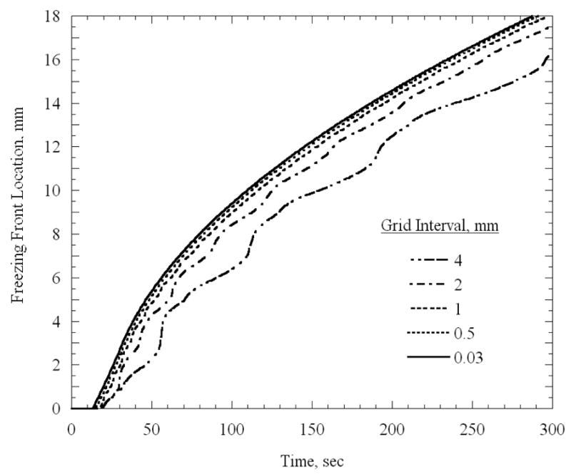
Freezing front location as a function of time for a 1D uniform grid case, which represents the upper boundary of phase transition, 0ºC.

It can be seen from Fig. 2 that the freezing front location converges with the decrease in grid size, where the grid size of 0.03 mm is considered as the reference solution in the current analysis. At the end of the five minute simulations presented in Fig. 2, the difference between the reference solution and the solutions based on 0.5 mm, 1 mm, 2 mm, and 4 mm is 0.6%, 1.8%, 4.8%, and 11.4%, respectively. A 1.8% level of accuracy is assumed adequate for the purpose of the current study, and the 1 mm grid interval was selected for the finest grid in the 2D and 3D analyses presented below.

4.2 Analysis of the 2D Case

The main objective of the 2D analysis is to compare results based on the variable grid scheme with the benchmark solution suggested by Rabin and Shitzer [22]. The largest cross-sectional area from the 3D reconstructed prostate was used for the 2D analysis, as illustrated in Fig. 1. The fine grid is based on 1 mm spacing in both directions. Each cryoprobe is represented as a square 1 mm × 1 mm region, which conforms to the finest grid; its perimeter is equivalent to that of a circular cryoprobe having a diameter of 1.3 mm. A 1 mm grid is also selected around the urethra. The 2D analysis focuses on a case study of a coarse-to-fine grid ratio in the range of 1:2 to 1:5. The simulated cross-sectional area, including the prostate and surrounding healthy tissues, is 120 mm × 120 mm. An adiabatic boundary condition was imposed on the entire region. Temperature changes of less than 0.03°C were observed at that boundary, at the end of simulation, which indicates that the region can be considered as infinite for heat transfer calculations.

Figure 3 presents the temperature field at the point of minimum defect, for the cryoprobe layout illustrated in Fig. 1, and for the case of a uniform grid. The ten-cryoprobe configuration was determined using the force-field analogy optimization technique [16]. A good agreement can be seen between the −22°C isotherm and the target region contour, yielding a relatively small defect value of 3.9%.

Figure 3.

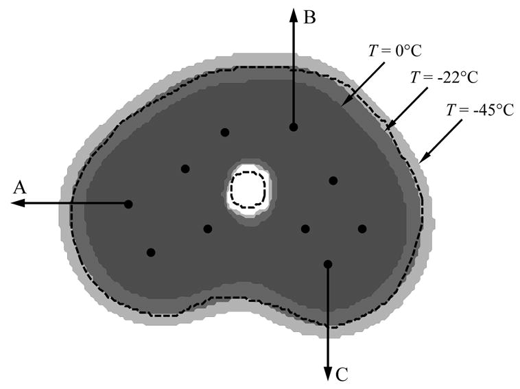
Temperature regions at the point of minimum defect for the grid presented in Fig. 1, where the external dashed line represents the prostate outer contour, the inner dashed line represents the urethral warmer, and the dark, medium, and light gray represent areas with temperatures below −45ºC, −22ºC, and 0ºC, respectively. The progression of the freezing front along the three arrows is presented in Fig. 4.

Figure 4 presents the freezing front location along representative lines marked with A, B, and C in Fig. 3, using a variable grid, as illustrated in Fig. 1. Here, the freezing front is represented by the 0°C isotherm, which is the upper boundary of phase transition. Consistent with the 1D results, the freezing front propagates slower through a larger grid. From Fig. 4(a) for example, it can be seen that at five minutes, the freezing front location is 11.8 mm, 11.4 mm, 11.0 mm, 10.4 mm, and 9.5 mm, for the grid ratios of 1:1, 1:2, 1:3, 1:4, and 1:5, respectively. For the 1:2 to 1:5 cases, these location differences represent 3.4%, 7.3%, 11.9%, and 19.5% error from the 1:1 uniform grid solution. For the 1:2 and 1:3 solutions, the corresponding percentage differences decrease over time, but their absolute difference remains about the same with time. For the 1:4 and 1:5 solutions, much larger fluctuations are present over time, indicating less accurate solutions. Similar results are observed in Figs. 4(b) and 4(c), which are consistent with results of the 1D case presented in Fig. 2.

Figure 4.

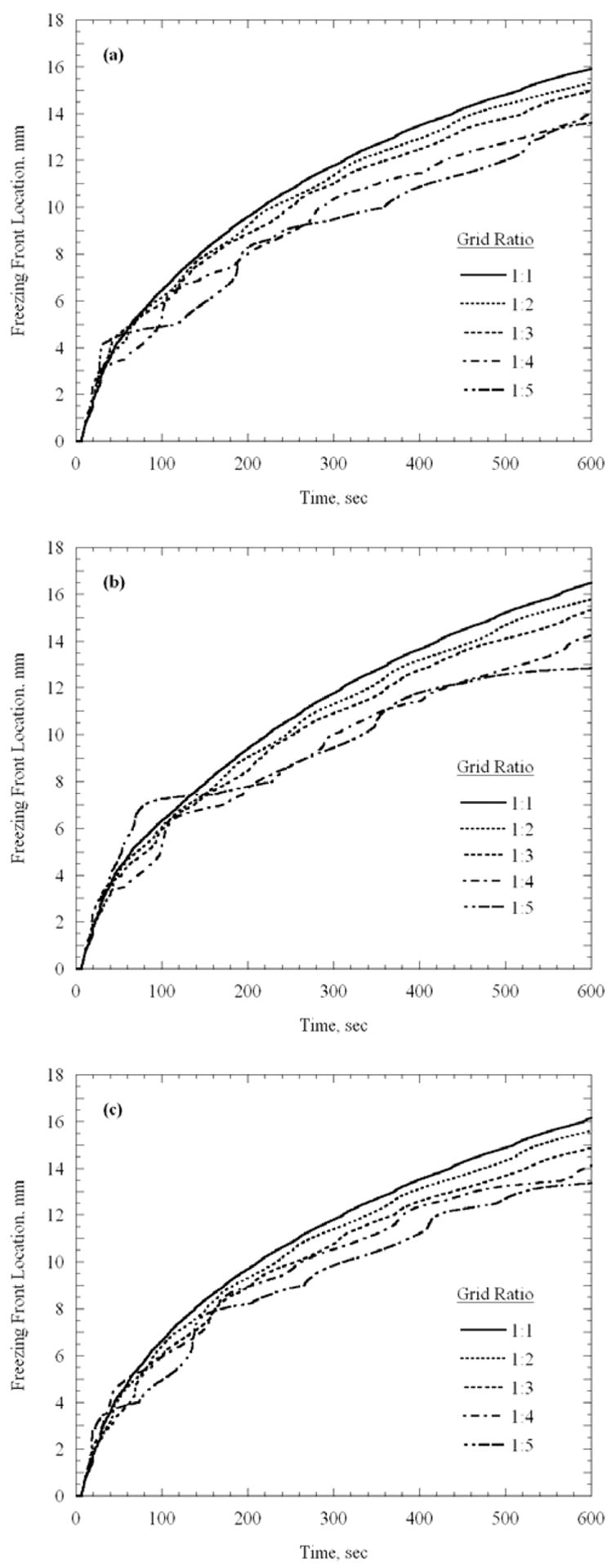
Propagation of the 0ºC isotherm (upper boundary of phase transition) along the lines illustrated in Figs. 1 and 3: (a) line A, (b) line B, and (c) line C.

In order to place the above numbers in the appropriate cryosurgical context, it is noted that an uncertainty of 1 mm in identification of the freezing front location can be considered reasonable with a high quality ultrasound device. Another significant effect that affects the outcome of cryosurgery planning is uncertainty in thermophysical properties, and its propagation into the current heat transfer simulation. For example, the uncertainty associated with thermal conductivity is typically in the range of 15%, and the uncertainty associated with thermal diffusivity is typically in the range of 10% to 20%, while the actual blood perfusion rate in cryogenic applications remains largely unknown [15]. These uncertainties lead to uncertainty in the prediction of the freezing front location, which can easily exceed 10% after three minutes of simulation [15]. It follows that, for the clinical application of cryosurgery planning, it reasonable to aim for a numerical solution uncertainty equal to or less than uncertainty from other sources.

A consequence of the error presented in Fig. 4 is the evident time lag in estimating the freezing front location; this time lag increases with the increasing grid ratio. However, it should be remembered that the agreement between the target region and the contour defined by the isotherm for optimization is to be evaluated at the point of minimum defect, rather than at any specific simulated time. To stress this point, Fig. 5 presents the isotherm of −22ºC at the time when minimum defect is reached for the 1:1 and 1:3 grid ratio cases. While the minimum defect for the 1:1 and 1:3 cases is found at 5.3 min and 5.7 min, respectively, a very good agreement between the target region and the optimization isotherm is evident. The minimum overall defect region for the 1:1, 1:2, 1:3, 1:4, and 1:5 cases are 3.9% 4.2%, 4.1%, 5.1%, and 6.0%, respectively.

Figure 5.

Representation of the isotherm −22ºC at the time of minimum defect, for the grid ratios of 1:1 and 1:3.

Results presented in the current study were obtained using a cryosurgery simulator prototype, written with C++, implemented with Visual Studio, and optimized for run time. Run time comparison for the case illustrated in Fig. 1, on a 3.4 GHz Pentium 4 machine, with 512 MB of memory and 800 MHz front side bus yielded 50 sec, 5.5 sec, 4.2 sec, 4.5 sec, and 5.5 sec for grid ratios of 1:1, 1:2, 1:3, 1:4, and 1:5, respectively. It follows that using the variable grid reduces run time by an order of magnitude for the 2D case. An interesting observation is that the grid ratios of 1:4 and 1:5 require longer run time, which corresponds to the increased number of small grid points needed around the cryoprobes to match the relatively large coarse grid at further distances.

For comparison purposes, two additional 2D bioheat transfer simulations were executed using the finite element commercial code ANSYS 8.1; each simulation included ten cryoprobes. The first simulation was executed with a uniform mesh of 1 mm × 1 mm, over a rectangular domain of the same size as that used for the new finite difference solution. The second simulation was executed using a variable mesh, automatically generated by ANSYS, incorporating a finer mesh near the cryoprobes, and having an average element size of 11.4 mm². The average area associated with a given grid point in the finite difference numerical scheme based on a 1:3 grid ratio is under 9 mm², where a combination of 1 mm² and 9 mm² areas are used. This area difference between the ANSYS solution and the finite difference solution gives an advantage to ANSYS in terms of simulation run time in the current comparison. The time step sizes for the ANSYS simulations were set such that the numerical error associated with each of the solutions was comparable to the error of the respective finite difference solutions. Plane55 elements were used in ANSYS simulations to model heat conduction, and Mass71 elements were added to model the blood perfusion heating effect. ANSYS simulations were executed on the same machine used for the finite difference simulations described above. For the uniform grid case, the “performance ratio”, defined as the ratio of cryosurgery simulated time to machine run time, was found to be 1.02 and 3.35, for ANSYS and for the finite difference solution, respectively. For the variable grid case, performance ratios of 4.8 and 40.5 were found for ANSYS and for the finite difference numerical scheme, respectively. In the latter case, the new numerical technique has proven to be an order of magnitude faster than ANSYS. The performance ratio difference is expected to be more dramatic in 3D than in 2D, which further justifies the use of the new numerical solution over ANSYS.

4.3 Analysis of the 3D Case

The process of planning in 3D is illustrated in Fig. 6. Figure 6(a) presents a reconstruction of the prostate, the urethra, cryoprobes already inserted in the prostate, and a cryoprobe placement grid, which is a flat plate with a grid of holes, commonly used by cryosurgeons to assist in cryoprobe placement. Figure 6(b) presents the prostate procedure from a different angle, in which the prostate volume with temperatures below −22ºC is illustrated in dark gray. Two representative cross-sections of the target region, and the resulting temperature field (at a depth of Z₁ and Z₂, Fig. 6(b)), are presented in Fig. 6(c). The resulting defect areas are presented in Fig. 6(d), which are continually integrated over the entire volume in the course of simulation.

Figure 6.

Illustration of the process of cryosurgery simulation: (a) reconstruction of the prostate from ultrasound images, including the urethra, and illustration of the placement grid; (b) 3D representation of the isotherm for optimization (−22ºC in the current study), when the overall defect reaches a minimum value; (c) illustration of temperature regions in two representative cross-sections; (d) translation of the temperature regions into defects.

The simulated domain size bears a direct impact on simulation run time. An underlying assumption in this study is that the body can be modeled as an infinite domain compared to the prostate. Since prostate size may vary between patients, the domain size for simulation was selected proportional to the prostate size, where the coefficient B₁ represents the ratio of the simulation area on the x-y plane to the largest prostate cross-sectional area on the same plane, and B₂ represents the ratio of the length of the simulated region to the maximum length of the prostate (in the z direction). The temperature at the boundary of the entire domain, , was held constant and equal to the initial temperature, while the overall heat loss through the domain boundary was computed as:

$$q_{loss}=-\underset{\mathrm{\Omega }}{\int }k\frac{\partial T}{\partial \widehat{n}}d\mathrm{\Omega }$$ (6)

where n̂ is the normal to the boundary. The total heat generation in the domain due to blood perfusion was computed as:

$$q_{bp}=\underset{V}{\int }{\stackrel{.}{w}}_b{C}_b(T_b-T)dV$$ (7)

The simulated domain can be assumed to be infinite from heat transfer considerations if q_loss is at least two orders of magnitude smaller than q_bp, and therefore can be negligible. For the reconstructed prostate in Fig. 6, having dimensions of 75 mm × 53 mm × 67 mm, and for the worst case scenario of ten cryoprobes, having a length of 30 mm and placed at the edge of the prostate, a conservative value for B₁ was found to be 3.5. Using a separate worst-case scenario, with cryoprobes 50 mm long, placed at the center of the prostate, B₂ was found to be 1.5.

While the numerical scheme is general and can also handle a variable grid scheme in the z direction, it is deemed unwarranted for the current configuration, since all cryoprobes are simulated to be inserted at the same depth. Instead, the space interval in the z direction was varied, as illustrated in Fig. 7. Consistent with results from the 1D analysis, a 1 mm interval was selected near the tip of the cryoprobes. Further parametric studies suggested that a gradual increase of space intervals by a factor of 1.3 between consecutive intervals from the cryoprobes to the domain boundaries, and uniform intervals along the cryoprobes, yield adequate results.

Figure 7.

Schematic illustration of discretization in the z direction.

Results of various parametric studies in 3D are listed in Tables 2–4, where the bubble-packing algorithm [18] has been used to find cryoprobe placement; no further planning optimization was performed. Results for the effect of grid ratio on simulation run time are listed in Table 2; the first 5.1 min are simulated in all cases, which corresponds to the time at which the 1:1 uniform grid size case reached a minimum defect value. Note that two sets of results are listed for the uniform grid solution: the case annotated with “*” refers to a uniform grid in all directions, while the other case refers to a uniform grid in the x-y direction and variable grid intervals in the z direction, as illustrated in Fig. 7. Similarly, all other cases use variable grid intervals in the z direction.

Table 2.

Results of 3D cryosurgery simulations with ten cryoprobes at 305 sec (when the benchmark solution, “^*”, reaches a minimum defect value), where N_f and N_c are the overall numbers of grid points in the fine and coarse grids, respectively, D_T, D_I, and D_E are the total, internal, and external defect volumes, respectively, V₂₂ is the volume of tissue possessing temperatures of no greater than −22ºC, and ΔS is the average difference in freezing front location between the specific solution and the benchmark solution; the volume of the target region is 74.1 cm³.

Grid Ratio	NF	NC	DT, %	DI, cm3	DE, cm3	V22, cm3	ΔS, mm	Run Time, min
1:1*	N/A	654584	22.9	11.0	6.0	63.1	N/A	43.9
1:1	N/A	183594	23.1	10.9	6.3	63.3	0.10	10.7
1:2	1641	48645	23.6	12.2	5.2	61.9	0.35	1.78
1:3	1965	22366	25.2	15.2	3.5	58.9	0.96	0.89
1:4	2885	12923	26.7	17.0	2.8	57.1	1.15	0.88
1:5	4257	8490	28.3	18.8	2.2	55.3	1.75	0.99

^*Benchmark solution with uniform grid of 1mm × 1mm × 1mm

Table 3.

Results of 3D cryosurgery simulations with ten cryoprobes at the time of minimum defect for the specific grid ratio, where D_T, D_I, and D_E are the total, internal, and external defect volumes, respectively, V₂₂ is the volume of tissue possessing temperatures of no greater than -22ºC, and ΔS is the average difference in freezing front location between the specific solution and the benchmark solution; the volume of the target region is 74.1 cm³.

Grid Ratio	Simulated Time, min	DT, %	DI, cm3	DE, cm3	V22, cm3	ΔS, mm	Run Time, min
1:1*	5.1	22.9	11.0	6.0	63.1	N/A	48.6
1:1	5.0	23.1	11.1	6.0	63.0	0.15	11.6
1:2	5.4	23.4	11.2	6.1	62.9	0.22	2.07
1:3	6.4	23.6	10.5	6.9	63.6	0.18	1.22
1:4	6.9	23.3	10.8	6.5	63.3	0.39	1.31
1:5	7.2	23.9	12.0	5.7	62.1	1.03	1.56

^*Benchmark solution with uniform grid of 1mm × 1mm × 1mm

Table 4.

Results of 3D cryosurgery simulations with a grid ratio of 1:3 at the time of minimum defect for the specific number of cryoprobes, where N_F is the number of fine grid points, D_T, D_I, and D_E are the total, internal, and external defect volumes, respectively, V₂₂ is the volume of tissue possessing temperatures of no greater than −22ºC, and ΔS is the average difference in freezing front location between the specific solution and the benchmark solution; the volume of the target region is 74.1 cm³.

Number of Cryoprobes	Simulated Time, min	NF	DT, %	DI, cm3	DE, cm3	V22, cm3	Run Time, min
6	18.5	1507	25.9	13.3	5.9	60.8	3.11
8	8.6	1853	23.7	12.5	6.4	61.7	1.56
10	6.4	1965	23.6	10.5	6.9	63.6	1.22
12	4.7	2599	23.2	11.0	6.2	63.1	1.06
14	3.8	3062	22.7	11.1	5.7	63.0	0.95

It can be seen from Table 2 that the scheme of variable grid intervals in the z direction reduces run time by a factor of four. Furthermore, the scheme of variable grid in x-y direction reduces run time by an additional order of magnitude. It can be seen that the higher grid ratio does not necessarily decrease run time; the reason being that while the total number of grid points decreases with the increasing grid ratio, the number of smaller grid points that require a larger number of time steps increases significantly. Apparently, an optimum exists between the total number of grid points and the number of small grid points. It follows that a ratio higher than 1:3 will not lead to shorter run time, but will lead to higher uncertainty in computer simulation, as discussed in detail above for the 2D case. It can be seen that the 1:3 ratio case results in ten percent error in the defect region volume, and less than seven percent error in the volume defined by the isotherm for optimization, −22ºC.

Consistent with the 2D analysis and Fig. 3, Table 2 lists the average freezing front location along six selected lines, in six directions (±x, ±y, ±z). Consistent with the 2D results, the larger grid ratio leads to a slower progression of the freezing front, with the uncertainty associated with the ratio of the 1:3 case comparable with the uncertainty associated with imaging.

Results listed in Table 3 were obtained from similar cases, the only exception being that each simulation is run until minimum defect is found. The most significant observation is that for planning of cryosurgery, where the optimum cryoprobe layout to match the target region is searched, the different cases presented in Table 3 will lead to a similar layout, with error in the minimum defect area and in the volume enclosed by the −22ºC isotherm in the third significant digit. While the time at which this optimum is found varies significantly, this value alone has no bearing on the current planning.

One of the most significant uncertainties in computer simulation of cryosurgery is the temperature dependency of blood perfusion on temperature [15]. The variation of time to minimum defect decreased considerably when the blood perfusion term was set to zero. Other primary contributors to this error are the smoothing effect of the phase transition on relatively large grid intervals, and the trilinear interpolation--possibly taking into account different gradients on both sides of the phase transition region in a single interpolation operation.

Based on the results listed in Tables 2 and 3, and the related discussion, a grid ratio of 1:3 is assumed adequate for the purpose of developing the computerized planner for cryosurgery. Table 4 lists simulation results for selected numbers of cryoprobes, when each simulation is run to the point of minimum defect. While the number of fine grid points increases with the increasing number of cryoprobes (adversely effecting run time), a larger number of cryoprobes represents higher overall cooling power, which in turn reduces run time by shortening the simulated cryoprocedure (see time to minimum defect in Table 4). The number of coarse grid points is about 22,000 for all cases presented in Table 4. For each case, the simulation run time approaches a clinically relevant duration of 3 min or less. Note that run time is in the range of four to six times faster than the simulated procedure. Both the volume encapsulated by the −22°C isotherm and the minimum defect value are in a close range for all cases, which reflects on the quality of the bubble-packing method used for selecting the layout of cryoprobes [18].

Finally, the discussion turns to the contribution of computer hardware development to computerized planning. Assuming that the computing power available for a given cost doubles every 18 months (consistent with the so-called Moore’s Law [26] ), and assuming that this trend prevails in the near future, it may be concluded that reducing simulation run time by a factor of 40 (corresponding to results listed in Table 3), has an effect similar to eight years of hardware development. Furthermore, with continued CPU development, a 3D simulation, which currently takes one minute, should take less than ten seconds within the next five years. Further reduction in run time could also be obtained through the use of multiple processors, due to the inherently parallelizable nature of the current 3D numerical scheme. For a clinical application, this reduction in run time can enable the incorporation of real time image reconstruction, and the development of complimentary visualization tools.

5. Summary and Conclusions

As a part of an ongoing project to develop an automated tool for cryosurgery planning, the current study presents a numerical scheme that significantly reduces the heat transfer simulation run time, which has been identified as a limiting factor in making this tool clinically relevant. The new numerical scheme is a modification of an early numerical scheme, in which modification is focused on variable grid and time intervals. Prior work focused on the development of a force-field analogy technique, which executes a series of heat transfer simulations, and automatically relocates cryoprobes between every two consecutive runs, until an optimum cryoprobe placement is found. Prior work also included the development of an algorithm to predict the best initial condition for the force-field analogy procedure in order to decrease the number of heat transfer simulations required in the force-field analogy process. Consistent with prior work, the new technique is demonstrated on a geometrical model of a prostate.

Analysis of the numerical technique in 1D suggests that 1 mm intervals can be considered adequate for the fine grid, when only two grid levels are applied in the current study. Analysis in 2D suggests that a ratio of 1:3 between the fine grid and the coarse grid can be considered adequate. Analysis in 3D suggests that a simulated domain containing the prostate model can be considered infinite in the thermal sense, if its cross-sectional area is 3.5 times larger than the largest prostate cross-sectional area (perpendicular to the direction of insertion of cryoprobes), and if its length is 1.5 times the length of the prostate.

Analyses in 2D and 3D show that increased grid size causes the freezing front to lag correspondingly. Nevertheless, it was demonstrated that the best cryoprobe layout is independent of the time lag, which confirms that the numerical scheme is suitable for force field-based optimization, even in cases of a coarse grid. Heat transfer simulation in 3D, using grid ratios of 1:2 and 1:3 show decreased run time by a factor of 24 and 40, respectively, bringing run time to a desired range of 1 to 2 min.

References

- 1.Cooper IS, Lee A. Cryostatic congelation: a system for producing a limited controlled region of cooling or freezing of biological tissues. J Nerve Mental Dis. 1961;133:259–263. [PubMed] [Google Scholar]
- 2.Gage AA. Cryosurgery in the treatment of cancer. Surg Gynecol Obstet. 1992;174:73–92. [PubMed] [Google Scholar]
- 3.Onik GM, Cohen JK, Reyes GD, Rubinsky B, Chang ZH, Baust J. Transrectal ultrasound-guided percutaneous radical cryosurgical ablation of the prostate. Cancer. 1993;72(4):1291–1299. doi: 10.1002/1097-0142(19930815)72:4<1291::aid-cncr2820720423>3.0.co;2-i. [DOI] [PubMed] [Google Scholar]
- 4.Onik GM, Gilbert JC, Hoddick W, Filly R, Callen P, Rubinsky B, Farrel L. Sonographic monitoring of hepatic cryosurgery in an experimental animal model. Am J of Roentgenol. 1985;144(5):1043–7. doi: 10.2214/ajr.144.5.1043. [DOI] [PubMed] [Google Scholar]
- 5.Rubinsky B, Gilbert JC, Onik GM, Roos MS, Wong STS, Brennan KM. Monitoring cryosurgery in the brain and the prostate with proton NMR. Cryobiology. 1993;30:191–9. doi: 10.1006/cryo.1993.1019. [DOI] [PubMed] [Google Scholar]
- 6.Schulz T, Puccini S, Schneider JP, Kahn T. Interventional and intraoperative MR: review and update of techniques and clinical experience. Eur Radiol. 2004;14(12):2212–2227. doi: 10.1007/s00330-004-2496-9. [DOI] [PubMed] [Google Scholar]
- 7.Gage AA, Baust J. Mechanisms of tissue injury in cryosurgery. Cryobiology. 1998;37:171–186. doi: 10.1006/cryo.1998.2115. [DOI] [PubMed] [Google Scholar]
- 8.Diller KR. Modeling of bioheat transfer processes at high and low temperatures. In: Hartnett JP, Irvine TF, Cho YI, editors. Advances in Heat Transfer. Academic Press; 1992. pp. 157–358. [Google Scholar]
- 9.Keanini RG, Rubinsky B. Optimization of multiprobe cryosurgery. ASME Transactions Journal of Heat Transfer. 1992;114:796–802. [Google Scholar]
- 10.Turk TMT, Rees MA, Myers CE, Mills SE, Gillenwater JY. Determination of optimal freezing parameters of human prostate cancer in a nude mouse model. Prostate. 1999;38:137–143. doi: 10.1002/(sici)1097-0045(19990201)38:2<137::aid-pros7>3.0.co;2-5. [DOI] [PubMed] [Google Scholar]
- 11.Baissalov R, Sandison GA, Reynolds D, Muldrew K. Simultaneous optimization of cryoprobe placement and thermal protocol for cryosurgery. Physics in Medicine and Biology. 2001;46:1799–1814. doi: 10.1088/0031-9155/46/7/305. [DOI] [PubMed] [Google Scholar]
- 12.Rabin Y, Coleman R, Mordohovich D, Ber R, Shitzer A. A new cryosurgical device for controlled freezing, Part II: in vivo experiments on rabbits' hind thighs. Cryobiology. 1996;33:93–105. doi: 10.1006/cryo.1996.0010. [DOI] [PubMed] [Google Scholar]
- 13.Rabin Y. Uncertainty in temperature measurements during cryosurgery. Cryo-Letters. 1998;19(4):213–224. [Google Scholar]
- 14.Gilbert JC, Rubinsky B, Wong S, Pease GR, Leung PP, Brennan KM. Temperature determination in the frozen region during cryosurgery of rabbit liver using MR image analysis. Mag Res Imag. 1997;15(6):657–667. doi: 10.1016/s0730-725x(97)00028-3. [DOI] [PubMed] [Google Scholar]
- 15.Rabin Y. A general model for the propagation of uncertainty in measurements into heat transfer simulations and its application to cryobiology. Cryobiology. 2003;46(2):109–120. doi: 10.1016/s0011-2240(03)00015-4. [DOI] [PubMed] [Google Scholar]
- 16.Lung DC, Stahovich TF, Rabin Y. Computerized planning for multiprobe cryosurgery using a force-field analogy. Computer Methods in Biomechanics and Biomedical Engineering. 2004;7(2):101–110. doi: 10.1080/10255840410001689376. [DOI] [PubMed] [Google Scholar]
- 17.Rabin Y, Lung DC, Stahovich TF. Computerized planning of cryosurgery using cryoprobes and cryoheaters. Technology in Cancer Research and Treatment. 2004;3(3):227–243. doi: 10.1177/153303460400300301. [DOI] [PubMed] [Google Scholar]
- 18.Tanaka D, Shimada K, Rabin Y. Two-phase Computerized Planning of Cryosurgery Using Bubble-packing and Force-field Analogy. ASME Journal of Biomechanical Engineering. 2006;128(1):49–58. doi: 10.1115/1.2136166. [DOI] [PMC free article] [PubMed] [Google Scholar]
- 19.Rabin Y, Stahovich TF. Cryoheater as a means of cryosurgery control. Physics in Medicine and Biology. 2003;48:619–632. doi: 10.1088/0031-9155/48/5/305. [DOI] [PubMed] [Google Scholar]
- 20.Pennes HH. Analysis of tissue and arterial blood temperatures in the resting human forearm. J App Phys. 1948;1:93–122. doi: 10.1152/jappl.1948.1.2.93. [DOI] [PubMed] [Google Scholar]
- 21.Charny KC. Mathematical models of bioheat transfer. In: Hartnett JP, Irvine TF, Cho YI, editors. Advances in Heat Transfer. Academic Press; 1992. pp. 19–156. [Google Scholar]
- 22.Rabin Y, Shitzer A. Numerical solution of the multidimensional freezing problem during cryosurgery. ASME Journal of Biomechanical Engineering. 1998;120(1):32–37. doi: 10.1115/1.2834304. [DOI] [PubMed] [Google Scholar]
- 23.Rabin Y, Korin E. An efficient numerical solution for the multidimensional solidification (or melting) problem using a microcomputer. International Journal of Heat and Mass Transfer. 1993;36(3):673–683. [Google Scholar]
- 24.Khattri SK, Fladmark GE, Dahle HK. Control volume finite difference on adaptive meshes; Proceedings of the 16th International Conference on Domain Decomposition Methods Vol. 16; New York NY. Jan 11–15, 2005. [Google Scholar]
- 25.Fenster A. Robarts Imaging Institute. London, Canada: 2004. Personal communication. [Google Scholar]
- 26.Mitchell R. [Sept. 29, 1997];Moore’s law vs Moron’s law, US News & World Report. http://www.usnews.com/usnews/biztech/articles/970929/archive_007948.htm.