Mapping the Human Plasma Proteome by SCX-LC-IMS-MS

Abstract

The advent of on-line multidimensional liquid chromatography-mass spectrometry has significantly impacted proteomic analyses of complex biological fluids such as plasma. However, there is general agreement that additional advances to enhance the peak capacity of such platforms are required in order to enhance the accuracy and coverage of proteome maps of such fluids. Here, we describe the combination of strong-cation-exchange and reversed-phase liquid chromatographies with ion mobility and mass spectrometry as a means of characterizing the complex mixture of proteins associated with the human plasma proteome. The increase in separation capacity associated with inclusion of the ion mobility separation leads to generation of one of the most extensive proteome maps to date. The map is generated by analyzing plasma samples of five healthy humans; we report a preliminary identification of 9087 proteins from 37842 unique peptide assignments. An analysis of expected false-positive rates leads to a high-confidence identification of 2928 proteins. The results are catalogued in a fashion that includes positions and intensities of assigned features observed in the datasets as well as pertinent identification information such as protein accession number, mass, and homology score/confidence indicators. Comparisons of the assigned features reported here with other datasets shows substantial agreement with respect to the first several hundred entries; there is far less agreement associated with detection of lower abundance components.

Introduction

Since Wilkins coined the term “proteomics” in 1994,¹ there has been a significant effort to develop platform technologies for proteomic analyses.² Although spectacular progress has been made, analytical strategies for characterizing complex mixtures of proteins found in various tissues and biological fluids are still at an early stage. Even seemingly simple questions are often difficult to definitively answer, such as: how many and what proteins are present? In what quantities? And, where and when do they exist in the cell, organism, or population? In the work presented below, we describe the generation of a proteome map by a multidimensional analysis that combines strong-cation-exchange (SCX), reverse-phase liquid chromatography (LC), ion-mobility spectrometry (IMS) and mass spectrometry (MS). We focus on a readily available biological fluid –human blood plasma. As discussed below, comprehensive plasma proteome characterization is arduous by any technique. Our study is no exception to this. We summarize our findings in the form of a catalogue that contains 9087 protein entries; 2928 of which are high-confidence assignments, anticipated to be signals that should be reproducibly discernable with this approach. This catalogue is consistent with previous measurements for many of the more abundant species (the first several hundred proteins in our summary); there is much less consensus about lower-abundance proteins that we report (many have not been observed previously, and many that have been reported by others are not observed in this study).

In considering the question, how many proteins are detectable in plasma, it is worthwhile to define what we mean by characterization of the plasma proteome. About 40 highly-abundant proteins found in plasma are referred to as classical plasma proteins (those with known circulatory functions);³ however, consideration of other sources such as tissue leakages suggests that ~10⁵ different proteins may be present. Inclusion of splice variants suggests >500,000 different protein forms and perhaps 10⁷ immunoglobulin sequences.³ The approach taken below –to include an additional IMS separation dimension, increases the available experimental peak capacity (compared with other multi-dimensional methods). This experimental measurement should be capable of resolving significant fractions of extremely complex mixtures.⁴ However, the assignments are based on parent and fragment ion mass spectrometry (MS) results that are interpreted using the Swiss-Prot non-redundant human proteome database.⁵ At the time of these experiments the database contained 11,851 protein sequences. Thus, our catalogue is restricted to this number of possible assignments.

The consideration of the large number of possible species only captures a part of the analytical problem. Abundant components such as the albumin, immunoglobulin, transferrin, apolipoprotein, haptoglobin, complement and fibrinogen proteins may be present at mg-mL⁻¹ levels (it is estimated that the 22 most abundant proteins comprise 99% of the total protein content by mass⁶), whereas, species such as interleukins, involved in immune response,⁷ appear as minor constituents, present at pg-mL⁻¹ levels.³ Thus, the range of concentrations spans at least nine orders of magnitude. Overall, these considerations help rationalize that comprehensive characterization by existing analytical methods is essentially intractable.

It is paradoxical that a system that cannot be definitively defined has become a benchmark for assessing the capabilities of new instrumentation. The employment of a set of questions (e.g., how many? And, which proteins can be detected in plasma?) as a standard measure of the merits of new technology, to which there is no known answer (and moreover, which must vary from sample to sample) is driven by the potential clinical importance of this sample. One of the advantages of including IMS is that it reduces chemical noise (interferences of signals that arise in congested spectra⁸); this often allows low-abundance components to be detected, even in the presence of more abundant species.⁹ Although we aim to improve coverage by taking this approach, we recognize that many of the entries that are included in our map must be false assignments. In an effort to understand the threshold for truly discernable signals we compare our assigned protein list (based on matching the Swiss-Prot database) to a list that is generated by assigning our datasets to the same database having inverted amino acid sequences. This provides a measure of the rate of random assignments but does not illuminate which assignments are expected to be false. Future experiments will be necessary to corroborate those features that are reproducibly detected.

Although most of the components that exist in plasma may not have been identified, some features are definitively known. Studies using two-dimensional gel electrophoresis provided much of the early knowledge of the more abundant plasma proteins.^10–12 Analysis by this method can be traced back to the 1970s^3,13,14 and ~60 proteins (primarily the classical plasma proteins) had been identified by 1992.¹⁵ In the last decade, shotgun proteomics utilizing LC and SCX-LC combined with MS detection and database assignment techniques emerged as a powerful means of characterizing complex protein mixtures.^16–18 These methods dramatically increased the number of observable proteins (and also reduced the time for analysis).^6,19–22 It is now common to identify hundreds of proteins from plasma for a single sample.^23–25 Several studies report even greater coverages.^21,24–26

With such rapid progress in characterizing a sample about which so little is known, it is important to develop standard procedures for comparing findings. Many factors limit the comparison of plasma proteome analyses, including: differences in methods of sample procurement and preparation;^25,27–30 incomplete sampling associated with ion selection and dissociation methods associated with MS analysis;^{21, 31–37} limitations in instrumental dynamic range;^{21, 38, 39} early developmental stage of the algorithms and databases used for protein assignment;^40,41 as well as actual differences in composition between plasma samples.^3,9,15,21,39 An impression about the extent of the variability that exists can be gleaned from Anderson’s 2004 summary of the reported literature from four sources.¹⁵ This summary included a single nonredundant protein list of 1175 unique proteins; however, only 46 were detected from all four different sources. More recently, a core dataset of 3020 plasma proteins was generated by a cooperative effort known as the plasma proteome project [directed by the Human Proteome Organization, (HUPO)].²⁵ This more comprehensive dataset is a compilation of results from 35 laboratories (and other analytical groups) and allows for statistical evaluation by others.⁴² Of those proteins reported in the plasma proteome project summary (the 3020 core dataset), 316 are found in Anderson’s 1175 nonredundant list.²⁵

In 2006, our group reported a method designed to increase the throughput of comprehensive plasma proteome analyses.⁹ In that work, we introduced IMS separation in order to reduce the total time required for two-dimensional LC analysis. We found evidence for 438 proteins. Here, we extend the 2006 study by carrying out a more extensive two-dimensional LC analysis (and inclusion of an abundant protein removal step) on samples from five healthy (normal) individuals. This more comprehensive effort increases proteome coverage.

The present work involving IMS measurements builds on advances in instrumentation and theory. During the last 15 years, fundamental work that makes the present work possible has been done, including: coupling of new ion sources to mobility instruments; ^43–49 improvements in ion focusing, ^{47, 50–53} detection limits,^53–55 and instrumental resolution; ^56–58 and, methods for predicting mobilities, ^{59– 62} as well as comparing measurements with mobility calculations^63–65 (for trial geometries generated by theory) in order to characterize ion structure. ^66–68 Although we have not included such an analysis here, the ability to check assignments by comparison of experimental and theoretical mobilities is likely to have substantial value in reducing false assignments. The format of the map that is presented includes experimental parameters, as well as drift times, ion charge states and sequences so that such comparisons can be conducted on this dataset in the future.

One final point is important. Although we report 9087 proteins, of which 2928 meet our criteria as high-confidence assignments, we believe that at this early stage, the best use of these data is as a means of testing new analytical technologies. It is difficult to resist the temptation to check to see if potential disease markers found from analysis of tissues are detectable in plasma; however, in our opinion any such comparison (with this or other extensive plasma lists) should be done cautiously.

Experimental

General

A schematic showing the overall process associated with characterizing the plasma proteome is provided as Figure 1. The individual steps in this process, described in detail below, are as follows: 1) acquire plasma proteins from blood samples and enzymatically digest this mixture to produce tryptic peptides; 2) fractionate the mixture of peptides using SCX; 3) record triplicate analyses of each fraction using a home built LC-IMS-MS setup; 4) find all peaks associated with precursor ion MS and fragment ion MS datasets; 5) compare all MS peaks against a database of expected protein sequences for identification; and, 6) cull together information about interpreted peaks in order to produce the proteome map. With the exception of LC columns and pumping systems (step 2 and partially step 3), and the algorithms used for protein (all of step 5), all instrumentation and software are home built.

Figure 1.

Schematic representation of the experimental protocol used to generate plasma proteome map. In many ways this analysis is analogous to other SCX-LC-MS/MS methods. The difference is found in the inclusion of a split-field drift tube for IMS separation and the use of field modulation for generation of fragment spectra. See text and references therein for details.

We often refer to multidimensional measurements or datasets as nested. This term was chosen in the first papers that describe IMS-MS measurements that took advantage of the fact that flight times in the evacuated MS instrument are much longer than the time required for ions to drift through the buffer gas (in the IMS experiment). Such a case has a theoretical advantage compared with scanning (or selected ion) approaches in that all components are (in theory) subjected to the same analysis. In the present work, the timescales are such that the MS measurement (μs) is nested within the IMS separation (ms); the IMS separation is nested within the LC measurement (s), and the LC measurement is nested within the SCX separation.

Acquisition of plasma samples

Whole blood (2 mL) was drawn by a trained phlebotomist using standard venipuncture techniques. Ethylene diamine tetraacetic acid (BD vacutainer, #367899) was used as the anticoagulant agent. The blood sample was then centrifuged at 4000 rpm to obtain platelet poor plasma. Blood sample collection and analyses have been carried under the auspices of current, approved institutional review board protocols.⁶⁹

Depletion of abundant proteins

Abundant proteins are depleted using the Agilent High Capacity Multiple Affinity Removal System (MARS, Agilent Technologies, Inc., Palo Alto, CA), which consists of an LC column (4.6×100 mm) that utilizes antigen-antibody interactions to remove six abundant plasma proteins: albumin, IgG, IgA, transferring, haptoglobin, and antitrypsin.⁷⁰ From ~500 μL of plasma 90 μL aliquots are diluted with the addition of 270 μL of binding buffer (A) and filtered through a 0.22 μm spin filter (Agilent) to remove particulates before injection onto the column. A Waters HPLC system (600 series pump; 2487 dual λ detector) is operated as follows: 100% buffer A at a flow rate of 0.5 mL-min⁻¹ for 10 min followed by 100% B for 7 min at 1.0 mL-min⁻¹ to elute the bound fraction containing the six abundant proteins. The flow-through fraction containing low-abundance proteins is collected between 2.0–6.0 min. The column is regenerated by equilibrating with buffer A for 11 min at a flow rate of 1.0 mL-min⁻¹. Elution of proteins is monitored at λ=280 nm. Successive aliquots are introduced onto the MARS column until the original 500 μL sample is consumed.

Enzymatic digestion of the plasma protein mixture to create mixtures of peptides

Mixtures of proteins are digested with trypsin in order to produce mixtures of peptides. This approach is referred to as a bottom-up approach and is essentially done to make it possible to generate ions that will produce useful precursor-ion and fragment-ion datasets. To obtain tryptic peptides, the flow-through fraction is concentrated with a 4.0 mL Vivaspin 5K Da MWCO membrane concentrator (Agilent Technologies, Inc., Palo Alto, CA). A subsequent Bradford assay experiment is performed and typically samples are found to contain ~4 mg total plasma protein. The sample is then added to 10.0 mL 0.2 M Tris buffer containing 8M urea along with 10.0 mM CaCl₂. Disulfide bonds are reduced by addition of dithiothreitol (DTT) at a molar ratio of 40:1 (DTT:protein) and incubated at 37°C for 2 hours. After reduction, the sample is cooled to 0°C on ice and iodoacetamide (IAM) is added at a molar ratio of 80:1 (IAM:protein) and left for another 2 hours in darkness. Excess cysteine (40 fold excess) is added at room temperature in order to react with any residual DTT and IAM for 30 min. The sample is then diluted with 0.2 M Tris buffer (pH=8.0) until the urea concentration is 2 M. Finally, 2% (w/w) TPCK-treated trypsin (Sigma-Aldrich) is added to the solution and digestion is allowed to occur for 24 hours at 37°C. The resulting tryptic peptides are desalted with an Oasis HLB cartridge (Waters Inc., Milford, MA) and dried on a centrifugal concentrator.

Strong-cation exchange (SCX) fractionation

The separation column (100 × 2.1 mm) is packed with 5 μm 200 Å Polysulfethyl A (PolyLC Inc., Columbia, MD) and installed on the same LC system as described above. Dried peptides are reconstituted in 500 μL buffer SCX1 and passed through a 0.22 μm spin filter before being loaded onto the column. The flow rate is kept at 0.2 mL min⁻¹ and the sample is fractionated using a two buffer system [buffers SCX1 and SCX2 were prepared as follows: SCX1. 5 mM KH₂PO₄ in 75:25 water:acetonitrile (pH=3) and SCX2. 5 mM KH₂PO₄, 0.35 M KCl in 75:25 water:acetonitrile (pH=3)]. The following gradient is employed: 0% buffer SCX2 for 5 min, 0–40% buffer SCX2 in 40 min, 40–80% buffer SCX2 in 45 min, 80–100% buffer SCX2 in 10 min, 100% buffer SCX2 for 10 min, 100–0% buffer SCX2 in 15 min and 0% buffer SCX2 for 10 min. Eluting peptides are monitored at both 210 and 280 nm. Eluent is collected manually over one-minute intervals with a 96-well plate. Individual wells are pooled into 8 fractions based on the absorbance profile of the eluted peptides. All fractions are desalted with HLB cartridges and dried prior to LC-IMS-MS analysis.

Nanoflow reverse-phase LC

The nanoflow reverse-phase LC separation is carried out with an Agilent 1100 Series CapPump (Agilent Technologies, Inc., Palo Alto, CA) equipped with a homemade nanocolumn (75 μm × 150 mm) as well as a packed trapping column (100 μm × 15 mm). The tip at the end of the 75 μm fused capillary (Polymicro Technology LLC, Phoenix, AZ) is pulled with a microflame torch and packed with a methanol slurry of 5 μm, 100 Å Magic C18AQ (Microm BioResourses Inc., Auburn, CA) at a constant pressure (1000 psi). The trapping column (1.5 cm) is packed in a 100 μm capillary with an integral frit (New Objective Inc., Woburn, MA) using a slurry of 5μm, 200 Å Magic C18. The trapping column is employed before the analytical column and used to preconcentrate and desalt the sample. Dried peptides are reconstituted in HPLC water and an aliquot of 10 μL of sample is introduced onto the column. A binary gradient with solvent A (97% H₂O, 3% ACN, and 0.1% formic acid) and solvent B (3% H₂O, 97% ACN, and 0.1% formic acid) is employed as the mobile phase with the following gradient sequence: solvent B is ramped up from 6% to 30% in 100 min and then increased to 38% over 20 min. Subsequently, solvent B is rapidly increased to 90% over 10 min and maintained for 15 min to elute the highly retained species. Finally the gradient is changed to 0% solvent B immediately and held for another 15 min to equilibrate the column.

IMS-MS measurements

The IMS-MS instrument shown in Figure 1 is similar to others described in detail elsewhere.^9,71,72 However, there are some differences that address issues associated with ion storage and transmission in the mobility device. An ion funnel (hour-glass geometry), similar to one described by Smith and coworkers,^50,51,53 has been employed for ion accumulation prior to the drift tube. This geometry is employed to increase storage capacity (and overall sensitivity).⁵³ Additionally, a second ion funnel has been incorporated near the exit region of the drift tube (prior to the TOF source region) to improve ion transmission.⁵³

The overall experimental sequence associated with the IMS-TOF analysis is as follows. Electrosprayed peptides are introduced into an hour-glass ion funnel where ions are stored and pulsed into the drift tube for mobility separation. The drift tube utilizes a split-field design⁷¹ that allows either transmission or fragmentation of precursor ions depending on the applied voltages at the drift exit region. The first field region is 70.4 cm long. Ions drift through 3.20 ± 0.05 torr of 300K N₂:He buffer gas (1:16 blend) under the influence of a uniform field (12.6 V cm⁻¹) and are separated based on differences in their mobilities. As has been described previously, drift times are highly reproducible.^9,66,67 Ions with more compact structures tend to have higher mobilities (undergo fewer collisions with the buffer gas) than ions with extended structures.^66–68,73 Additionally, ions with higher charge states typically have higher mobilities than ions with low charge states because they experience a larger drift force.^74,75

The second drift region is relatively short (~1 cm long). The electric field in this region is alternated between conditions that favor precursor ion transmission or fragmentation via collision-induced dissociation (CID).⁷¹ Modulation is achieved with fast, high-voltage operational amplifiers (Apex Microtechnology). Upon exiting the drift tube, mobility dispersed ions are extracted orthogonally into the source region of a reflectron time-of-flight MS instrument for mass to charge (m/z) analysis.

Nomenclature for peak positions and data analysis

The positions of individual peaks are determined using an algorithm written in house and can be described by a nomenclature that incorporates the concept of the nested measurement.⁷⁶ We report LC retention times (t_R), IMS drift times (t_D), and MS m/z values (obtained from flight times) for features observed in the dataset as t_R[t_D(m/z)] in units of min[ms(m/z)]. SCX information is included as t_SCX, refering to the SCX fraction number such that any peak can be defined as t_SCX{t_R[t_D(m/z)].

We begin data analysis by processing the raw data by software developed in house in order to determine the positions and intensities associated with peaks found in the multidimensional space. Once a multidimensional peak and intensity list has been generated, m/z values associated (with modulated measurements) having peaks with identical values of t_SCX, t_R, and t_D are grouped together to effectively assemble parent and fragment mass spectra. These data are then converted into a DTA files (SEQUEST, Thermo Finnigan) which are submitted for query against the Swiss-Prot protein database (release 20050201) using the suite of MASCOT software (Matrix Science Ltd. London, UK). ^{77, 78} Queries that lead to scores that are above the extensive homology or identity threshold are saved as possible peptide assignments. These preliminary assignments are subjected to a set of additional criteria, including the number of fragments observed for a given ion type (such as b- or y-series ions) as information about the fragment ion mass accuracy of fragment ions in order to remove obvious false positives. The peak positions and intensities of those peptides that meet the assignment criteria are compiled into a searchable database (the initial proteome map). The entire data analysis is automated and has been optimized with the use of a 24 node dual CPU (IBM e326) cluster.

Results and discussion

Considerations associated with inclusion of an IMS separation dimension

It is worthwhile to summarize some of the strengths and weaknesses associated with including an IMS separation dimension for plasma proteome analysis. We begin by emphasizing that from an experimental perspective, the increase in peak capacity that is obtained occurs on a very rapid timescale (ms) such that there is no increase in the time associated with LC-IMS-MS data acquisition compared with LC-MS. The increase in peak capacity reduces spectral congestion and leads to an increase in the ability to resolve peaks. Thus, from the perspective of profiling it is an attractive approach.

The modulation method that we employ allows the generation of fragment ions for distributions of ions in a parallel fashion.^71,79 In some ways this is an advantage as well. For example, in cases where many species co-elute from the LC column there may not be adequate time to select all of them for MS/MS analysis. Also, MS/MS methods run into difficulties in selecting low-intensity features that are near (or below) the baseline of the parent ion MS measurement. The modulated approach that we employ makes it possible to observe many of these types of ions that would be missed with conventional MS/MS methods. This said, the dearth of a formal MS selection step for fragment ion analysis is often a significant disadvantage. For such complex mixtures, it is often the case that multiple precursor ions are present even after SCX, LC and IMS separations and in such cases the fragment distributions that are formed in the high-energy modulation approach used in the IMS approach will include fragments from a mixture of precursors that are present. This complicates the identification and assignments of peaks (and ultimately makes the false positive rate of this approach somewhat higher than MS/MS based methods).

A final note before discussing the data and the map is associated with analysis of datasets. A major bottleneck that comes about from including an IMS separation is that datasets are much larger than those obtained without this dimension (additionally there are no commercially available algorithms for analysis). Although there is an advantage associated with the fact that the additional peak capacity comes at no additional cost in time required to acquire data (with and without IMS separation) there is a disadvantage associated with computing time associated with analysis.

Example plots of SCX-LC-IMS-MS data

Figure 2 shows several representations of various parts of the multidimensional dataset. We begin by plotting the recorded ion intensity obtained for bins associated with the LC and IMS dimension for a single SCX fraction of one of the samples (Figure 2A). This plot shows that there is a broad distribution of ions that are observed from ~30 to 100 minutes. A clear feature of this plot (Figure 2A) is that peptides co-elute over most of the LC-separation time. While it is not apparent from this representation of the data, we note that except for the leading and trailing edges of the IMS dimension, multiple ions are observed at essentially every drift time as well. Examination of these data leaves us with the impression that even the three dimensional SCX-LC-IMS separation is far less than what would be required to isolate components prior to introduction into the mass spectrometer.

Figure 2.

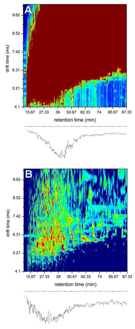
Part A shows a two-dimensional, t_R(t_D) plot of the raw data (A) for a single SCX fraction (sample 3). The plot is obtained by summing all TOF bins at each t_R and t_D value. Intensities are represented as a color map with the most intense level set at 150 counts. The representation indicates that individual two-dimensional bins are saturated across a wide range of retention and drift times. Part B shows the same data when plotted as a two-dimensional, t_R(t_D) base-peak diagram. This plot is obtained by extracting the intensity value obtained for the most intense m/z value in the MS measurement (extracted for every t_R (t_D) position to create the contour plot). The traces below each contour plot show the ion chromatograms obtained by integrating all t_D bins at each t_R for the respective 2D plots. For more details about the generation of these datasets see text references and discussion therein.

A feeling about the resolution and peak capacity associated with these dimensions of separation can be obtained from a two-dimensional t_R(t_D) base-peak plot (Figure 2B) derived from a single LC-IMS-MS analysis. This plot shows only the most intense peaks across all flight times. A significant advantage of this type of plot is that it provides a feeling for the importance of including an ion mobility dimension. Many different ions have identical retention times. From the widths of peaks in each dimension, and the range over which they are observed, we estimate the experimental two-dimensional LC-IMS peak capacity to be ~6000–9000.

Figure 2 also shows a plot of the intensities and positions of peaks as they are projected onto only the LC axis. This provides an additional feeling about the relationship of sample complexity to experimental peak capacity. In this case essentially all features that are observable in the LC dimension are comprised of many peaks

Reproducibility of identified peptide positions

It is important to assess the reproducibility of peaks. Analysis of data for assignments obtained from sequential triplicate runs of a single sample shows that peptide ion peak positions within the multidimensional are highly reproducible. Along the t_R and t_D dimensions, the percent relative uncertainty in position (from three analyses) is 1% and 2%, respectively. A similar comparison of the same peaks for three different samples yields a reproducibility of 4.8% and 2% for these respective dimensions. Note that the position of a peak in the drift time dimension does not vary for different samples.

Accumulation of the plasma proteome map

Peaks associated with peptide ions from the SCX-LC-IMS-MS datasets are identified by combining information from the precursor MS spectra with the CID-MS spectra. Figure 3 shows examples of three typical CID-MS spectra (at specific values of t_SCX, t_R, and t_D, for fragment ions; precursor data not shown). Upon analysis the overall assignments are consistent with peaks that correspond to primarily y-type and b-type ions for three peptide sequences (VSFLSALEEYTK, DSVTGTLPK, and VEVVDEER) that are unique to three different proteins (apolipoprotein A-I, kallikrein and troponin I, respectively). These data and assignments are typical of most of the features that are assigned in our datasets. We have focused on these three assignments because they allow some insight about the dynamic range associated with the raw data as well as the experiment. The plots have been normalized and so, as indicated in the figure, the peaks assigned to apolipoprotein are a factor of 400 times more intense than those for troponin I. This is consistent with the large difference in concentrations expected for these proteins (~mg mL⁻¹ to ng mL⁻¹ for these respective proteins⁹²). The concentration of kallikrein is reported to be in the ~40 μg mL^−1.80 From this, we see that generally the intensities of assigned features are qualitatively ordered in a fashion that reflects the concentrations of proteins (in cases where such data exists). However, there is a large mismatch associated with the range of measured intensities compared with the range of known concentrations. This may reflect the fact that some low abundance components are falsely assigned as we dig into the low-intensity features of our datasets for database searches. An alternative explanation is that variations in physical properties (e.g., ionization efficiency, solubility, and dissociation behavior), or unexpected differences in concentration of some specific peptides from low abundance proteins (due to biological accumulation or loss), limit the accuracy of quantitative comparisons.

Figure 3.

The plots on the right show fragmentation spectra of three identified peptides that have been identified based on database assignments (see text). These spectra are generated experimentally when the second field region of the split-field drift tube is modulated to high-field conditions sufficient to induce fragmentation. The low-field modulation data associated with measurement of the precursor ions (acquired in alternating fashion throughout the entire dataset) is not shown. The spectra that are shown are consistent with the VSFLASALEEYTK, DSVTGTLPK, and VEVVDEER sequences that are unique to the proteins apolipoprotein A-I, plasma kallikrein, and troponin I. The labels given to fragment ions in the spectra are generated by the database assignment and show a preponderance of y-type fragments (generally the observation for fragments generated at high-fields in these studies). The sequences to the left correspond to the total amino acid sequences of each of the respective proteins and those regions that are covered by assignments of peptides based on this approach are shown in red. Also indicated is number of unique peptide ions identified for each protein and the percentage of the sequence that has been identified by the analysis. See text for details.

Analysis of all datasets leads to 57192 ion assignments (hits). Of these, 37842 correspond to unique peptide sequences. Assuming that these sequences arise from a protein that existed in plasma this list leads to 9087 unique protein assignments. Many of the catalogued proteins have multiple peptide hits. Figure 3 provides an example of how the number of peptide hits may vary over the list of proteins. For the apolipoprotein A-I sequence analysis of all datasets leads to 930 hits of 39 different peptides. This corresponds to ~88% of the total sequence of the protein. Only six short peptides and one longer peptide were not included in the coverage: MK, AK, AR, QR, LAAR, LNTQ, and AAVLTLAVLFLTGSQAR. Interestingly MK, AK, AR, and QR are not unique and thus although we have detected these peptides it is not known whether or not they arise from apolipoprotein A-I. The LNTQ sequence is not a tryptic sequence and therefore was not included in our search algorithm. Additionally, none of these peptides (with the exception of the 17-residue peptide) would meet one of our search criteria (imposed after database assignment and used to reduce the number of false positives –that fragment ions must correspond to cleavage between at least five residues). The kallikrein and troponin I assignments are based on six and two hits, respectively. In these cases we find no evidence for large regions of the sequence. Because of this, assignments are far less robust (as discussed below).

Tables 1 and 2 provide a means of illustrating the structure of the overall map. Note that the tables that are shown are for example only. The complete maps are provided as supplementary information in Tables SI and SII, respectively. Table 1 is an accumulation of all uniquely assigned peptides and their corresponding proteins. It includes the positions (in all dimensions of the analysis) and intensities of peaks, the homology scores used to make each assignment, the corresponding protein and its accession number. In total Table SI contains entries for 37842 unique peptide ions. A useful way of understanding the information in Table SI comes from the representation of their LC, IMS and MS positions as shown in Figure 4. This plot shows the positions of the 100000 most intense features that appear from the triplicate analysis of sample 1. Features associated with all eight of the SCX fractions are included. The arrows represent features that are associated with specific assignments for four proteins (the three described in Figure 3 as well as transthyretin). In this case there are many more positions associated with the detection of apolipoprotein A-I than with detection of troponin. Although we have not analyzed the data in this fashion, knowledge of the positions of peaks will further corroborate assignments of the other datasets. In addition, the accumulation of data in Table SI provides valuable information for future work that would aim to predict SCX-, LC-retention times and mobilities based on sequences and charge states.

Table 1.

Peptide assignments from the integrated analysis of the human plasma samples.^a

Acc. # b	Protein Nameb	Peptide Sequencec	zd	tSCX{tR[tD(m/z)]}e	Intensityf	Scoreg
P02647	Apolipoprotein A-I precursor (Apo-AI) (ApoA-I)	DYVSQFEGSALGK	2	2.2 {44.04 [6.79 (701.38)]}	1.07E+05	93
		VSFLSALEEYTKK	3	5.2 {54.26 [5.58 (505.84)]}	1.22E+05	91
		LLDNWDSVTSTFSK	2	3 {49.43 [7.2 (807.34)]}	1.72E+04	89
		VSFLSALEEYTK	2	4.9 {63.28 [7.03 (694.15)]}	4.52E+05	87
		VSFLSALEEYTKK	2	6 {52.71 [5.69 (758.44)]}	3.50E+03	86
P01024	Complement C3 precursor [Contains: C3a anaphylatoxin]	RIPIEDGSGEVVLSR	3	4.7 {33.07 [5.79 (543.35)]}	1.52E+05	116
		SNLDEDIIAEENIVSR	2	2.8 {40.26 [7.19 (909.18)]}	3.69E+03	106
		VPVAVQGEDTVQSLTQGDGVAK	3	2 {39.16 [6.89 (733.77)]}	2.16E+04	103
		ENEGFTVTAEGK	2	3.3 {24.18 [6.58 (641.47)]}	5.95E+04	98
		SEETKENEGFTVTAEGK	3	4.5 {29.01 [6.17 (619.76)]}	1.61E+05	96
P02774	Vitamin D-binding protein precursor (DBP) (Group-specific component) (Gc-globulin) (VDB)	VPTADLEDVLPLAEDITNILSK	3	3.7 {92.25 [7.12 (789.88)]}	2.02E+05	112
		LAQKVPTADLEDVLPLAEDITNILSK	3	4.1 {85.13 [7.76 (936.6)]}	7.59E+04	108
		HQPQEFPTYVEPTNDEICEAFR	3	7.5 {38.48 [6.87 (903.29)]}	9.51E+03	105
		KFPSGTFEQVSQLVK	3	5.2 {40.65 [5.86 (565.81)]}	8.15E+04	90
		SCESNSPFPVHPGTAECCTK	3	3.9 {23.45 [6.48 (755.97)]}	2.41E+04	79

^aFor a complete list of the 38505 unique peptide ions, see Table S1 in the supplementary information.

^bProtein accessison numbers and names have been obtained from the Swiss-Prot noneredundant human protein database (http://ca.expasy.org/)

^cMost frequently observed peptides for indicated proteins

^dCharge states obeserved for indicated peptides yielding the highest Mascot ion scores

^eAverage nested multidimensional retention and drift times as well as m/z values for indicated peptides [t_SCX(fraction number), t_R(min), t_D(ms), m/z].

^fSummed precursor ion intensities obtained for each peptide assigned across the dataset

^gHighest Mascot ion score obtained for the indicated peptide.

Table 2.

List of the twenty proteins with the greatest number of peptide hits.^a

	Acc. #b	Protein Nameb	ΣHitsc	1d	2	3	4	5	ΣIntensitye	1	2	3	4	5
1	P02647	Apolipoprotein A-I precursor	930	218	241	212	112	147	2169900	226637	464912	269388	637943	571020
2	P01024	Complement C3 precursor	928	342	152	209	113	112	1856387	333768	279329	269584	547142	426564
3	P01023	Alpha-2-macroglobulin precursor	686	235	84	149	116	102	1730600	247284	169271	239802	698342	375901
4	P02671	Fibrinogen alpha/alpha-E chain precursor	491	114	102	111	74	90	1054699	90674	165561	118192	424895	255377
5	P04114	Apolipoprotein B-100 precursor	454	226	43	106	29	50	721764	196098	70513	138835	75778	240540
6	P02675	Fibrinogen beta chain precursor	445	104	118	103	52	68	991485	100976	168098	132819	283699	305893
7	P01028	Complement C4 precursor	425	86	115	88	59	77	847398	77866	199007	123065	226630	220830
8	P02679	Fibrinogen gamma chain precursor	369	67	105	77	35	85	647453	57521	121342	95082	104062	269446
9	P02652	Apolipoprotein A-II precursor	331	60	60	93	64	54	1102974	45471	147711	129048	580378	200366
10	P02774	Vitamin D-binding protein precursor	274	81	78	58	26	31	601450	75345	138687	79062	142727	165629
11	P02790	Hemopexin precursor	242	87	47	50	13	45	641994	96719	101316	78435	72161	293363
12	P00450	Ceruloplasmin precursor	210	63	48	49	20	30	412353	92774	92812	69970	41018	115779
13	P08603	Complement factor H precursor	196	59	35	39	49	14	331465	52557	48127	58215	133929	38637
14	Q14624	Inter-alpha-trypsin inhibitor heavy chain H4 precursor	189	62	24	52	29	22	265317	42041	44009	65784	71135	42348
15	P00734	Prothrombin precursor	177	69	29	48	12	19	293207	63472	36126	65730	49657	78222
16	P01042	Kininogen precursor	165	43	44	31	28	19	306598	43192	72474	46571	78245	66116
17	P02749	Beta-2-glycoprotein I precursor	152	52	38	32	12	18	281490	50874	82110	38698	19100	90708
18	P00751	Complement factor B precursor	151	45	21	30	34	21	363982	48586	19614	30182	207127	58473
19	P02765	Alpha-2-HS-glycoprotein precursor	150	22	47	35	13	33	235437	20094	54310	40283	69528	51222
20	P02763	Alpha-1-acid glycoprotein 1 precursor	142	27	38	27	30	20	241833	24242	23594	27111	95228	71658
Totals			7107	2062	1469	1599	920	1057	15097786	1986191	2498923	2115856	4558724	3938092

^aFor a complete list of proteins identified from protein database searches see Table S2 in the supplementary information

^bProtein accession numbers and names have been obtained from the Swiss-Prot nonredundant human protein database (http://ca.expasy.org/sprot/)

^cTotal number of peptide ion determinations for each protein.

^dSample number. Each sample was analyzed in triplicate (see text for details).

^eSummed precursor ion intensity obtained from all of the peptide ion assignments.

Figure 4.

A three-dimensional dot plot representation of the positions of peaks (in the retention time, drift time, and m/z dimensions) that are obtained from the 1×10⁵ most intense features (orange) observed during the triplicate LC-IMS-MS analyses of all SCX fractions associated with sample 1. Superimposed on the plot are the positions for >10,000 features that have been assigned to peptides (blue). The arrows indicate some of the precursor ion positions of peptides identified for the four proteins labeled. This representation is intended to provide the reader with the impression that the possible existence of an abundant protein in plasma (such as apolipoprotein A-I) could be tested at many positions in the map and therefore upon comparison there should be little ambiguity regarding its detection; whereas, a low-abundance protein (such as troponin I) may be represented at only a single position leading to significant uncertainty about its detection. See text for discussion.

The example shown as Table 2 lists 20 proteins that are identified from assignments made on data for all five samples. Those chosen here correspond to the most robust assignments (in that they represent our top 20 in terms of cumulative hits). In addition to information about the number of hits, we also include the integrated ion intensities for the precursor ion peaks that were assigned.⁸¹ The number of peptide ion assignments (hits) and the summed intensities are highly correlated. For example, a comparison of the number of peptide hits and integrated intensities for the extremes listed in Table 2 shows that there is a factor of ~7 times (930/142) more hits, corresponding to ~9 times (2.2×10⁶/2.4×10⁵) more ion intensity for the first entry (apolipoprotein A-I) compared with the 20^th entry (alpha-1-acid glycoprotein 1 precursor). An additional impression about the number of times different proteins are identified based on this approach can be obtained by examining Figure 5. This analysis shows that 1362 proteins are assigned by at least 10 peptide hits. This number decays dramatically as the number of hits increases. For example, only 70 proteins are found to be defined by more than 40 peptide hits.

Figure 5.

Bar graph showing the total number of proteins as a function of observed peptide hits per protein. The numbers for all assigned proteins are given in the supplementary information (Table S2).

As a final comment we note that most of the peaks in these datasets do not lead to assignments (less than 0.1% of the precursor ion peaks are assigned using the present criteria). The low fraction of assignments may result from several factors: limitations in the quality of the CID data generated in the drift tube (a relatively new approach that has not been tested extensively); substantial overlap of fragments from multiple different precursor ions that complicates spectra; and, the restriction of assignments to only tryptic fragments containing up to only one missed cleavage and no considerations of post-translational modifications.

Considerations associated with detection of false positives

Figure 6 shows a representation of Table S2 in terms of the total number of hits that are obtained for each of the 9087 entries associated with at least one hit. An issue that arises is which assignments should be trusted as components that are likely to be detectable with this type of approach. Examination of these data show that there is an apparent transition in the curve that occurs at about 60 –essentially the number of proteins that are assigned using 2D gels,¹⁵ (comprised of mostly the high-abundance classical plasma proteins).³ Our expectation is that the total number of hits should be roughly proportional to the protein concentration (and size, larger proteins will have more peptides that can be detected). Thus, the transition at around 60 proteins reflects the fact that the concentrations of many proteins fall just slightly below the detection limits of the earlier technologies.

Figure 6.

The top graph shows the percentage of false positive assignments for each peptide hit level from the random peptide hit removal analysis (see text for description) using the 10% (red) and 30% (blue) false positive rate estimates. Note that the 30% limit is a factor of three times greater than the upper limit of the (6 to 10%) range established in the false-positive rate estimate and is included to provide a feeling about an extreme limit (see text for discuussion). The arrow shows the peptide hit threshold for which no proteins were randomly removed at 6 hits and above (at a 10% false positive rate) and less than 1 in 20 protein assignments is considered a false positive (from the 30% trace). The bottom graph shows a log-log plot of the total number of peptide hits for each identified protein (Table S1, supplementary information). The dashed line shows the peptide hit level for the 100^th protein (35 hits). The 6-hit threshold (obtained from the top plot) is also shown with an arrow which indicates the cutoff between the 2928 proteins that are defined as high-confidence assignments (to the left of the threshold) and the 6159 low-confidence assignments (to the right of the threshold). An additional arrow at protein number 60 indicates the number of proteins that were detected using 2D gel techniques, most of which are classical plasma proteins (see text). The change in slope near this value reflects a transition in concentrations between these more abundant components (mostly classical plasma proteins) and those that arise from tissue leakage.

Beyond this number the issue of how many proteins are detectable in plasma requires that we understand the threshold for detection in more detail. Probability-based scoring algorithms are prone to making false assignments,⁴⁰ even with the additional assignment criteria that we described above. Because of this it is worthwhile to examine the false-positive rate in more detail. This is done by determining the rate of assignments that are made when a nonsensical protein database is used.^40,82–85 This database was created by inverting all protein sequences in the Swiss-Prot non-redundant human database. Estimated false-positive rates range from ~6 to 10% from replicate analyses.⁹

Figure 6 shows a plot of the number of times that a protein would be randomly assigned [using a 10% false-positive rate (the upper end of the range) and three times this value (30%)]. From this analysis we observe that a substantial fraction of those proteins that are assigned based on only a few hits are likely to be random assignments.⁸⁶ For example, 45 to 88% of assignments based on a single peptide hit are random (using the 10% and 30% false-positive rate limits, respectively). This number drops to 12 to 64% of the assignments if two hits are used. A random assignment rate of fewer than one in 20 is found at the 30% false positive rate when at least six hits are used to identify a single protein (note that no false-positives are predicted at six hits when our 10% false positive rate is used). From the threshold value of 6 we determine that 2928 of these identifications are high-confidence assignments. We anticipate that more low-abundance species will become high-confidence assignments as more experiments are conducted.

As a final note, in a preliminary set of experiments using a substantially longer drift tube (~3 m) that is operated under conditions that provide a factor of ~3 to 4 times improvement in peak capacity (in the drift time dimension)⁹ we find substantial increases in the MASCOT scores for peptides associated with abundant proteins (in direct comparisons of the same sample analyzed on different instruments. This result is consistent with the idea that simultaneous elution of multiple components interferes with assigning features. At this stage, comparisons can only be made for abundant species that are already known to be present in plasma. We are currently in the process of improving the sensitivity of this instrument so that this method can also be used to confirm (or dispute) the assignments we have made for lower abundance components.

Features of the plasma proteome map

It is instructive to consider the types of proteins observed in the high-confidence list. Anderson, Smith and their collaborators have previously assessed the content of plasma based on considerations of Gene Ontology (GO).^15,21,39 In general terms, this provides a representation of where in the cell different proteins are found. Figure 7 shows the percentage of each GO component in the entire Swiss-Prot database as well as the percentage of each component in the current plasma map. The percentages are significantly different for several key components (e.g., the extracellular, cytoplasmic, and nuclear components). The differences further corroborate the notion that the map is not composed of random assignments. If it were, the percentages of each GO component in the plasma map would more closely mimic those in the protein database. Perhaps a better comparison is to look at the protein makeup by including a weighting factor for each protein based on the number of peptide ion hits. Figure 7C shows the change in GO component percentages when the protein list is weighted by the number of peptide hits used to represent it. A noticeable increase in the percentage (13 to 28%) of the extracellular component is observed with a decrease in the overall percentage (39 to 28%) of the membrane component. This is consistent with the greater number of observations of classical plasma proteins.

Figure 7.

Major gene ontology (GO) component percentages for the entire human proteome (A), the plasma proteome generated from IMS-MS experiments (B), as well as the proteome map weighted by the number of protein hits (C). See text for discussion.

Comparison of this map with others

As a check of consistency, it is useful to compare the high-confidence list of proteins with other maps of plasma. We arbitrarily began by comparing 26 proteins that we observed with at least 100 hits to our previous SCX-LC-IMS-MS analysis in Table 3.⁹ Although there is substantial variability about the number of peptide hits, most (22) of the 26 proteins are detected in the previous study. A comparison to our complete list observed previously shows that, 252 of the 438 proteins reported previously are reported as high-confidence assignments in the current studies. The overlap can be found in the supplementary information (Table S3).

Table 3.

List of top 26 proteins identified with more than 100 hits in the current analysis and the overlap with the previous SCX-LC-IMS-MS, the 1175 nonredundant, and the HUPO core datasets.^a

	Acc. #b	Protein Nameb	ΣHitsc	1d	2	3	4	5	SCX-LC-IMS-Mse	1175 NRf	HUPOg
1	P02647	Apolipoprotein A-I precursor (Apo-	930	218	241	212	112	147	18	6	78
2	P01024	Complement C3 precursor [Contai	928	342	152	209	113	112	17	4	246
3	P01023	Alpha-2-macroglobulin precursor (	686	235	84	149	116	102	16	5	207
4	P02671	Fibrinogen alpha/alpha-E chain pre	491	114	102	111	74	90	9	3	65
5	P04114	Apolipoprotein B-100 precursor (Ap	454	226	43	106	29	50	10	4	317
6	P02675	Fibrinogen beta chain precursor [C	445	104	118	103	52	68	7	3	51
7	P01028	Complement C4 precursor [Contai	425	86	115	88	59	77	12	5	155
8	P02679	Fibrinogen gamma chain precursor	369	67	105	77	35	85	10	1	50
9	P02652	Apolipoprotein A-II precursor (Apo-	331	60	60	93	64	54	0	4	17
10	P02774	Vitamin D-binding protein precurso	274	81	78	58	26	31	5	5	47
11	P02790	Hemopexin precursor (Beta-1B-gly	242	87	47	50	13	45	4	3	86
12	P00450	Ceruloplasmin precursor (EC 1.16.	210	63	48	49	20	30	2	4	131
13	P08603	Complement factor H precursor (H	196	59	35	39	49	14	1	4	125
14	Q14624	Inter-alpha-trypsin inhibitor heavy c	189	62	24	52	29	22	2	5	86
15	P00734	Prothrombin precursor (EC 3.4.21.	177	69	29	48	12	19	6	5	69
16	P01042	Kininogen precursor (Alpha-2-thiol	165	43	44	31	28	19	1	8	52
17	P02749	Beta-2-glycoprotein I precursor (Ap	152	52	38	32	12	18	3	4	73
18	P00751	Complement factor B precursor (E	151	45	21	30	34	21	2	4	76
19	P02765	Alpha-2-HS-glycoprotein precursor	150	22	47	35	13	33	2	4	65
20	P02763	Alpha-1-acid glycoprotein 1 precurs	142	27	38	27	30	20	3	3	45
21	P06727	Apolipoprotein A-IV precursor (Apo	130	45	39	22	11	13	3	5	45
22	P04217	Alpha-1B-glycoprotein precursor (A	121	35	21	19	20	26	0	3	43
23	P01008	Antithrombin-III precursor (ATIII) (P	120	61	12	32	6	9	3	4	67
24	P01011	Alpha-1-antichymotrypsin precurso	117	54	16	23	9	15	0	4	76
25	P19827	Inter-alpha-trypsin inhibitor heavy c	117	29	32	16	23	17	1	5	56
26	P10909	Clusterin precursor (Complement-a	106	38	17	28	13	10	0	4	53
Totals			7818	2324	1606	1739	1002	1147	137	109	2381

^aFor a complete list of proteins that overlap with the previous IMS, 1175 nonredundant, and HUPO datasets, see Tables S3, S4, and S5 in the supplementary information.

^bAccession numbers and names have been obtained from the Swiss-Prot human protein database. (http://ca.expasy.org/sprot/)

^cTotal number of peptide ion determinations for each protein.

^dSample number. Each sample was analyzed in triplicate. [See text for details.]

^eNumber of peptides hits from the previous SCX-LC-IMS-MS analysis of human plasma. See reference 9 for details.

^fNumber of peptide hits from the 1175 nonredundant protein list compiled by Anderson and coworkers. See reference 15 for details.

^gNumber of distinct peptides listed for the high confidence HUPO dataset that includes 3020 total proteins. See reference ²⁵ for details.

A second comparison that can be made involves the 1175 non-redundant dataset compiled by Anderson and coworkers.¹⁵ Again, our top 26 proteins all overlap with the Anderson list (Table 3). Remember that from their analysis it was determined that only 46 proteins were observed from all sources. Here we note that all 46 of those proteins are observed as high-confidence assignments in the present study. Interestingly they are all found in our top 100 proteins. A more detailed comparison of the 2928 high-confidence protein assignments with the 1175 protein list shows that 321 proteins are found in both (see Table S4).

Finally, we have compared some of our map to some data reported by the plasma proteome project (PPP). In the case of the 26 proteins in Table 3, all are also reported in the PPP dataset. It is more difficult to compare to the complete PPP database because the system of protein accession numbers is from multiple independently curated databases. Comparison by name and accession number (a by hand comparison) of our top 300 proteins with the 3020 core dataset provided by HUPO shows that 185 are found in both datasets (provided as Table S5 in the supplementary information).

Considerations of dynamic range

Commercial MS instruments have a dynamic range of ~10²–10^5.87–91 The inclusion of an IMS dimension is expected to improve this due to the removal of chemical noise.⁸ From assignments that fall at the threshold associated with high-confidence assignments we can assess the expected dynamic range of this system. As examples, troponin I, prostatic acid phosphatase, and thyroxine-binding globulin protein each were observed with 5 peptide hits (just below the high-confidence threshold). The concentrations of these proteins are 1.0, 1.7, and 14.1 ng-mL⁻¹, respectively.⁹² The proteins thyroglobulin, tissue-type plasminogen activator, and plasma kallikrein are observed 21, 8, and 9 times, respectively, in the plasma map. These proteins have nominal plasma concentrations of 19.0, 5.5, and 55.0 ng-mL⁻¹, respectively. This analysis suggests that for most species we might expect an estimated lower limit for identification in the low ng-mL⁻¹ range; this would suggest an experimental dynamic range of 10⁵–10⁶.

Within the high-confidence dataset, a single interleukin (reported as IL-16 precursor in Table S1, but only represented with hits in the body of the protein) was observed (15 peptide ion hits across seven unique regions of sequence). Based on our confidence analysis we expect this to be a reproducible signal with this approach. However, clearly some additional caution should be taken in considering this assignment (as with any other assignment for a protein that is known to exist in extremely low abundances). Assuming an IL-16 protein concentration of ~10 pg-mL⁻¹ (within plasma, and no sample loss during workup), would require detection of ~5 pg or ~75 attomols. This approaches the ultimate measured detection limit for this instrumentation.⁵⁴ We include the result in our high-confidence list because it meets the imposed criteria. However, we urge the users of this map to approach this and other assignments for species that are known to exist at very low abundances cautiously.

Summary and conclusions

A multidimensional SCX-LC-IMS-MS experiment combined with a database assignment approach has been used to generate a plasma proteome map. Triplicate analysis of plasma from five healthy people results in assignment of 9087 proteins of which 2928 are expected to be reproducibly detected with this experimental approach. The map contains information about protein accession numbers and names, peptides used for assignment as well as peak position within the multidimensional space and intensities. Comparison of these assignments with those found in other maps suggests good agreement for the most abundant components. There is reasonable agreement about the first several hundred proteins in our map with other datasets. Beyond this level, many components in the map developed here appear to be unique to our approach; additionally, this analysis does not assign many features that are included in other summaries.

References

- 1.Wasinger VC, Cordwell SJ, Cerpa-Poljak A, Yan JX, Gooley AA, Wilkins MR, Duncan MW, Harris R, Williams KL, Humphery-Smith I. Progress with Gene-Product Mapping of the Mollicutes: Mycoplasma Genitalium. Electrophoresis. 1995;16:1090–1094. doi: 10.1002/elps.11501601185. [DOI] [PubMed] [Google Scholar]
- 2.For proteomic platform technology development information see the following reviews andreferences therein: Hancock WS, Apffel AJ, Chakel JA, Hahnenberger KC, Choudhary G, Traina J, Pungor E. Integrated Genomic/Proteomic Analysis. Anal Chem. 1999;71:742A–748A. doi: 10.1021/ac9907641.Schweitzer B, Kingsmore SF. Measuring Proteins on Microarrays. Curr Opin Biotech. 2002;13:14–19. doi: 10.1016/s0958-1669(02)00278-1.Figeys D. Proteomics in 2002: a Year of Technical Development and Wide-Ranging Applications. Anal Chem. 2003;75:2891–2905. doi: 10.1021/ac030142m.Romijn EP, Krijgsveld J, Heck AJR. Recent Liquid Chromatographic-(Tandem) Mass Spectrometric Applications in Proteomics. J Chromat A. 2003;1000:589–608. doi: 10.1016/s0021-9673(03)00178-x.Aebersold R, Mann M. Mass Spectrometry-Based Proteomics. Nature. 2003;422:198–207. doi: 10.1038/nature01511.Page JS, Masselon CD, Smith RD. FTICR Mass Spectrometry for Qualitative and Quantitative Bioanalyses. Curr Opin Biotech. 2004;15:3–11. doi: 10.1016/j.copbio.2004.01.002.Anderson L. Candidate-Based Proteomics in the Search for Biomarkers of Cardiovascular Disease. J Physiol-London. 2005;563:23–60. doi: 10.1113/jphysiol.2004.080473.
- 3.Anderson NL, Anderson NG. The Human Plasma Proteome: History, Character, and Diagnostic Prospects. Mol Cel Proteomics. 2002;1:845–867. doi: 10.1074/mcp.r200007-mcp200. [DOI] [PubMed] [Google Scholar]
- 4.Liu X, Plasencia M, Ragg S, Valentine SJ, Clemmer DE. Development of High-Throughput Dispersive LC-Ion Mobility-TOFMS Techniques for Analyzing the Human Plasma Proteome. Brief Funct Genomics Proteomics. 2004;3:177–186. doi: 10.1093/bfgp/3.2.177. [DOI] [PubMed] [Google Scholar]
- 5.The latest version of the Swiss-Prot protein database can be found at the following web address: http://www.expasy.uniprot.org/database/knowledgebase.shtml.
- 6.Tirumalai RS, Chan KC, Prieto DA, Issaq HJ, Conrads TP, Veenstra TD. Characterization of the Low Molecular Weight Human Serum Proteome. Mol Cel Proteomics. 2003;2:1096–1103. doi: 10.1074/mcp.M300031-MCP200. [DOI] [PubMed] [Google Scholar]
- 7.Putnam FW, editor. The Plasma Proteins: Structure, Function and Genetic Control. Academic Press; New York: 1975. [Google Scholar]
- 8.Counterman AE, Hilderbrand AE, Srebalus Barnes CA, Clemmer DE. Formation of Peptide Aggregates during ESI: Size, Charge, Composition, and Contributions to Noise. J Am Soc Mass Spectrom. 2001;12:1020–1035. [Google Scholar]
- 9.Valentine SJ, Plasencia MD, Liu X, Krishnan M, Naylor S, Udseth HR, Smith RD, Clemmer DE. Toward Plasma Proteome Profiling with Ion Mobility-Mass Spectrometry. J Proteome Res. 2006;5:2977–2984. doi: 10.1021/pr060232i. [DOI] [PubMed] [Google Scholar]
- 10.Anderson NL, Anderson NG. A Two-Dimensional Gel Database of Human Plasma Proteins. Electrophoresis. 1991;12:883–906. doi: 10.1002/elps.1150121108. [DOI] [PubMed] [Google Scholar]
- 11.Ueno I, Sakai T, Yamaoka M, Yoshida R, Tsugita A. Analysis of Blood Plasma Proteins in Patients with Alzheimer’s Disease by Two-Dimensional Electrophoresis, Sequence Homology and Immunodetection. Electrophoresis. 2000;21:1832–1845. doi: 10.1002/(SICI)1522-2683(20000501)21:9<1832::AID-ELPS1832>3.0.CO;2-7. [DOI] [PubMed] [Google Scholar]
- 12.Pieper R, Gatlin CL, Makusky AJ, Russo PS, Schatz CR, Miller SS, Su Q, McGrath AM, Estock MA, Parmar PP, Zhao M, Huang ST, Zhou J, Wang F, Esquer-Blasco R, Anderson NL, Taylor J, Steiner S. The Human Serum Proteome: Display of Nearly 3700 Chromatographically Separated Protein Spots on Two-Dimensional Electrophoresis Gels and Identification of 325 Distinct Proteins. Proteomics. 2003;3:1345–1364. doi: 10.1002/pmic.200300449. [DOI] [PubMed] [Google Scholar]
- 13.Anderson L, Anderson NG. High Resolution Two-Dimensional Electrophoresis of Human Plasma Proteins. Proc Natl Acad Sci USA. 1977;74:5421–5425. doi: 10.1073/pnas.74.12.5421. [DOI] [PMC free article] [PubMed] [Google Scholar]
- 14.For a discussion of early 2DE work see: Dunn MJ. Two-Dimensional Gel Electrophoresis of Proteins. J Chromatogr. 1987;418:145–185. doi: 10.1016/0378-4347(87)80008-7.and references therein
- 15.Anderson NL, Polanski M, Pieper R, Gatlin T, Tirumalai RS, Conrads TP, Veenstra TD, Adkins JN, Pounds JG, Fagan R, Lobley A. The Human Plasma Proteome: a Nonredundant List Developed by Combination of Four Separate Sources. Mol Cell Proteomics. 2004;3:311–326. doi: 10.1074/mcp.M300127-MCP200. [DOI] [PubMed] [Google Scholar]
- 16.Wolters DA, Washburn MP, Yates JR. An Automated Multidimensional Protein Identification Technology for Shotgun Proteomics. Anal Chem. 2001;73:5683–5690. doi: 10.1021/ac010617e. [DOI] [PubMed] [Google Scholar]
- 17.Washburn MP, Wolters D, Yates JR. Large-Scale Analysis of the Yeast Proteome by Multidimensional Protein Identification Technology. Nat Biotechnol. 2001;19:242–247. doi: 10.1038/85686. [DOI] [PubMed] [Google Scholar]
- 18.Peng J, Elias JE, Thoreen CC, Licklider LJ, Gygi SP. Evaluation of Multidimensional Chromatography Coupled with Tandem Mass Spectrometry (LC/LC-MS/MS) for Large-Scale Protein Analysis: the Yeast Proteome. J Proteome Res. 2003;2:43–50. doi: 10.1021/pr025556v. [DOI] [PubMed] [Google Scholar]
- 19.Adkins JN, Varnum SM, Auberry KJ, Moore RJ, Angell NH, Smith RD, Springer DL, Pounds JG. Toward a Human Blood Serum Proteome: Analysis by Multidimensional Separation Coupled with Mass Spectrometry. Mol Cell Proteomics. 2002;1:947–955. doi: 10.1074/mcp.m200066-mcp200. [DOI] [PubMed] [Google Scholar]
- 20.Wu SL, Choudhary G, Ramstrom M, Bergquist J, Hancock WS. Evaluation of Shotgun Sequencing for Proteomic Analysis of Human Plasma Using HPLC Coupled with either Ion Trap or Fourier Transform Mass Spectrometry. J Proteome Res. 2003;2:383–393. doi: 10.1021/pr034015i. [DOI] [PubMed] [Google Scholar]
- 21.Shen Y, Jacobs JM, Camp DG, II, Fang R, Moore RJ, Smith RD, Xiao W, Davis RW, Tompkins RG. Ultra-High-Efficiency Strong Cation Exchange LC/RPLC/MS/MS for High Dynamic Range Characterization of the Human Plasma Proteome. Anal Chem. 2004;76:1134–1144. doi: 10.1021/ac034869m. [DOI] [PubMed] [Google Scholar]
- 22.Zhou M, Lucas DA, Chan KC, Issaq HJ, Petricoin EF, Liotta LA, Veenstra TD, Conrads TR. An Investigation into the Human Serum “Interactome”. Electrophoresis. 2004;25:1289–1298. doi: 10.1002/elps.200405866. [DOI] [PubMed] [Google Scholar]
- 23.Rose K, Bougueleret L, Baussant T, Böhm G, Botti P, Colinge J, Cusin I, Gaertner H, Gleizes A, Heller M, Jimenez S, Johnson A, Kussmann M, Menin L, Menzel C, Ranno F, Rodriguez-Tomé P, Rogers J, Saudrais C, Villain M, Wetmore D, Bairoch A, Hochstrasser D. Industrial-Scale Proteomics: From Liters of Plasma to Chemically Synthesized Proteins. Proteomics. 2004;4:2125–2150. doi: 10.1002/pmic.200300718. [DOI] [PubMed] [Google Scholar]
- 24.For results from the Plasma Proteome Project (PPP) collaboration sponsored by the Human Proteome Organization (HUPO), see the recent issue (13 in 2005) in the journal Proteomics. The entire issue describes the significant results obtained from the efforts of the collaborating laboratories.
- 25.Omenn GS, States DJ, Adamski M, Blackwell TW, Menon R, Hermjakob H, Apweiler R, Haab BB, Simpson RJ, Eddes JS, Kapp EA, Moritz RL, Chan DW, Rai AJ, Admon A, Aebersold R, Eng J, Hancock WS, Hefta SA, Meyer H, Paik Y, Yoo J, Ping P, Pounds J, Adkins J, Qian X, Wang R, Wasinger V, Wu CY, Zhao X, Zeng R, Archakov A, Tsugita A, Beer I, Pandey A, Pisano M, Andrews P, Tammen H, Speicher DW, Hanash SM. Overview of the HUPO Plasma Proteome Project: Results from the Pilot Phase with 35 Collaborating Laboratories and Multiple Analytical Groups, Generating a Core Dataset of 3020 Proteins and a Publicly-Available Database. Proteomics. 2005;5:3226–3245. doi: 10.1002/pmic.200500358. [DOI] [PubMed] [Google Scholar]
- 26.Chan KC, Lucas DA, Hise D, Schaefer CF, Xiao Z, Janini George M, Buetow KH, Issaq HJ, Veenstra TD, Conrads TP. Analysis of the Human Serum Proteome. Clin Proteomics. 2004;1:101–226. [Google Scholar]
- 27.Jiang L, He L, Fountoulakis M. Comparison of Protein Precipitation Methods for Sample Preparation Prior to Proteomic Analysis. J Chromatogr A. 2004;1023:317–320. doi: 10.1016/j.chroma.2003.10.029. [DOI] [PubMed] [Google Scholar]
- 28.Hsieh SY, Chen RK, Pan YH, Lee HL. Systematical Evaluation of the Effects of Sample Collection Procedures on Low-Molecular-Weight Serum/Plasma Proteome Profiling. Proteomics. 2006;6:3189–3198. doi: 10.1002/pmic.200500535. [DOI] [PubMed] [Google Scholar]
- 29.Liu T, Qian WJ, Mottaz HM, Gritsenko MA, Norbeck AD, Moore RJ, Purvine SO, Camp DG, II, Smith RD. Evaluation of Multiprotein Immunoaffinity Subtraction for Plasma Proteomics and Candidate Biomarker Discovery Using Mass Spectrometry. Mol Cell Proteomics. 2006;5:2167–2174. doi: 10.1074/mcp.T600039-MCP200. [DOI] [PMC free article] [PubMed] [Google Scholar]
- 30.Banks RE, Stanley AJ, Cairns DA, Barrett JH, Clarke P, Thompson D, Selby PJ. Influences of Blood Sample Processing on Low-Molecular-Weight Proteome Identified by Surface-Enhanced Laser Desorption/Ionization Mass Spectrometry. Clin Chem. 2005;51:1637–1649. doi: 10.1373/clinchem.2005.051417. [DOI] [PubMed] [Google Scholar]
- 31.Stone E, Gillig KJ, Ruotolo B, Fuhrer K, Gonin M, Schultz A, Russell DH. Surface-Induced Dissociation on a MALDI-Ion Mobility-Orthogonal Time-of-Flight Mass Spectrometer: Sequencing Peptides from an “In-Solution” Protein Digest. Anal Chem. 2001;73:2233–2238. doi: 10.1021/ac001430a. [DOI] [PubMed] [Google Scholar]
- 32.Wysocki VH, Resing KA, Zhang QF, Cheng GL. Mass Spectrometry of Peptides and Proteins. Methods. 2005;35:211–222. doi: 10.1016/j.ymeth.2004.08.013. [DOI] [PubMed] [Google Scholar]
- 33.Mikesh LM, Ueberheide B, Chi A, Coon JJ, Syka JE, Shabanowitz J, Hunt DF. The Utility of ETD Mass Spectrometry in Proteomic Analysis. Biochim Biophys Acta. 2006;1764:1811–1822. doi: 10.1016/j.bbapap.2006.10.003. [DOI] [PMC free article] [PubMed] [Google Scholar]
- 34.Dodds ED, Hagerman PJ, Lebrilla CB. Fragmentation of Singly Protonated Peptides via a Combination of Infrared and Collisional Activation. Anal Chem. 2006;78:8506–8511. doi: 10.1021/ac0614442. [DOI] [PubMed] [Google Scholar]
- 35.Zubarev R. Protein Primary Structure Using Orthogonal Fragmentation Techniques in Fourier Transform Mass Spectrometry. Expert Rev Proteomics. 2006;3:251–261. doi: 10.1586/14789450.3.2.251. [DOI] [PubMed] [Google Scholar]
- 36.Bakhtiar R, Guan ZQ. Electron Capture Dissociation Mass Spectrometry in Characterization of Peptides and Proteins. Biotechnol Letters. 2006;28:1047–1059. doi: 10.1007/s10529-006-9065-z. [DOI] [PubMed] [Google Scholar]
- 37.Fernandez FM, Wysocki VH, Futrell JH, Laskin J. Protein Identification via Surface-Induced Dissociation in an FT-ICR Mass Spectrometer and a Patchwork Sequencing Approach. J Am Soc Mass Spectrom. 2006;17:700–709. doi: 10.1016/j.jasms.2006.01.012. [DOI] [PubMed] [Google Scholar]
- 38.Riter LS, Gooding KM, Hodge BD, Julian RK. Comparison of the Paul Ion Trap to the Linear Ion Trap for Use in Global Proteomics. Proteomics. 2006;6:1735–1740. doi: 10.1002/pmic.200500477. [DOI] [PubMed] [Google Scholar]
- 39.Jacobs JM, Adkins JN, Qian WJ, Shen Y, Camp DG, II, Smith RD. Utilizing Human Blood Plasma for Proteomic Biomarker Discovery. J Proteome Res. 2005;4:1073–1085. doi: 10.1021/pr0500657. [DOI] [PubMed] [Google Scholar]
- 40.Cargile BJ, Bundy JL, Stephenson JL., Jr Potential for False Positive Identifications from Large Databases through Tandem Mass Spectrometry. J Proteome Res. 2004;3:1082–1085. doi: 10.1021/pr049946o. [DOI] [PubMed] [Google Scholar]
- 41.Kapp EA, Schutz F, Connolly LM, Chakel JA, Meza JE, Miller CA, Fenyo D, Eng JK, Adkins JN, Omenn GS, Simpson RJ. An Evaluation, Comparison, and Accurate Benchmarking of Several Publicly Available MS/MS Search Algorithms: Sensitivity and Specificity Analysis. Proteomics. 2005;5:3475–3490. doi: 10.1002/pmic.200500126. [DOI] [PubMed] [Google Scholar]
- 42.States DJ, Omenn GS, Blackwell TW, Fermin D, Eng J, Speicher DW, Hanash SM. Challenges in Deriving High-Confidence Protein Identifications from Data Gathered by a HUPO Plasma Proteome Collaborative Study. Nat Biotechnol. 2006;24:333–338. doi: 10.1038/nbt1183. [DOI] [PubMed] [Google Scholar]
- 43.St Louis RH, Hill HH. Ion Mobility Spectrometry in Analytical Chemistry. CRC Crit Rev Anal Chem. 1990;21:321–355. doi: 10.1021/ac00222a001. [DOI] [PubMed] [Google Scholar]
- 44.Clemmer DE, Hudgins RR, Jarrold MF. Naked Protein Conformations: Cytochrome c in the Gas Phase. J Am Chem Soc. 1995;117:10141–10142. [Google Scholar]
- 45.von Helden G, Wyttenbach T, Bowers MT. Conformation of Macromolecules in the Gas Phase: Use of Matrix-Assisted Laser Desorption Methods in Ion Chromatography. Science. 1995;267:1483–1485. doi: 10.1126/science.267.5203.1483. [DOI] [PubMed] [Google Scholar]
- 46.Chen YH, Hill HH, Wittmer DP. Thermal Effects on Electrospray Ionization Ion Mobility Spectrometry. Int J Mass Spectrom Ion Proc. 1996;154:1–13. [Google Scholar]
- 47.Gillig KJ, Ruotolo B, Stone EG, Russell DH, Fuhrer K, Gonin M, Schultz AJ. Coupling High-Pressure MALDI with Ion Mobility/Orthogonal Time-of-Flight Mass Spectrometry. Anal Chem. 2000;72:3965–3971. doi: 10.1021/ac0005619. [DOI] [PubMed] [Google Scholar]
- 48.Steiner WE, Clowers BH, English WA, Hill HH., Jr Atmospheric Pressure Matrix-Assisted Laser Desorption/Ionization with Analysis by Ion Mobility Time-of-Flight Mass Spectrometry. Rapid Commun Mass Spectrom. 2004;18:882–888. doi: 10.1002/rcm.1419. [DOI] [PubMed] [Google Scholar]
- 49.Myung S, Wiseman JM, Valentine SJ, Zoltán T, Cooks RG, Clemmer DE. Coupling Desorption Electrospray Ionization (DESI) with Ion Mobility/Mass Spectrometry for Analysis of Protein Structure: Evidence for Desorption of Folded and Denatured States. J Phys Chem B. 2006;110:5045–5051. doi: 10.1021/jp052663e. [DOI] [PubMed] [Google Scholar]
- 50.Shaffer SA, Prior DC, Anderson GA, Udseth HR, Smith RD. An Ion Funnel Interface for Improved Ion Focusing and Sensitivity Using Electrospray Ionization Mass Spectrometry. Anal Chem. 1998;70:4111–4119. doi: 10.1021/ac9802170. [DOI] [PubMed] [Google Scholar]
- 51.Kim T, Tolmachev AV, Harkewicz R, Prior DC, Anderson G, Udseth HR, Smith RD, Bailey TH, Rakov S, Futrell JH. Design and Implementation of a New Electrodynamic Ion Funnel. Anal Chem. 2000;72:2247–2255. doi: 10.1021/ac991412x. [DOI] [PubMed] [Google Scholar]
- 52.Lee YJ, Hoaglund-Hyzer CS, Taraszka JA, Zientara GA, Counterman AE, Clemmer DE. Collision-Induced Dissociation of Mobility-Separated Ions Using an Orifice-Skimmer Cone at the Back of a Drift Tube. Anal Chem. 2001;73:3549–3555. doi: 10.1021/ac010295e. [DOI] [PubMed] [Google Scholar]
- 53.Tang K, Shvartsburg AA, Lee H, Prior DC, Buschbach MA, Li F, Tomachev A, Anderson GA, Smith RD. High-Sensitivity Ion Mobility Spectrometry/Mass Spectrometry Using Electrodynamic Ion Funnel Interfaces. Anal Chem. 2005;77:3330–3339. doi: 10.1021/ac048315a. [DOI] [PMC free article] [PubMed] [Google Scholar]
- 54.Myung S, Lee YL, Moon MH, Taraszka JA, Sowell R, Koeniger SL, Hilderbrand AE, Valentine SJ, Cherbas L, Cherbas P, Kaufmann TC, Miller DF, Mechref Y, Novotny MV, Ewing M, Clemmer DE. Development of High-Sensitivity Ion Trap-IMS-TOF Techniques: A High-Throughput Nano-LC/IMS/TOF Separation of the Drosophila Fly Proteome. Anal Chem. 2003;75:5137–5145. doi: 10.1021/ac030107f. [DOI] [PubMed] [Google Scholar]
- 55.McLean JA, Russell DH. Sub-Femtomole Peptide Detection in Ion Mobility-Time-of-Flight Mass Spectrometry Measurements. J Proteome Res. 2003;2:427–430. doi: 10.1021/pr034004p. [DOI] [PubMed] [Google Scholar]
- 56.Dugourd P, Hudgins RR, Clemmer DE, Jarrold MF. High-Resolution Ion Mobility Measurements. Rev Sci Instrum. 1997;68:1122–1129. [Google Scholar]
- 57.Wu C, Siems WF, Asbury GR, Hill HH., Jr Electrospray Ionization High-Resolution Ion Mobility Spectrometry-Mass Spectrometry. Anal Chem. 1998;70:4929–4938. doi: 10.1021/ac980414z. [DOI] [PubMed] [Google Scholar]
- 58.Srebalus CA, Li J, Marshall WS, Clemmer DE. Gas-Phase Separations of Electrosprayed Peptide Libraries. Anal Chem. 1999;71:3918–3927. doi: 10.1021/ac9903757. [DOI] [PubMed] [Google Scholar]
- 59.Valentine SJ, Counterman AE, Hoaglund-Hyzer CS, Clemmer DE. Intrinsic Amino Acid Size Parameters from a Series of 113 Lysine-Terminated Tryptic Digest Peptide Ions. J Phys Chem B. 1999;103:1203–1207. [Google Scholar]
- 60.Shvartsburg AA, Siu KWM, Clemmer DE. Prediction of Peptide Ion Mobilities via a priori Calculations from Intrinsic Size Parameters of Amino Acid Residues. J Am Soc Mass Spectrom. 2001;12:885–888. doi: 10.1016/S1044-0305(01)00269-0. [DOI] [PubMed] [Google Scholar]
- 61.Valentine SJ, Counterman AE, Clemmer DE. A Database of 660 Peptide Ion Cross Sections: Use of Intrinsic Size Parameters for Bona Fide Predictions of Cross Sections. J Am Soc Mass Spectrom. 1999;10:1188–1211. doi: 10.1016/S1044-0305(99)00079-3. [DOI] [PubMed] [Google Scholar]
- 62.Mosier PD, Counterman AE, Jurs PC, Clemmer DE. Prediction of Peptide Ion Collision Cross Sections from Topological Molecular Structure and Amino Acid Parameters. Anal Chem. 2002;74:1360–1370. doi: 10.1021/ac0112059. [DOI] [PubMed] [Google Scholar]
- 63.Wyttenbach T, von Helden G, Batka JJ, Jr, Carlat D, Bowers MT. Effect of the Long-Range Potential on Ion Mobility Measurements. J Am Soc Mass Spectrom. 1997;8:275–282. [Google Scholar]
- 64.Shvartsburg AA, Jarrold MF. An Exact Hard-Sphere Scattering Model for the Mobilities of Polyatomic Ions. Chem Phys Lett. 1996;261:86–91. [Google Scholar]
- 65.Mesleh MF, Hunter JM, Shvartsburg AA, Schatz GC, Jarrold MF. Structural Information from Ion Mobility Measurements: Effects of the Long-Range Potential. J Phys Chem. 1996;100:16082–16086. [Google Scholar]
- 66.Clemmer DE, Jarrold MF. Ion Mobility Measurements and their Applications to Clusters and Biomolecules. J Mass Spectrom. 1997;32:577–592. [Google Scholar]
- 67.Hoaglund-Hyzer CS, Counterman AE, Clemmer DE. Anhydrous Protein Ions. Chem Rev. 1999;99:3037–3079. doi: 10.1021/cr980139g. [DOI] [PubMed] [Google Scholar]
- 68.Wyttenbach T, Bowers MT. Modern Mass Spectrom, Topics Curr Chem: Chemistry and Materials Science. Vol. 225. Springer; Berlin/Heidelberg: 2003. Gas-Phase Conformations: The Ion Mobility/Ion Chromatography Method; pp. 207–232. [Google Scholar]
- 69.Study number 05-10163, Indiana University Institutional Review Board.
- 70.Multiple affinity removal LC column – Human 6 (Agilent Technologies, http://www.chem.agilent.com/Scripts/PDS.asp?lPage=42367).
- 71.Valentine SJ, Koeniger SL, Clemmer DE. A Split-Field Drift Tube for Separation and Efficient Fragmentation of Biomolecular Ions. Anal Chem. 2003;75:6202–6208. doi: 10.1021/ac030111r. [DOI] [PubMed] [Google Scholar]
- 72.Taraszka JA, Kurulugama R, Sowell R, Valentine SJ, Koeniger SL, Arnold RJ, Miller DF, Kaufman TC, Clemmer DE. Mapping the Proteome of Drosophila Melanogaster: Analysis of Embryos and Adult Heads by LC-IMS-MS Methods. J Proteome Res. 2005;4:1223–1237. doi: 10.1021/pr050038g. [DOI] [PubMed] [Google Scholar]
- 73.Collins DC, Lee ML. Developments in Ion Mobility Spectrometry-Mass Spectrometry. Anal Bioanal Chem. 2002;372:66–73. doi: 10.1007/s00216-001-1195-5. [DOI] [PubMed] [Google Scholar]
- 74.Wittmer D, Chen YH, Luckenbill BK, Hill HH., Jr Electrospray-Ionization Ion Mobility Spectrometry. Anal Chem. 1994;66:2348–2355. [Google Scholar]
- 75.Valentine SJ, Counterman AE, Hoaglund CS, Reilly JP, Clemmer DE. Gas-Phase Separations of Protease Digests. J Am Soc Mass Spectrom. 1998;9:1213–1216. doi: 10.1016/S1044-0305(98)00101-9. [DOI] [PubMed] [Google Scholar]
- 76.Hoaglund CS, Valentine SJ, Sporleder CR, Reilly JP, Clemmer DE. Three-Dimensional Ion Mobility/TOFMS Analysis of Electrosprayed Biomolecules. Anal Chem. 1998;70:2236–2242. doi: 10.1021/ac980059c. [DOI] [PubMed] [Google Scholar]
- 77.Perkins DN, Pappin DJC, Creasy DM, Cottrell JS. Probability-Based Protein Identification by Searching Sequence Databases Using Mass Spectrometry Data. Electrophoresis. 1999;20:3551–3567. doi: 10.1002/(SICI)1522-2683(19991201)20:18<3551::AID-ELPS3551>3.0.CO;2-2. [DOI] [PubMed] [Google Scholar]
- 78.The protein database is searched using the enzyme trypsin and allowing for a single missed cleavage. A single fixed (carbamidomethyl) modification for cysteine residues is used as a search parameter. Peptides with homology scores above the identity threshold (31) are saved for map consideration.
- 79.Hoaglund-Hyzer CS, Li J, Clemmer DE. Mobility Labeling for Parallel CID of Ion Mixtures. Anal Chem. 2000;72:2737–2740. doi: 10.1021/ac0000170. [DOI] [PubMed] [Google Scholar]
- 80.Derkx FH, Schalekamp MP, Bouma B, Kluft C, Schalekamp MA. Plasma Kallikrein-Mediated Activation of the Renin-Angiotensin System Does Not Require Prior Acidification of Prorenin. J Clin Endocrinol Metab. 1982;54:343–348. doi: 10.1210/jcem-54-2-343. [DOI] [PubMed] [Google Scholar]
- 81.For a complete list of proteins with the corresponding number of peptide hits and summed intensity values see the supplementary information (Table S1).
- 82.Keller A, Nesvizhskii AI, Kolker E, Aebersold R. Empirical Statistical Model to Estimate the Accuracy of Peptide Identifications Made by MS/MS and Database Search. Anal Chem. 2002;74:5383–5392. doi: 10.1021/ac025747h. [DOI] [PubMed] [Google Scholar]
- 83.Peng J, Elias JE, Thoreen CC, Licklidder LJ, Gygi SP. Evaluation of Multidimensional Chromatography Coupled with Tandem Mass Spectrometry (LC/LC-MS/MS) for Large-Scale Protein Analysis: The Yeast Proteome. J Proteome Res. 2003;2:43–50. doi: 10.1021/pr025556v. [DOI] [PubMed] [Google Scholar]
- 84.Elias JE, Gibbons FD, King OD, Roth FP, Gygi SP. Intensity-Based Protein Identification by Machine Learning from a Library of Tandem Mass Spectra. Nat Biotechnol. 2004;22:214–219. doi: 10.1038/nbt930. [DOI] [PubMed] [Google Scholar]
- 85.Park GW, Kwon KH, Kim JY, Lee JH, Yun SH, Kim SI, Park YM, Cho SY, Paik YK, Yoo JS. Human Plasma Proteome Analysis by Reversed Sequence Database Search and Molecular Weight Correction Based on a Bacterial Proteome Analysis. Proteomics. 2006;6:1121–1132. doi: 10.1002/pmic.200500318. [DOI] [PubMed] [Google Scholar]
- 86.Briefly, peptide ion hits –equal to the number of false positives– are removed randomly from the total protein list (supplementary information, Table S2). Upon randomly hitting a protein assignment a number of times equal to the number of peptide ion hits, it is removed from the high-confidence protein list. Inspection of the remaining proteins allows one to determine the threshold hit level for which none of the proteins was removed from the list.
- 87.Cargile BJ, Bundy JL, Grunden AM, Stephenson JL., Jr Synthesis/Degradation Ratio Mass Spectrometry for Measuring Relative Dynamic Protein Turnover. Anal Chem. 2004;76:86–97. doi: 10.1021/ac034841a. [DOI] [PubMed] [Google Scholar]
- 88.Bruce JE, Anderson GA, Smith RD. Colored” Noise Waveforms and Quadrupole Excitation for the Dynamic Range Expansion of Fourier Transform Ion Cyclotron Resonance Mass Spectrometry. Anal Chem. 1996;68:534–541. doi: 10.1021/ac950823k. [DOI] [PubMed] [Google Scholar]
- 89.http://www.thermo.com/eThermo/CMA/PDFs/Articles/articlesFile_23993.pdf, Thermo Electron Corporation Application Notes.
- 90.http://www.thermo.com/eThermo/CMA/PDFs/Articles/articlesFile_21825.pdf, Thermo Electron Corporation Application Notes.
- 91.http://www.chem.agilent.com/temp/radA4BAE/0042009.pdf, Technical notes for Agilent LC MSD TOF.
- 92.http://www.specialtylabs.com, Specialty Laboratories website.
Associated Data
This section collects any data citations, data availability statements, or supplementary materials included in this article.