

Abstract
A semi-empirical method based on the mass-per-flexible-bond (M/f) principle was used to quantitatively explain the large range of glass transition temperatures (Tg) observed in a library of 132 L-tyrosine derived homo, co- and terpolymers containing different functional groups. Polymer class specific behavior was observed in Tg vs. M/f plots, and explained in terms of different densities, steric hindrances and intermolecular interactions of chemically distinct polymers. The method was found to be useful in the prediction of polymer Tg. The predictive accuracy was found to range from 6.4 to 3.7 K, depending on polymer class. This level of accuracy compares favorably with (more complicated) methods used in the literature. The proposed method can also be used for structure prediction of polymers to match a target Tg value, by keeping the thermal behavior of a terpolymer constant while independently choosing its chemistry. Both applications of the method are likely to have broad applications in polymer and (bio)material science.
Keywords: Glass transition temperature, flexible bond, mass-per-flexible-bond
Introduction
With the advent of parallel synthesis robots, combinatorial methodology and high-throughput screening techniques, it is possible to explore rapidly a large reaction and composition space in a combinatorial fashion [1, 2]. It is now possible to synthesize a large number of new polymer structures in a minimal amount of time, which will require analysis and characterization. In order to reduce the number of structures that would appear as noise in a pool of newly synthesized materials, limits for relevant polymer properties should be specified a priori to exclude synthesis of those materials that fall outside these limits. The ability to predict relevant polymer properties is therefore of paramount importance. To this end, our group previously reported on protein adsorption experiments as a rapid screening method for the biological response of polymer surfaces in a biodegradable library [3], and a surrogate modeling approach to correlate polymer structure with biological response data [4–8]. From these results it was evident that the glass transition temperature had a strong correlation with protein adsorption. Additionally, the glass transition temperature is a good indicator for determining whether a polymeric biomaterial can be used as a hard or soft tissue device.
In the following sections we will present experimental values Tg for a large number of polymers in our library comprised of a collection of 132 L-tyrosine derived homo-, co-, and terpolymers. Classification of these polymers into distinct classes and empirical formulae for predicting the Tg of any polymer within the library based on mass-per-flexible-bond-principle are discussed. Such a practical tool for predicting the glass transition temperature of homo-, co- and terpolymers will be valuable as a pre-synthesis polymer selection tool. This is one of the necessary steps towards accelerating the discovery of practically applicable polymeric biomaterials.
The general structures of the polymers used in this study are shown in Figure 1. These poly(ester amide)s, termed polyarylates, and poly(carbonate amide)s, termed polycarbonates, contain a wide variety functional groups and heteroatom containing side chains; carboxylic acid groups; alkyl and heteroatom containing main chain functionalities; poly(ethylene glycol) (PEG) comonomers; and covalently bound iodine atoms. This wide variety of polymer structures serves as an excellent test bed for the robustness and general applicability of the method. Although this polymer library has been designed to target biomedical applications (PEG reduces protein adsorption and cell adhesion, and increases water uptake and cell motility [9]; iodine imparts radio-opacity [10]; and the carboxylic acid (DT) groups allow tuning of the polymer’s degradation rate [11, 12]), it should be stressed that the method presented in this work is universally applicable to any polymer with any number of comonomers, with no limitation to their size or structure, provided that for each polymer class a few initial Tg values are known
Figure 1.

The library of L-tyrosine derived polymers studied in the present work.
Polymer flexibility and Tg
Factors that affect the chain mobility, and thus also influence the Tg, are mainly the molecular weight (chain ends being more mobile than the rest of the chain), chemical structure (stiffness of the chain and interactions with neighboring chains), diluents or plasticizers (which increase the free volume), and cross links and crystallization (both of which limit the chain mobility) [13]. Here we limit our discussion to the perhaps the most important factor, the chemical structure. An empirical parameter that quantifies the influence of structure on chain flexibility was proposed by Di Marzio [14] and further developed by Schneider and Di Marzio [15–17] is the mass-per-flexible-bond of a polymer repeat unit (abbreviated as M/f). This is the mass of a monomer divided by the number of flexible bonds in it. (M/f) is a simplified representation of the polymer’s conformational entropy, and as such there is a linear correlation between this value and the polymer’s Tg, as expressed in Equation (1) [16],
| (1) |
where Tg is the glass transition temperature of polymer (in K), M is the molecular weight of the polymer repeat unit (in g/mol), f is the “number “of flexible bonds in the repeat unit, and (M/f)P is the mass-per-flexible- bond of the (average) repeat unit. The coefficients A and C are polymer class specific constants that originate from the different densities, steric hindrances and intermolecular interactions of chemically distinct polymers, the factors that collectively affect the cooperative segmental mobility and hence determine the Tg.
It should be emphasized f is an effective number of “flexible” bonds contributing by rotation to the conformational changes of the repeat unit due to known steric effects and unknown barriers due to inter/intramolecular interactions [16]. As such, M/f does not depend on the thermodynamic state of the system; rather it signifies the ability to promote energetically stimulated rotations to release stresses [18]. Although f depends on the temperature, as the polymer is cooled below Tg, f freezes to value appropriate to that temperature and pressure, and remains constant [14]. Thus, the M/f is eqn. 1 is not dependent on temperature.
The M/f principle is based on the configurational entropy of the polymer. This equilibrium theory is successful in predicting the value of the Tg but not the kinetics. The alternate theory based on the free volume theory emphasizes the kinetic aspect of the glass transition. There is no convincing evidence that proves the superiority of one over the other, and a complete understanding of the glass transition is not yet available [19]. With no pretension of developing a complete theory for Tg, our goal has been to search for an empirical relationship between the observed Tg and the known structural parameter. For example, in a previous publication of this laboratory, the Tg’s of polymers in a 16-member polymer library were correlated with their structure using a flexibility index [20]. This simpler approach was limited polymers containing aliphatic chains and was not adequate for Tg prediction. (M/f) parameter turns out to be more robust and useful in predicting the Tg, and will be used in this paper.
Other commonly used methods for Tg prediction are: ab initio quantum mechanical calculations [21, 22], Monte Carlo [23, 24], and molecular dynamics simulations [25–29] and semi-empirical or empirical methods based on group contribution methods, often using the QSPR approach through neural network computation [30–44]. While some of these methods yield good results by predicting glass transition temperatures with errors as good as 3–10 K, most predictive accuracies are on the order of 20–100K. Furthermore, all these methods suffer from the disadvantage that they require a substantial amount of experimental data to construct the models, such as well defined force fields, bond rotation potentials or group contribution parameters, and that they are labor intensive and not readily used by non-experts.
The M/f principle that will be used in this report can be viewed as a refinement of the widely used group contribution approach for Tg prediction [41]. The M/f approach has been used to explain polymer Tg [16, 18] and melting points [18], as well as trends in the Tg's of binary, miscible homopolymer blends [14, 15, 17]. We will here extend these ideas to co- or terpolymers, and develop this principle into a simple and practical, semi empirical Tg prediction tool for use in homo-, co- and terpolymers. We will first present rules for the assignment of bond flexibility, provide formulae for the calculation of the M/f values of co- and terpolymers (and beyond), describe the actual Tg prediction method, as well as the method used to evaluate the accuracy of the predicted Tg values. We then show that the method may also be used in the reverse manner: as a structure prediction tool to match terpolymers to a target Tg. The method would be validated by applying it to a polymer library of 132 L-tyrosine derived homo-, co-, and terpolymers, of which the experimental Tg values have been experimentally determined.
Experimental Methods
Polymer synthesis
The polymers were synthesized via solution polycondensation reactions according to previously published procedures or modifications thereof [45–50]. Polymers were repeatedly precipitated in a suitable non-solvent and vacuum dried to constant weight.
Glass transition temperature measurements
A large number of the experimental Tg values used in this work were obtained from a previously published polymer library [51]. The Tg values of newly synthesized polymers were measured using a TA Instrument DSC 2920 calibrated with an indium standard. Samples (5–15 mg) were equilibrated against ambient temperature and humidity prior to measurement. Measurements were made under a nitrogen atmosphere at 10 °C/min. Samples were heated in the first run to at least 50 °C above the Tg, annealed for 1 min, cooled to −55 °C and heated in a second scan to approximately 100 °C above Tg. The glass transition temperature was determined from the second heating scan by the half Cp extrapolated tangent method.
Analysis
Assignment of bond flexibility
We will use Schneider’s approach [16, 18] with several modifications and additions to assign bond flexibility to the polymers in our library. We note again the parameter f is an index of bond-flexibility, and not a numerical count of the number of flexible bonds, and includes such factors as rotation number. A covalent bond is termed flexible if rotation around it causes a conformational change in the molecule [14]. We assumed that the following four bonds are not flexible (f=0) due to the small size of the hydrogen atoms: a C-OH and a C-CH3 bond. The amide bond is not flexible (f=0) due to its partial double bond character. A p-phenyl ring is assigned a flexibility of 1.5 because a rotation around the principal axis of this linear and almost rotationally symmetric unit does not change the overall molecular shape as dramatically as most other bond rotations. When studying a series of poly(methacrylate)s, Schneider invoked cooperative crankshaft like motions in aliphatic chains to reduce the effective number of flexible bonds in alkyl side chains longer than six carbon atoms and to account for what has been referred to by others as side chain crystallization. This justification was not germane to our work because the Tg prediction of our alkyl side chain containing polymers was either accurate enough without it, or the data scatter was too large to decide on the effectiveness of this approach. Moreover, side chain crystallization has not been observed in any of our polymers. An illustration of the bond flexibility assignment using these rules is shown in Figure 2 for poly(DTE carbonate) (E stands for Ethyl). The flexibility of the individual bonds is indicates by the number next to it (f’), leading to a number of flexible bonds of twelve (f=12) for this repeat unit. With these basic rules in place it is now possible to objectively and consistently assign bond flexibility to any polymer repeat unit in- or outside of the current library.
Figure 2.

An example of bond flexibility bond assignment: the repeat unit of poly(DTE carbonate) has twelve flexible bonds (f=12). (The flexibility of each individual bond (f’) is indicated by the number next to it).
Calculation of the mass-per-flexible-bond of polymers
The mass-per-flexible-bond (M/f) of a homo-, co, or terpolymer is calculated as the weighed average of the M/f’s of each constituent monomeric unit, where the polymer composition is expressed as the mass fraction of its comonomers. This is shown in Equation (2)
| (2) |
where Mi is the molecular weight of the polymer repeat unit i (in g/mol), fi is the number of flexible bonds in this repeat unit i, xi is the mass fraction of the repeat unit, and w is the total number of comonomers in polymer. The conversion of the polymer composition from mole to mass fraction is given by Equation (3)
| (3) |
where xi is the mass fraction of the repeat unit i, mi is the mole fraction of the repeat unit i, Mi is the molecular weight of the repeat unit i (in g/mol), and w is the total number of comonomers in polymer. This averaging scheme was shown to sufficiently accurate by Di Marzio [14]. Because the effect of chain-ends is not taken into account the (M/f) approach is strictly valid only at infinite molecular weights. This does not diminish the value of this approach since Tg is expected to reach a plateau at large molecular weight [52, 53]. Because the polyarylates (see Figure 1) are strictly alternating copolymers between an XTR diol and a diacid, they are treated as homopolymers in this approach: the XTR and ester unit are counted as one single repeat unit. The structures of all other co- and terpolymers are random and composition dependent, and as such Equation (2) applies to them.
Results and Discussion
Flexibility assignment and M/f calculation
Table 1 shows the molecular weight, number of flexible bonds, (M/f ) values and the experimental Tg’s of several selected repeat units and polymers (the structures of polymers 1 to 5 are shown in Figure 3). It can be seen from Table 1a that the DTE and CTE carbonate repeat units have almost identical molecular weights (383.4 and 381.4 g/mol, respectively) while their mass-per-flexible-bond values (31.95 and 40.15, respectively) differ by 26%. This is because the carbon-carbon double bond present in poly(CTE carbonate) reduces the number of flexible bonds (f) in this repeat unit from 12 to 11 compared to poly(DTE carbonate). However, electronic conjugation between the phenyl ring, the carbon-carbon double bond and the amide group stiffen the entire subunit and reduce the flexibility even more. Based on the best fit of the M/f value of this polymer with the rest of the library, the number of flexible bonds in CTE carbonate was found to be f=9.5. This is the minimum possible value for f in this repeat unit, which signifies the occurrence of total electronic conjugation.
Table 1.
Calculated and experimental properties of selected repeat units and polymers from the library discussed in this work. (For a description of the abbreviations see Figure 1)
| Table 1a | |||
|---|---|---|---|
| Repeat unit | M (g/mol)a | fb | M/fc |
| DTE carbonate | 383.4 | 12 | 31.95 |
| DT carbonate | 355.4 | 10 | 35.54 |
| CTE carbonate | 381.4 | 9.5 | 40.15 |
| DTD dodecanedioate | 692.0 | 33 | 20.97 |
| I2DTE carbonate | 635.2 | 10.5 | 60.49 |
| I2DT carbonate | 607.1 | 8.5 | 71.43 |
| PEG1000 carbonate | 1073.2 | 71g | 15.12 |
| PEG2000 carbonate | 2086.3 | 140h | 14.90 |
| Table 1b | |||
| Polymer composition (mole%) | Polymer composition (mass%)d | (M/f)Pe | Tg (K)f |
| Poly(DTE carbonate) | 100 | 31.95 | 369 |
| Poly(CTE carbonate) | 100 | 40.15 | 426 |
| Poly(DTD dodecanedioate) | 100 | 20.97 | 283 |
| Poly(DTE-co-10%DT-co-4%PEG1000 carbonate) | 80.8 / 8.7 / 10.5 | 30.49i | 344 |
| Poly(I2DTE-co-10%I2DT-co-4%PEG1000 carbonate) | 84.1 / 9.3 / 6.6 | 58.52j | 384 |
The molecular weight of the repeat unit
the number of flexible bonds in a repeat unit
The mass-per-flexible-bond of the repeat unit
Calculated from Equation (3)
The average mass-per-flexible-bond of the polymer (from Equation (2)
The experimental Tg
3*23=69 flexible bonds in PEG1000, add 2 for carbonate= 71
3*46=138 flexible bonds in PEG2000, add 2 for carbonate=140
Figure 3.

Five selected polymer structures from the library discussed in this work. 1.) Poly(DTEcarbonate); 2.) Poly(CTE carbonate); 3.) Poly(DTD dodecanedioate); 4.) Poly(DTE-co-10%DT-co-4%PEG1000 carbonate); 5.) Poly(I2DTE-co-10%I2DT-co-4%PEG1000 carbonate). The numbers refer to the arrows in Figure 4.
There is a large difference between M/f values of the DTD dodecanedioate and I2DTE carbonate repeat units, 20.97 vs. 60.49, or 288%. This is of course because the mass of DTD dodecanedioate is made up by flexible, aliphatic groups in side and main chain (f=33), while the mass of I2DTE is made up by the two heavy iodine atoms that additionally hinder the rotation vis-à-vis the carbonate bond through their size, reducing f from 12 to 10.5 compared to DTE carbonate. The value of 10.5 was established after comparing various polycarbonates having different configurations of iodine substituted phenyl rings, a discussion that is outside of the scope of the current publication. The highest M/f of all monomers used in this study is found in I2DT carbonate (71.43), due to the effect of the 3,5- diiodo substitution just discussed, and to the lack of flexible side chains (it has a carboxylic acid group) or flexible main chain units.
The PEG2000 carbonate repeat unit has the lowest M/f of all monomers used in this study (14.90), and this is a result of the low molecular weight of its backbone and the lack of any bulky substituents that make it maximally flexible. Table 1b shows that the M/f values of the homopolymers 1,2, and 3 are the same as their repeat 7 unit, while the M/f values of polymers 4 and 5 lie in between that of their constituent monomers, as dictated by Equation (2). The effect of iodination is evident when comparing polymers 4 and 5: the M/f value increases from 30.49 to 58.52, and the experimental Tg increases from 344 to 384 K.
Glass transition temperatures vs. Mass-per-flexible-bond plot
On the basis of the arguments presented above, we plotted the experimental Tg values against the computed M/f values of all 132 homo-, co- and terpolymers to verify the general applicability of the method (Figure 4). Some of the poly(DTE-co-DT-co-PEG carbonate)s are known to exhibit nanoscale phase separation [54], and this manifests itself through the occurrence of a very small 2nd Tg above or below the main Tg. In these instances, the main Tg value was used. This is justified by the absence of any abnormal errors in Tg prediction or otherwise unusual behavior in this subset of polymers. A linear relationship between M/f and Tg confirms the results of Schneider [15] and proves the validity of our approach as a basis for a Tg prediction method.
Figure 4.
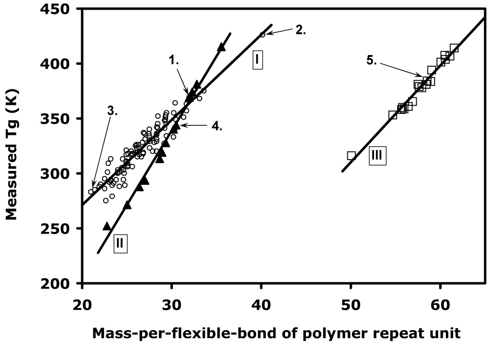
The experimental glass transition temperature plotted against the calculated mass-per-flexible-bond for all 132 polymers from the library disucssed in this work, showing class specific behavior. I. Polycarbonates and polyarylates (open circles); II. Poly(DTE-co-DT-co-PEG carbonate)s (filled triangles); III. Poly(I2DTEco- I2DT-co-PEG carbonate)s (open squares). The bold lines are linear fits (See Table 2 for fit coefficients). The numbers 1–5 refer to the polymer structures in Figure 3 and Table 1.
It can be seen in Figure 4 that the library can naturally be divided into three main classes (I, II, and III). This polymer class specific behavior has been observed and explained previously [16] and is a result of the different densities, steric hindrances and intermolecular interactions in different polymer classes. In this specific library, the three classes are the following: I) the XTR carbonate homopolymers and all the poly(DTR arylate)s; II) all poly(DTE-co-y% DT-co-z% PEGm carbonate)s; and III) all poly(I2DTE-co-y% I2DT-coz% PEGm carbonate)s, the linear fit coefficients of which are listed in Table 2.
Table 2.
Linear fit parameters obtained from equation (1) for the three polymer classes shown in Figure 5
| Polymer class | Linear fit parameters for Equation (1) | |||
|---|---|---|---|---|
| A | C | R2 | ||
| I | All polycarbonates and polyarylates | 7.7505 | 116.17 | 0.9050 |
| II | Poly(DTE-co-DT-co-PEG carbonate)s | 13.512 | −66.374 | 0.9889 |
| III | Poly(I2DTE-co-I2DT-co-PEG carbonate)s8.8031 | −130.02 | 0.9775 | |
The division of our library into three classes can be rationalized as follows: 1) PEG and iodine containing co- and terpolymers are estimated to have a lower and higher density, respectively, than pure XTR polymers that only contain aliphatic and aromatic groups, and the mass-per-flexible-bond approach does not account for this density difference resulting in a shift of the line towards high M/f values, as well as a change in slope; 2) iodine increases the molecular weight of monomers through its high atomic mass, while simultaneously decreasing the number of flexible bonds through steric hindrance, thereby increasing its M/f, again shifting the line towards high M/f values; and most importantly 3) the interchain hydrogen bonding in the three classes is of a different magnitude.
The hydrogen bonding interactions between the mobile PEG ether groups and the DT carboxylic acid groups in class II (the poly(DTE-co-DT-co-PEG carbonate)s) are expected to be strong, while in class III (the same polymers but iodinated) these interactions are most probably be much weaker due to steric hindrance and the hydrophobic nature of the bulky iodine substituents. The total absence of both PEG and free carboxylic acid groups in the polymers of class I decreases the hydrogen bonding interactions in these polymers to even lower levels. This explanation is supported by the changes in the slope of the fitted lines increases among the three classes (Table 2): I<III<<II (7.7505, 8.8031 and 13.512, respectively), which corresponds to an increase in intra and interchain interactions [18]. Furthermore, it can be concluded that the hydrophobic iodine substituents reduce the effect of the hydrophilic PEG blocks, as seen by the lower slope of class III that is closer to that of class I than II although a density effect cannot be excluded.
From Figure 4 and Table 2 it can be seen that the data scatter in class I is considerably larger that in classes II and III, as reflected by order of their increasing correlation coefficients: R2(I)<<R2(III)<R2(II) (0.9050, 0.9989, and 0.9775, respectively). There are a number of explanations for this data scatter: 1) the materials in classes II and III have been synthesized relatively recently compared to those in class I, leading to less operator dependent variations present in that sub library, e.g. experimental Tg values; 2) because the polyarylates are essentially alternating copolymers, they are extremely sensitive to stoichiometry and their molecular weights are therefore difficult to control, which might manifest itself in Tg variations; and 3) some of the polyarylates have been shown to display liquid crystalline like ordering behavior [18, 55–57], which will influence the Tg values through intermolecular hydrogen bonding, and these interactions that are not included in the mass-per-flexible-bond approach.
Tg prediction and evaluation of predictive accuracy
Despite the scatter in the available data in this polymer library, the correlations of Tg with M/f for these homo, co- and terpolymers are very good, suggesting that the proposed method can be used as a Tg prediction tool. A linear fit of the plot of the polymer’s Tg (in units of K) vs. (M/f) value can be used obtain the constants A and C of Equation (1). These values can then be used for the prediction of the Tg of a polymer by calculating its M/f value. However, in the present case all the Tg values in the library had already been measured and were available at the moment of the model construction. We therefore chose an a posteriori approach to evaluate the predictive accuracy of the proposed method.
An algorithm was written in Matlab (Math Works, Natick, MA; version 6.1.0.450, release 12.1) that selected, from a data set of n polymers, a construction set of k polymers, leaving n-k polymers as the test set. The data consisted of the M/f and Tg (in K) values of the polymers as the X and Y values, respectively. A least squares linear fit was performed on the Tg vs. M/f plot of the construction set polymers, giving the fit coefficients A and C for this set. These coefficients were then used to calculate the glass transition temperatures of each polymer in the test set via Equation (1). For each polymer in this test set we calculated ΔT, the absolute difference between the predicted and the experimentally measured Tg values. These individual ΔT values were averaged over the whole test set to give ΔT*, the average, absolute error in Tg prediction for that test set. Note that this value ΔT* result from only one of many possible combinations of choosing k out of n polymers to form this specific construction and test set. Thus, for reasons of completeness and objectivity we therefore generated all possible combinations of k out to n polymers that can make up that test set size, and averaged all the ΔT* values of those combinations to give ΔTav, the average error in Tg prediction for that specific test set (of size n-k). In order to investigate how many Tg values need to be known to accurately predict new Tg values, the size of the construction set was now varied from k=3 to k=n-1 with a step size of 1, leading to a progressively smaller test set in each case. The ΔTav values were calculated for all construction set sizes k, and the trend of ΔTav vs. k was investigated to establish the minimum construction set size (k) necessary to accurately predict new Tg values.
Accuracy of the prediction
In order to objectively evaluate the predictive accuracy of this method, an a posteriori data selection and analysis procedure, described in the experimental methods section, was employed. Figurea 5a to 5d show a selection of four representative plots of the predicted vs. measured glass transition temperature in the class of poly(DTE-co-y% DT-co-z% PEGm carbonate)s (13 data points) for four different sizes of the construction set k: 3, 4, 5, and 7. It should be noted that each plot represents one random selection from all possible combinations P of choosing k out of n values, for that construction set of size k. Increasing the construction set size obviously reduces the number of predicted values in the test set from 10 to 6. It is clear from these plots that increasing k from 3 to 7 gives more accurate prediction results for the test set, as seen from 9 the decreasing data point deviation of the predicted values from the line y=x that represents a perfect prediction. This fact is reflected in the average, absolute prediction error (ΔTav) associated with each plot that decreased from 6.6 to 5.3 K upon increasing k from 3 to 7. For small polymer classes (n≤15) all possible combinations P were selected and used to calculate the corresponding ΔTav values. However, for large classes (n>15) P becomes very large (the number of possible unordered combinations P to choose k polymers from a set of n values is given by P=n!/((k!(n-k)!), written as nCk). For example, using n=100 and taking half of the values for the construction set (i.e. 100C50) results in P~1029 different combinations of k out of n polymers. A computation of this magnitude is beyond the memory capacity of a regular personal computer, and in these cases we therefore reduced the number of data points by limiting the number of construction sets that were investigated. For large data sets the size of the construction set was therefore varied from k=10 to k=n-10 with a step size of 10. Additionally, instead of using all possible combinations P per construction set, we randomly selected only 2000 combinations from which ΔTav was calculated.
Figure 5.

The experimental Tg vs. predicted Tg for class I, the poly(DTE-co-DT-co-PEG carbonate)s (n=13) for four different sizes of the construction set k. a) k=3; b) k=4; c) k=5; d) k=7. The line Y=X indicates a perfect prediction. Note that each plot is one randomly selected combination out of many for choosing k out of 13 values.
For reasons of brevity we present the results of these calculations in Figure 6, as a plot of the average, absolute prediction error (dTav) vs. k for all three polymer classes. Note that k is expressed as the % of the available data points to better compare the behavior of the three data sets. This plot allows for the determination of the best attainable Tg prediction error in each class from the asymptotic value of ΔTav with increasing k, as well as the minimum size of the construction set necessary for accurate prediction (kmin). It can be seen that, while the value of ΔTav for polymer classes I and III levels off around 30 and 50%, respectively, that of class II seems to decreases continuously with k. This behavior is suspected to be due to the large data scatter in this polymer class. Table 3 lists the values of ΔTav at kmin. It can be seen that the average error in Tg prediction is 6.4, 5.3, and 3.7 K for series I, II, and III, respectively. These values are remarkably low considering the simplicity of the model, the large data scatter in the Tg vs. M/f plots, and the structural variety in the library. In fact, this accuracy is better than most of the results from (semi-) empirical Tg prediction methods found in the literature [30–43, 50].
Figure 6.

The evolution of the average, absolute error (ΔTav) in the predicted Tg values as a function of construction set size k for the three polymer classes discussed in this work. I. Polycarbonates and polyarylates (open circles); II. Poly(DTE-co-DT-co-PEG carbonate)s; (filled triangles); III. Poly(I2DTE-co-PEG carbonates’s (open squares).
Table 3.
The average, absolute error in the Tg values predicted by equation (1) for the three polymer classes found in Figure 1 at k=50%.
| Polymer class | Polymers | Set size | k mina | ΔTav: Average Tg prediction error (K) |
|---|---|---|---|---|
| I | All polycarbonates and polyarylates | 100 | 7b | 6.4 |
| II | Poly(DTE-co-DT-co-PEG carbonate)s | 13 | 7 | 5.3 |
| III | Poly(I2DTE-co-I2DT-co-PEG carbonate)s | 19 | 7 | 3.7 |
The minimum size of the construction set (in nr of X,Y pairs) necessary to obtain the best Tg prediction (lowest ΔTav) in that class
No asymptotic behavior, arbitrarily chosen value of k
Structure calculation from target Tg
Equation (1) can also be used in the reverse manner from the above approach, namely polymer structure prediction for a target Tg value when the fit coefficients A and C are known. Knowledge of the fit coefficients A and C, and the choice of a target Tg now lead to the identification of the polymer with an M/f value that corresponds to one desired composition or a range of polymer compositions in the case of terpolymers, allowing the best suitable material to be chosen. In the case of terpolymers, combination of Equation (1), (2) and the fact that the sum of mass fractions equals unity results in Equations (4a) and (4b)
| (4a) |
| (4b) |
where xMi is the mass fraction of the polymer repeat unit i; M is the molecular weight of the repeat unit (in g/mol); f is the number of flexible bonds in the repeat unit; (M/f)i is the mass-per-flexible-bond of the repeat unit; Tg is the targeted glass transition temperature of the polymer (in K); and A and C are polymer class specific constants.
This reverse approach will be illustrated with a specific example: the poly(DTE-co-DT-co-PEG1000 carbonate)s and the poly(I2DTE-co-I2DT-co-PEG1000 carbonate)s. Substitution of the appropriate M/f values of the monomers from Table 1 and the fit coefficients A and C from Table 2 for these two polymer 10 classes into the Equations (4a) and (4b) with subscripts 1, 2 and 3 replaced by DTE, DT and PEGm respectively. When adapted to classes II and III, we get Equations (5a) and (5b) for the poly(DTE-co-DT-co-PEG1000 carbonate)s and Equations (6a) and (6b) for the poly(I2DTE-co- I2DT-co-PEG1000 carbonate)s,
| (5a) |
| (5b) |
| (6a) |
| (6b) |
where xIxDTE is the mass fraction of the IxDTE monomer in the terpolymer (x being 0 or 1), xIxDT the mass fraction of the IxDT monomer, xPEG1000 the mass fraction of PEG1000, and Tg is the main glass transition temperature of the terpolymer (K). Equations (6a) and (6b), (7a), and (7b) were used to calculate the different terpolymer compositions that correspond to a target Tg, In this we chose 60 °C, and a number of these corresponding polymer compositions are listed in Table 4. In this specific example it is thus possible to smoothly change the polymer composition from 86/0/14 to 0/71/29 (in mass% DTE/DT/PEG1000) for poly(DTE-co-DT-co-PEG1000 carbonate)s and from 83/0/17 to 0/67/33 (in mass% I2DTE/I2DT/PEG1000) for the poly(I2DTE-co- I2DT-co-PEG1000 carbonate)s without affecting the Tg of 60 °C. The fact that the stiffer monomer I2DTE increases the Tg of the terpolymer is illustrated by the fact that this class can have a higher PEG1000 content than the corresponding non-iodinated polymer at the same IxDT content while maintaining its Tg of 60 °C. This makes it possible to tune the degradation rate, water uptake, protein adsorption and the cell-material interactions independently of the glass transition temperature, by proper choice of polymer type and composition within these two polymer classes.
Table 4.
Selected terpolymer compositions of poly(IxDTE-co-IxDT-co-PEG1000 carbonate)s that have a predicted Tg of 60°C. with Tg = 60°C (Mass%)
| DTE | DT | PEG1000 | I2 DTE | I 2 DT | PEG1000 | |
|---|---|---|---|---|---|---|
| 85.85 | 0 | 14.15 | 82.63 | 0 | 17.37 | |
| 73.72 | 10 | 16.28 | 70.22 | 10 | 19.78 | |
| 61.59 | 20 | 18.41 | 57.81 | 20 | 22.19 | |
| 49.46 | 30 | 20.54 | 45.41 | 30 | 24.59 | |
| 37.33 | 40 | 22.67 | 33.00 | 40 | 27.00 | |
| 25.20 | 50 | 24.80 | 20.59 | 50 | 29.41 | |
| 13.07 | 60 | 26.93 | 8.18 | 60 | 31.82 | |
| 0 | 70.78 | 29.22 | 0 | 66.59 | 33.41 |
It should be noted that the predicted values are dry Tg’s, plasticization by water of the hydrophilic PEG blocks is not taken into account, and it is likely that the extreme polymer compositions are beyond the predictive capacity of the current method. However, it is evident that this method has broad applications in polymer and (bio)material science in general, as it allows for the decoupling of the thermal (and perhaps mechanical) behavior of a terpolymer from its chemistry and surface energy.
Conclusions
The mass-per-flexible bond principle was used for the first time to devise a semi-empirical Tg prediction method that is applicable to polymers with any number of comonomers. A self consistent set of rules for the assignment of bond flexibility, applicable to any polymer structure, was given, as well as formulas for the calculation of the M/f values of co- and terpolymers. The method was validated by applying it to a 132-member L-tyrosine derived polymer library, containing a wide range of polymer structures. A plot of the experimental Tg vs. calculated M/f values yielded straight lines when the polymers were divided into different classes. This division was explained in terms of the different densities, steric hindrances and intermolecular interactions in each polymer class. An a posteriori predictive accuracy evaluation showed that average, absolute error between predicted and measured Tg ranged from 6.4 to 3.7 K for the three polymer classes investigated in this work. This accuracy is very good considering the data scatter and the large variety of functional groups present in this library, and it is better than most ab initio, molecular mechanics, or (semi-)empirical prediction methods found in the literature. Furthermore, the current method has the advantage of being considerably simpler to use than many of the existing methods. We showed that as little as seven Tg values can be used to accurately predict the Tg’s of other polymers in that class. Additionally it was shown that the proposed method can be used in the reverse manner: to calculate polymer structures that match a certain target Tg value based on the linear fit coefficients of a polymer class. This enables keeping the thermal (and perhaps the mechanical) behavior of a terpolymer constant while independently choosing its chemistry and surface energy.
In summary: we provided a simple, accurate, and universal method for both Tg prediction and polymer structure calculation from a few initial experimental Tg values. This method is likely to have broad applications in polymer and (bio)material science.
ACKNOWLEDGMENTS
We thank Dr. Anna Gubskaya and Dr. Paul Holmes for their helpful discussions. Funding for this work was provided by (i) RESBIO - The National Resource for Polymeric Biomaterials funded by the National Institutes of Health (NIH grant EB001046), (ii) by a collaboration with Professor Roth, funded by NIH grant GM065913, and (iii) by support from REVA Medical, Inc., San Diego, CA.
Footnotes
This is a PDF file of an unedited manuscript that has been accepted for publication. As a service to our customers we are providing this early version of the manuscript. The manuscript will undergo copyediting, typesetting, and review of the resulting proof before it is published in its final citable form. Please note that during the production process errors may be discovered which could affect the content, and all legal disclaimers that apply to the journal pertain.
References
- 1.Hoogenboom R. High-throughput experimentation, microwave irradiation, and grid-like metal complexes. Eindhoven: Technical University of Eindhoven; 2004. Expanding the polymer toolbox; p. 216. [Google Scholar]
- 2.Meier MAR, Schubert US. J. Mat. Chem. 2004;14:3289–3299. [Google Scholar]
- 3.Weber N, Bolikal D, Bourke SL, Kohn J. J. Biomed. Mater. Res. 2004;68A:496–503. doi: 10.1002/jbm.a.20086. [DOI] [PubMed] [Google Scholar]
- 4.Kholodovych V, Smith JR, Knight D, Abramson S, Kohn J, Welsh WJ. Polymer. 2004;45:7367–7379. [Google Scholar]
- 5.Smith JR, Kholodovych V, Knight D, Kohn J, Welsh WJ. Polymer. 2005;46(12):4296–4306. [Google Scholar]
- 6.Smith JR, Kholodovych V, Knight D, Welsh WJ, Kohn J. QSAR Comb. Sci. 2005;24:99–113. [Google Scholar]
- 7.Smith JR, Knight D, Kohn J, Rasheed K, Weber N, Kholodovych V, Welsh WJ. J. Chem. Inf. Comput. Sci. 2004;44:1088–1097. doi: 10.1021/ci0499774. [DOI] [PubMed] [Google Scholar]
- 8.Smith JR, Seyda A, Weber N, Knight D, Abramson S, Kohn J. Macromol. Rapid Commun. 2004;25:127–140. [Google Scholar]
- 9.Sharma RI, Kohn J, Moghe PV. J. Biomed. Mater. Res. 2004;69A:114–123. doi: 10.1002/jbm.a.20125. [DOI] [PubMed] [Google Scholar]
- 10.Zeltinger J, Schmid E, Brandom D, Bolikal D, Pesnell A, Kohn J. Biomaterials Forum (Official Newsletter of the Society for Biomaterials) 2004;26(1):8–24. [Google Scholar]
- 11.Tangpasuthadol V, Pendharkar SM, Kohn J. Biomaterials. 2000;21:2371–2378. doi: 10.1016/s0142-9612(00)00104-6. [DOI] [PubMed] [Google Scholar]
- 12.Tangpasuthadol V, Pendharkar SM, Peterson RC, Kohn J. Biomaterials. 2000;21:2379–2387. doi: 10.1016/s0142-9612(00)00105-8. [DOI] [PubMed] [Google Scholar]
- 13.Painter PC, Coleman MM. Fundamentals of Polymer Science. Basel: Technomic Publication AG; 1994. [Google Scholar]
- 14.Di Marzio EA. Polymer. 1990;31:2294–2298. [Google Scholar]
- 15.Schneider HA. Journal of Research of the National Institute of Standards and Technology. 1997;102(2):229–248. doi: 10.6028/jres.102.018. [DOI] [PMC free article] [PubMed] [Google Scholar]
- 16.Schneider HA. Polymer. 2005;46:2230–22237. [Google Scholar]
- 17.Schneider HA, Di Marzio EA. Polymer. 1992;33(16):3453–3461. [Google Scholar]
- 18.Schneider HA. J. Appl. Pol. Sc. 2003;88:1590–1599. [Google Scholar]
- 19.Mark J, Ngai K, Graessley W, Mandelkern L, Samulski E, Koenig J, Wignall G. Physical Properties of Polymers. Basel: Technomic Publications AG; 2004. [Google Scholar]
- 20.Tangpasuthadol V, Shefer A, Yu C, Zhou J, Kohn J. J. Appl. Polym. Sci. 1997;63(11):1441–1448. [Google Scholar]
- 21.Katajisto J, Linnolahti M, Pakkannen TA. Theor. Chem. Acc. 2005;113:281–286. [Google Scholar]
- 22.Ton TMT, Rode BM. Macromol. Theory Simul. 1996;5(3):467–475. [Google Scholar]
- 23.Paul W. AIP Conference Proceedings; 1992. pp. 145–154. [Google Scholar]
- 24.Wittkop M, Hoelzl T, Kreitmeier S, Goeritz D. J. Non-Cryst. Sol. 1996;201:199–210. [Google Scholar]
- 25.Boyd RH. Trends Polym. Sci. 1996;4(1):12–17. [Google Scholar]
- 26.Hamerton I, Heald CR, Howlin BJ. J. Mater. Chem. 1996;6(3):311–314. [Google Scholar]
- 27.Hamerton I, Howlin BJ, Klewpatinond P, Shortley HJ, Takeda S. Polymer. 2006;47:690–698. [Google Scholar]
- 28.Zhang M, Sundararaj U, Choi P. PMSE Preprints. 2004;91:1031–1032. [Google Scholar]
- 29.Abu-Sharkh BF. Comp. Theor. Pol. Sc. 2001;11:29–34. [Google Scholar]
- 30.Becker R, Neumann G. Plaste und Kautschuk. 1973;20(11):809–815. [Google Scholar]
- 31.Brown WM, Martin S, Rintoul MD, Faulon J-L. J. Chem. Inf. Model. 2006;46:826–835. doi: 10.1021/ci0504521. [DOI] [PubMed] [Google Scholar]
- 32.Camacho-Zuniga C, Ruiz-Trevino FA. Ind. Eng. Chem. Res. 2003;42:1530–1534. [Google Scholar]
- 33.Carro AM, Campisi B, Camelio P, Phan-Tan-Luu R. Chemometrics and Intelligent Laboratory Systems. 2002;62:79–88. [Google Scholar]
- 34.Cypcar CC, Camelio P, Lazzeri V, Mathias LJ, Waegell B. Macromolecules. 1996;29:8954–8959. [Google Scholar]
- 35.Garcia-Domenech R, De Julian-Ortiz JV. J. Phys. Chem. B. 2002;106:1501–1507. [Google Scholar]
- 36.Hopfinger AJ, Koehler MG, Pearlstein RA. J. Pol. Sc., B. Phys. 1988;26:2007–2028. [Google Scholar]
- 37.Joyce SJ, Osguthorpe DJ, Padgett JA, Price GJ. J. Chem. Soc. Faraday Trans. 1995;91(16):2491–2496. [Google Scholar]
- 38.Katritzky AR, Rachwal P, Wah Law K, Karelson M, Lobanov VS. J. Chem. Inf. Comput. Sci. 1996;36(4):879–884. [Google Scholar]
- 39.Kreibich UT, Batzer H. Angew. Makromol. Chemie. 1979;83:57–112. [Google Scholar]
- 40.Mattioni BE, Jurs PC. J. Chem. Inf. Comput. Sci. 2002;42:232–240. doi: 10.1021/ci010062o. [DOI] [PubMed] [Google Scholar]
- 41.Van Krevelen DW. Properties of polymers. Amsterdam: Elsevier; 1976. [Google Scholar]
- 42.Weyland HG, Hoftijzer PJ, Van Krevelen DW. Polymer. 1970;11(2):79–87. [Google Scholar]
- 43.Zhang L, Zhao D, Huang Y. Chinese J. Pol. Sc. 2002;20(2):25–30. [Google Scholar]
- 44.Yu X, Wang X, Li X, Gao J, Wang H. Macromol. Theory Simul. 2006;15:94–99. [Google Scholar]
- 45.d'Acunzo F, Kohn J. Macromolecules. 2002;35:9360–9365. [Google Scholar]
- 46.Ertel SI, Kohn J. J. Biomed. Mater. Res. 1994;28:919–930. doi: 10.1002/jbm.820280811. [DOI] [PubMed] [Google Scholar]
- 47.Fiordeliso J, Bron S, Kohn J. J. Biomater. Sci. (Polym. Ed.) 1994;5(6):497–510. [PubMed] [Google Scholar]
- 48.Kohn J. Trends Polym. Sci. 1993;1(7):206–212. [Google Scholar]
- 49.Pulapura S, Kohn J. Biopolymers. 1992;32:411–417. doi: 10.1002/bip.360320418. [DOI] [PubMed] [Google Scholar]
- 50.Yu C, Kohn J. Biomaterials. 1999;20(3):253–264. doi: 10.1016/s0142-9612(98)00169-0. [DOI] [PubMed] [Google Scholar]
- 51.Brocchini S, James K, Tangpasuthadol V, Kohn J. J. Amer. Chem. Soc. 1997;119(19):4553–4554. [Google Scholar]
- 52.Fox TG, Flory PJ. J. Appl. Phys. 1950;21:581. [Google Scholar]
- 53.Fox TG, Flory PJ. J. Polym. Sci. 1954;14:315. [Google Scholar]
- 54.Sousa A, Schut JA, Kohn J, Libera M. Macromolecules. 2006;39(21):7306–7312. [Google Scholar]
- 55.Jaffe M, Ophir Z, Collins G, Recber A, Yoo S, Rafalko J. Polymer. 2003;44:6033–6042. [Google Scholar]
- 56.Jaffe M, Ophir Z, Pai V. Thermochimica Acta. 2003;396:141–152. [Google Scholar]
- 57.Jaffe M, Pai V, Ophir Z, Wu J, Kohn J. Pol. Adv. Tech. 2002;13:926–937. [Google Scholar]