Optimization of linear disorder predictors yields tight association between crystallographic disorder and hydrophobicity

Abstract

X-ray crystallographic protein structures often contain disordered regions that are observed as missing electron density. Diffraction data may give little or no direct evidence as to the specific nature of disordered regions. We have developed a weighted window-based disorder predictor optimized using crystallographic data. Performance of a predictor is strongly influenced by chain termini. Optimized score adjustment values for amino- and carboxy-terminal positions demonstrate a simple, monotonic relationship between disorder and residue distance from termini. This optimized disorder predictor performs similarly to DISOPRED2 on crystallographically disordered regions. Data-optimized residue disorder propensities show strong linear correlation with experimentally determined amino acid transfer energies between water and hydrogen-bonding organic solvents, which primarily reflect residue hydrophobicity (exemplified by the Nozaki-Tanford hydrophobicity scale). Disorder propensities do not correlate as well with transfer energies between water and apolar solvents, which primarily reflect a different hydropathic property: residue hydrophilicity (also reflected by the Kyte-Doolittle hydropathy scale). Our results suggest that while hydrophobic side-chain interactions are primarily involved in determining stability of the folded conformation, hydrogen bonding, and similar polar interactions are primarily involved in conformational and interaction specificity.

For over fifty years, scientists have discussed how fundamental physical properties of amino acids might relate to protein structure (Waugh 1954; Kauzmann 1959). Yet significant gaps remain in our understanding of how the simple physical properties of amino acids dictate the complex structural characteristics of proteins (Chandler 2005). Protein disorder, or the lack of consistent folded structure, represents one such characteristic.

To help evaluate disorder in proteins, a number of predictors have been developed (Galzitskaya et al. 2006a,b; Han et al. 2006; Vullo et al. 2006; Wang and Donald 2006; Dosztanyi et al. 2007; Hirose et al. 2007; Shimizu et al. 2007; Sickmeier et al. 2007; Sugase et al. 2007). The DisProt Website (Sickmeier et al. 2007), at http://www.disprot.org, provides links to several predictors. Some predictors utilize various predetermined residue-type characteristics to make predictions (Linding et al. 2003b; Coeytaux and Poupon 2005; Dosztanyi et al. 2005a,b; Prilusky et al. 2005; Peng et al. 2006), while other predictors use “machine learning” of disorder data to develop complex networks of parameters (Romero et al. 1997; Linding et al. 2003a; Vucetic et al. 2003; Ward et al. 2004; Cheng et al. 2005; Yang et al. 2005) that are not easily related to physical terms (Lise and Jones 2005). Ferron et al. (2006) provide an informative review of disorder predictors.

We have developed data-optimized disorder predictors that use a weighted sliding-window algorithm to calculate position-dependent disorder scores. Using such an approach allows position-dependent predictions that can account for local influence of adjacent residues within the span of the window. Some predictors specifically address disorder-prone chain-terminal regions (Li et al. 1999; Ward et al. 2004). We use a simple method to address predictions at termini, which reveals similar behavior of disorder at each terminus. As opposed to predictors that utilize complex networks of parameters, the optimized parameters from our window-based predictors provide insight into disorder. Thus, optimized disorder parameters are compared with amino acid properties to provide insight into the physical underpinnings of disorder.

Several numerical indices represent physicochemical properties of amino acids measured either experimentally using individual amino acids or statistically using information available in protein structures. Many of these indices have been assembled into an AAindex database (Kawashima and Kanehisa 2000) and have been classified into hierarchical clusters of similar properties (Tomii and Kanehisa 1996). Numerical indices reflecting various properties have been used in predicting disorder, such as coil propensity (Linding et al. 2003b), hydropathy (Prilusky et al. 2005), and interaction energy (Dosztanyi et al. 2005b). Property scales may also be derived by training predictors on disorder data (Weathers et al. 2004).

Among properties associated with disorder, “hydrophobicity” is commonly mentioned (Uversky et al. 2000; Williams et al. 2001; Linding et al. 2003a; Dosztanyi et al. 2005b; Peng et al. 2006). However, the term hydrophobicity has been loosely applied to widely varying scales (Creighton 1993, 2002), such as those of Kyte and Doolittle (1982) and Nozaki and Tanford (1971). These scales display only marginal correlation. Thus, the implications of associations between disorder and hydrophobicity are unclear. Our amino acid disorder propensities demonstrate a strong linear correlation with experimentally derived transfer energies between polar organic and aqueous phases, while showing a weaker correlation with transfer energies between apolar organic solvent and water (Radzicka and Wolfenden 1988). We therefore discriminate between two distinct amino acid properties that describe side-chain affinities to organic solvents.

The first property is characterized by the transfer energies between water and polar organics, for example, alcohols. In this case, both solvents offer hydrogen-bonding interactions, but only the organic phase offers hydrophobic protection. Assuming that hydrogen-bonding capacity is fully realized in both phases, partitioning is driven by the hydrophobic effect, and we term this property “hydrophobicity.” The second property refers to transfer energies between water and nonpolar organics, for example, cyclohexane. In this case, hydrogen bonds can be formed in water but not in cyclohexane. Thus, the dominant contribution to partitioning is hydrogen-bond formation, and we term this property “hydrophilicity.” In our terminology, hydrophobicity and hydrophilicity are not two polar opposites but represent two different, although not fully uncorrelated, amino acid properties. The two properties are distinguishable by the type of environment that surrounds amino acids in partitioning experiments, with the former describing partitioning between polar solvent and water, and the latter playing a dominant role in partitioning between nonpolar solvent and water. We discuss how the particular pattern in our data-optimized parameters helps clarify the relationship between this more precisely defined property of hydrophobicity and disorder.

Results and Discussion

Predictor performance

Figure 1 compares performance of our predictors (including simple sequence and profile-based predictors, with and without tail adjustments) with DISOPRED2 (Ward et al. 2004), a support vector machine (SVM)/neural network-based predictor of disorder also developed using crystallographic data that uses PSI-BLAST-generated sequence alignment profiles (Altschul et al. 1997) in its prediction. Some recent papers have compared disorder predictor performance with probability excess measurements (Yang et al. 2005; Esnouf et al. 2006; Su et al. 2006). Probability excess values typically depend on the cutoff score used in making a binary decision, and the probability excess reflects a single point on the receiver operating characteristic (ROC) curve. We use traditional full ROC curves for performance comparison.

Figure 1.

Performance comparison. DISOPRED2 serves as a reference. (A) Average ROC curves, including terminal residues in performance analysis. (B) “Average” ROC curves, excluding 30 terminal residues in performance analysis. (C) Differences between performance of profile with tail adjustments predictor and DISOPRED2 on individual testing data subsets. ROC scores at different cutoffs obtained by subtracting DISOPRED2's ROC score from the profile with tail adjustments predictor's ROC score (see Methods for explanation of ROC scores). (D) Average ROC curve for optimized simple sequence predictor (Sequence) compared with performance substituting various pre-existing scales for disorder propensities (see abbreviation footnote and body of text for further details). Areas under ROC curves: Sequence, 0.779; LOR, 0.771; Ky/Do, 0.697; Ho/Wo, 0.689; Ru/Li, 0.637; Ch/Fa, 0.621. (Area under curve for random predictions = 0.5.)

As with DISOPRED (Jones and Ward 2003; Ward et al. 2004), use of profiles enhances overall performance compared with using simple sequence (Fig. 1A). However, the improvement primarily occurs in the prediction of disorder in chain terminal regions, which make up more than half of the disorder in data sets (see Methods). When performance on these terminal residues is excluded from analysis, the simple sequence-based predictor performs comparably with the profile predictor and DISOPRED2 (Fig. 1B). Furthermore, when terminal residues are included in performance analysis, our treatment of sequence ends substantially narrows the performance gaps between the simple predictor, the profile predictor, and DISOPRED2 (Fig. 1A).

Although the predictors with tail adjustments are similar in overall performance to DISOPRED2, variations in performance on cross-validation data subsets reveal that predictors behave differently (Fig. 1C). Data subset 3 appears to be substantially affected by the Structural Classification of Proteins (SCOP) family “RNA-polymerase beta-prime” (ID = 64490), which contains sizeable disordered regions. Two of the chains contain long, imperfect repeats of the sequence, “PSTPSYS,” a pattern that may be detected somehow by DISOPRED2.

Optimized parameters

Optimized predictor parameters (between 55 and 119, depending on the predictor) include sliding window weights, amino acid disorder propensities, and tail adjustment values (Fig. 2). Parameters optimized on different cross-validation data sets showed high consistency (data not shown). Window weight parameters form a bell-shaped curve, showing the relative degree to which nearer and farther positions are appropriately taken into account in predicting crystallographic disorder. Positions on the C-terminal side weighted slightly more than their N-terminal counterparts for both profile and simple sequence predictors (Fig. 2A). The reason for this mild asymmetry is unclear.

Figure 2.

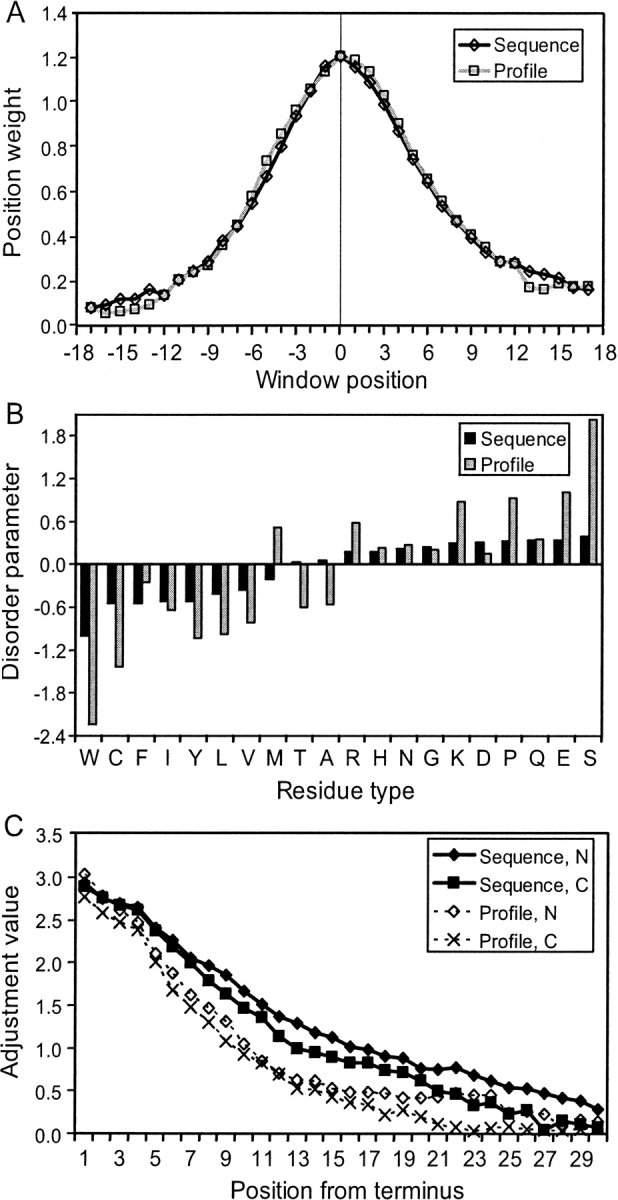
Predictor parameters. (A) Optimized weights are depicted for each position in the sliding window as open diamonds. The calculated disorder score is assigned to the residue position (0) indicated by a vertical line. (B) Simple sequence predictor disorder values are in black bars, and profile predictor values are in gray bars. Negative values indicate more order than average, and positive values indicate more disorder than average. LORs are based on residue frequency in disorder data sets. (C) Tail adjustment values, which are added to disorder scores at positions near amino and carboxy termini when the tail adjustment option is used.

Disorder values for the sequence- and profile-based predictors follow different patterns (Fig. 2B), but for both predictors, tryptophan is the most order-associated residue type, and serine is the most disorder-associated standard residue type. In the simple sequence predictors, threonine and alanine, with disorder values close to 0, have approximately average ordering propensity; W, C, F, I, Y, L, V, and M display less than average disorder propensity; and R, H, N, G, K, D, P, Q, E, and S display higher than average disorder propensity.

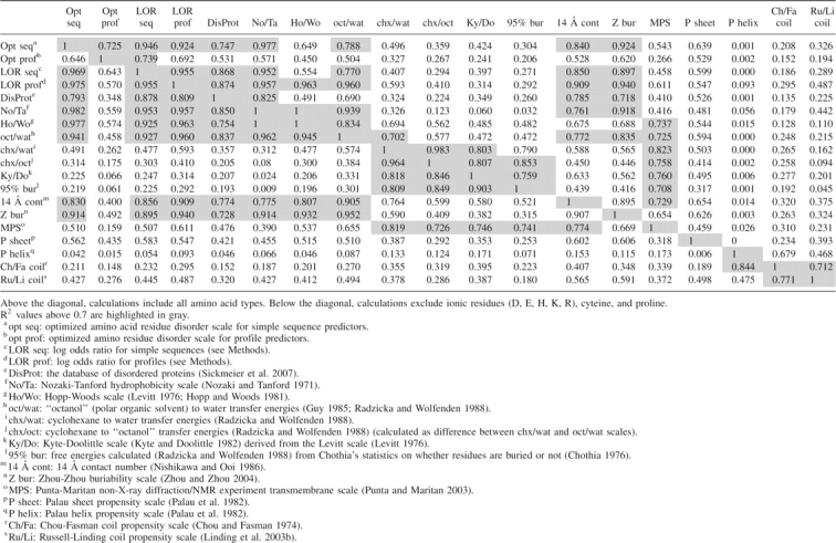
Simple sequence predictor disorder propensities (Table 1) correlate strongly with statistical residue disorder propensities (log odds ratios; R² = 0.946; Table 2), but a similar relationship is not seen for profiles (Table 2), indicating that statistical derivation of parameters does not always produce the same results as optimization. Of note, the calculation of log odds ratios (LORs) closely resembles that of free energy (ΔG = lnK), and LORs are additive (behave linearly).

Table 1.

Simple sequence predictor disorder values for common residue types, selenomethionine (sM), and N-terminal methionine (nM)

Table 2.

Correlations (R²) for selected scales

Tail adjustments are optimized in conjunction with composition-based disorder scoring and with the exclusion of polyhistidine tag influence (see Methods), thus removing confounding effects that might result from sequence bias at termini. The tail adjustments thus produced demonstrate that disorder approximately follows a simple, monotonic function of distance from the terminus that is equal for N- and C-termini (Fig. 2C), which may be the result of decreased constraint at chain termini. Tail adjustment values for the first three positions are negatively displaced because of the exclusion of disordered stretches shorter than four residues from optimization performance measures (see Methods).

Disorder propensity and hydrophobicity

Table 1 lists disorder propensities for the simple sequence predictor. Other groups have found similar scales in association with disorder (Williams et al. 2001; Linding et al. 2003a; Weathers et al. 2004). Substituting optimized parameters with rationally selected parameter scales in the simple disorder predictor allows comparison of different indices in predicting crystallographically disordered regions (Fig. 1D), including some indices utilized by available disorder predictors (Linding et al. 2003b; Prilusky et al. 2005; Peng et al. 2006). When substituted for optimized disorder propensities, predetermined coil propensity scales (Ru/Li: Russell-Linding propensity scale) (Linding et al. 2003b) (Ch/Fa: Chou-Fasman coil propensity scale) (Chou and Fasman 1974) do not perform as well in our sliding-window predictor at discriminating crystallographically disordered regions (Fig. 1D, purple- and olive-colored ROC curves). The Kyte-Doolittle scale (Ky/Do) (Kyte and Doolittle 1982) and the Hopp-Woods scale (Ho/Wo; derived from the Levitt scale) (Levitt 1976; Hopp and Woods 1981) yield better, but still suboptimal, performance (Fig. 1D, orange- and cyan-colored ROC curves). Predictions using LORs approach those of the optimized disorder propensities. In agreement with this observation, calculated LORs display strong correlation to optimized disorder propensities (R² = 0.946, Table 2).

Several structure-derived scales show strong correlations to disorder propensity (Table 2). A residue “buriability” scale (Z bur) (Zhou and Zhou 2004) displays the highest correlation to disorder (Z bur, R² = 0.924), while a residue interactivity scale (Bastolla et al. 2005) is ranked second (R² = 0.909). Other high-ranked scales measure contacts within a 14 Å sphere (Nishikawa and Ooi 1986) (14 Å cont, R² = 0.840) and nonbonded interactions for residues well separated in sequence (Oobatake and Ooi 1977) (R² = 0.837). Another amino acid stability scale (Vihinen et al. 1994), which was optimized on crystal structure temperature factor data using a sliding-window averaging technique, displays good correlation (R² = 0.865). Finally, structure-based hydrophobicity scales calculated for different protein classes (Cid et al. 1992) correlate with our optimized disorder values (R² = 0.839 for α/β, R² = 0.834 for β, and R² = 0.831 for all averaged). Overall, these scales suggest a relationship between order and the degree to which a residue tends to come into contact with other residues in existing protein structures (Williams et al. 2001; Dosztanyi et al. 2005b). Of note, our disorder propensities also correlate reasonably well with statistical disorder propensities calculated from the DisProt database (Sickmeier et al. 2007), with R² = 0.747 for all residues.

Among experimentally derived scales, disorder values correlate with polar organic solvent to water side-chain transfer energies (oct/wat; Fig. 3A, R ² = 0.788) (Guy 1985; Radzicka and Wolfenden 1988). Because of satisfied hydrogen-bonding potential in both partitions, these transfer energies reflect the strength of the hydrophobic effect. In contrast, cyclohexane to water transfer energies (chx/wat) (Radzicka and Wolfenden 1988) show a weaker relationship to disorder propensities (Fig. 3B, R² = 0.496). Because of an absence of hydrogen-bonding potential in one partition (chx), such a scale tends to reflect the preference of an amino acid to form hydrogen bonds with water or to “like” water (hydrophilicity). The transfer energy scales show that the relative hydrophobicity of an amino acid residue depends on the nonaqueous reference solvent, and they reflect the general diversity of scales that can be considered to be hydrophobic.

Figure 3.

Comparison of optimized disorder values with selected amino acid indices. Numerical values reported for each amino acid (labeled according to residue type) in various scales. (A) Octanol to water transfer energies (Guy 1985; Radzicka and Wolfenden 1988). (B) Cyclohexane to water transfer energies (Radzicka and Wolfenden 1988). (C) Nozaki-Tanford (Nozaki and Tanford 1971) side-chain transfer energies; glycine, as the reference amino acid, is given a value of 0. (D) Kyte-Doolittle hydropathy (Kyte and Doolittle 1982). (E) Hopp-Woods scale (Hopp and Woods 1983) (derived, in part, from Nozaki-Tanford scale). (F) Russell-Linding coil propensities (Linding et al. 2003b) are plotted against optimized disorder values. Ionic residues, Cys and Pro, are marked by open diamonds.

Scales comparable to the oct/wat transfer energies display similar tight correlations to disorder. For example, the incomplete hydrophobicity scale of Nozaki and Tanford (1971) (No/Ta), which reflects calculated side-chain free energies of transfer primarily between ethanol and water, is strongly correlated with disorder (Fig. 3C, R² = 0.977, missing 8 residues). The No/Ta scale excludes several side-chain types that might be expected to display special behavior, such as ionic residues, proline, and cysteine. However, a more complete (and inverted) version of this scale (Ho/Wo) used to predict protein epitopes also exhibits a linear correlation (Fig. 3E, R² = 0.649). In fact, this scale shows a clear linear relationship with disorder values for uncharged residues (R² = 0.910, excluding R, K, D, and E). Other scales reflective of the chx/wat transfer energies, such as Kyte-Doolittle (Ky/Do) hydropathies for predicting transmembrane segments, correlate weakly with our disorder parameters (Fig. 3D, R² = 0.424).

As previously described (Linding et al. 2003a), optimized disorder values are not well correlated with coil propensity: The strongest association found for this scale type being the Russell-Linding (Ru/Li) scale (Linding et al. 2003b) (R² = 0.326, Table 2). One might hypothesize that disorder is related to backbone flexibility and that glycine and perhaps small, nonbulky residues such as alanine promote disorder through their decreased steric hindrance of backbone motion. However, backbone flexibility does not appear to be a significant causal factor. Proline is conformationally limited yet is relatively disorder promoting. Glycine, on the other hand, is highly flexible but does not deviate substantially from the hydrophobicity trend.

Ionic residues do not consistently follow a linear relationship in hydrophobicity/disorder plots (e.g., Fig. 3A,E). Such residues pose specific problems for effectively measuring hydrophobicity in experimental settings. Partitioning experiments may not yield accurate hydrophobicities for ionic residues: Water has a stronger dielectric constant than polar organic solvents and is better able to accommodate charge; additionally, transfer energies depend on the solution pH (which affects solute charge) and on any special adjustments (Radzicka and Wolfenden 1988) made in calculations. In contrast to relatively long-range ionic interactions with surrounding solvent, hydrogen bonding and other polar solvent–solute interactions primarily involve close contacts. It is reasonable to conclude that aqueous and polar organic phases each offer interactions of approximately equivalent strength to the hydrogen-bonding moieties on amino acid side chains and that the predominant difference between solvation energies in aqueous and polar organic solution for nonionic amino acid side chains comes specifically from the hydrophobic effect.

Proline and cysteine also pose as special cases in considering hydrophobicity/disorder distributions. Cysteine and proline are not included in the oct/wat transfer energies. Wimley et al. (1996) offer values for all 20 standard amino acid types based on experiments using AcWL-X-LL pentapeptide constructs, but intramolecular interactions with large, hydrophobic side chains present a confounding factor in these experiments. The Levitt scale (Levitt 1976) (on which the Hopp-Woods scale is based) (Hopp and Woods 1981) provides interpolated hydrophobicities for nonionic residues not found in the Nozaki-Tanford scale (Nozaki and Tanford 1971). In the Levitt scale, the only nonionic residues that substantially deviate from the disorder/hydrophobicity trend are proline and cysteine. Proline has a higher disorder propensity than expected from its hydrophobicity, and cysteine has a lower than expected disorder propensity. Proline lacks the primary amine found in all other residues because of its cyclic side-chain binding the backbone nitrogen. This distinction makes proline less polar and restricts rotation about the ϕ torsion angle in protein structures. The rigid proline backbone often acts as a secondary structure disruptor for α-helices (Richardson 1981) and as a β-turn promoter (Chou and Fasman 1974), preventing it from occurring in the middle of secondary structures. The sulfhydryl group of cysteine can form stabilizing disulfide bonds with other cysteine residues and forms relatively weak hydrogen bonds with water.

A hydropathic spectrum reflects protein structure characteristics

Amino acid scales often represent a difference between two states. For example, disorder propensities compare the incidences of amino acid residue types in the disordered state versus the ordered state. The hydrophobic effect and hydrogen-bonding interactions make separate contributions to energetic differences between two states. Certain scales (such as disorder propensities) that quantify the difference between two structural states may be broken down into energetic components that are specifically attributable to the hydrophobic effect (“hydrophobic component”) and/or specifically attributable to polar, hydrogen bonding, or ionic interactions (“hydrophilic component”).

Whereas polar organic phases (such as wet octanol, ethanol, or methanol) and water largely differ because of the hydrophobic effect (for nonionic residues, as explained above), cyclohexane and octanol differ primarily in polar and hydrogen-bonding interactions. (Subtracting oct/wat energies from chx/wat energies produces the chx/oct scale [cyclohexane to octanol transfer energies]) (Radzicka and Wolfenden 1988.) Oct/wat hydrophobicities and chx/oct hydrophilicities correlate in part because of polar moieties that both reduce hydrophobicity and increase hydrophilicity. Despite some similarity, however, the oct/wat and chx/oct scales show that residue hydrophobicities and hydrophilicities follow distinct patterns (and that the absolute variance in hydrophilicities is larger than that of hydrophobicities).

Correlations with the oct/wat and chx/oct scale were calculated for various structural propensity scales. Excluding ionic residues, C and P, the oct/wat scale contains neither C nor P (Guy 1985; Radzicka and Wolfenden 1988). The curved line in Figure 4A represents correlations for all perfect, positive linear combinations of oct/wat and chx/oct. The proximity of a scale to this line reflects how well the property can be explained by a combination of the hydrophobic and hydrophilic patterns. Different positions along the spectrum are associated with different protein structural aspects: the hydrophobic end with crystallographic disorder and residue “buriability” (Zhou and Zhou 2004) (opt dis and Z bur, respectively, Fig. 4A), the middle with transmembrane helix potential (MPS: Punta-Maritan non-X-ray diffraction/NMR experiment transmembrane scale; Fig. 4A) (Punta and Maritan 2003), and the hydrophilic end with deep residue burial (Chothia 1976; Radzicka and Wolfenden 1988) (95% bur: free energies calculated from Chothia's statistics [Chothia 1976] on whether residues are buried or not; Fig. 4A). Kyte and Doolittle (1982) used water-vapor transfer energies and residue burial results of Chothia (1976) as well as some manual adjustment to develop their well-known hydropathy scale, which falls at the hydrophilic end of the spectrum. For predictions utilizing hydrophilicity (e.g., transmembrane predictions), the experimental chx/oct scale may offer improvement over Ky/Do.

Figure 4.

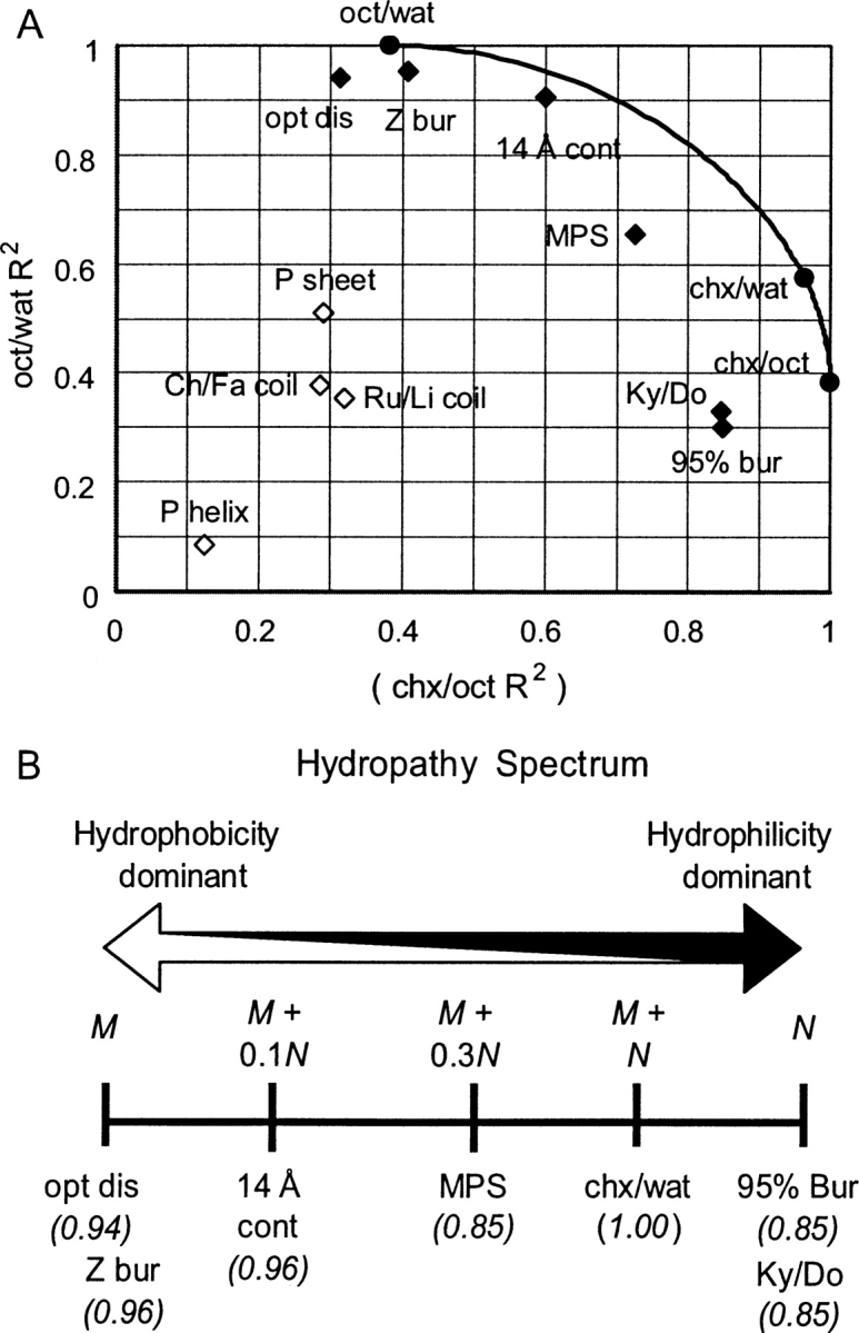
Hydropathy spectrum. (See abbreviation footnote and body of text for explanation of abbreviations.) (A) The relative degree of hydrophobic and hydrophilic components of various scales are approximated by calculating R² values (calculated excluding C, P, H, R, K, D, E) against octanol/water (oct/wat) partitioning energies (Guy 1985; Radzicka and Wolfenden 1988) on the Y-axis and cyclohexane/octanol (chx/oct) partitioning energies (Radzicka and Wolfenden 1988) on the X-axis, respectively. The curved line represents correlations for perfect, positive linear combinations of the oct/wat and chx/oct scales. Values for scales that can be largely explained by hydropathy fall near the curve and are represented by black diamonds. Values for the remaining scales are represented by open diamonds. (B) Locations of different scales along the hydropathy spectrum are represented by a linear combination of the oct/wat scale (M) and the chx/oct scale (N) that produces a near-maximum correlation with the scale, thus estimating the relative degrees to which the hydrophilic and hydrophobic components are present, respectively (the general magnitude of N is greater than that of M). Below the name of each scale, in italics, is the strength of association (R²) of that scale with the respective linear combination of M and N noted above it.

The hydropathic spectrum suggests that statistics discerning between fully (or almost fully) buried residues and residues that are more surface exposed reflect a strong influence from hydrophilic tendencies (95% bur vs. chx/wat, R² = 0.790, Table 2) (Radzicka and Wolfenden 1988) not the hydrophobic tendencies (95% bur vs. oct/wat, R² = 0.472, Table 2). This preference is illustrated in the position of the 95% burial scale near the extreme hydrophilic portion of the spectrum (95% bur, Fig. 4B). This position suggests that the environment in the extreme interior of a protein resembles cyclohexane, while the surface environment resembles an amphipathic solvent. Williams et al. (2001) found another scale related to surface proximity (14 Å cont) to be the best among several scales in discriminating between disorder and order. Indeed, comparing this scale with our disorder propensities yields a good correlation (R² = 0.840, Table 2), and the contact scale falls relatively close to our disorder propensities on the hydropathic spectrum (14 Å cont, Fig. 4). The contact number scale somewhat resembles the residue buriability scale, which falls the closest to disorder on the hydropathic spectrum scale (Z bur, Fig. 4).

Propensities to form secondary structures such as α-helices (P helix: Palau helix propensity scale) (Fig. 4A; Palau et al. 1982), β-strands (P sheet: Palau sheet propensity scale) (Fig. 4A; Palau et al. 1982), or coils (Ch/Fa and Ru/Li, Fig. 4A) do not appear to be explained well by hydropathy. Williams et al. (2001) found β-strand propensity to be somewhat useful in predicting disorder. However, our optimized disorder parameters do not display as strong a strong correlation with this characteristic (R² = 0.639, Table 2) as they do with hydrophobicity or residue burial. Disorder and strand propensity seem to be indirectly linked by a common association with hydrophobicity (R² = 0.594 for P sheet and oct/wat, Table 2), which might explain this relative degree of correlation. Positioning of β-strand propensity and α-helix propensity scales near coil propensity scales on the hydropathy spectrum (Fig. 4A) suggests that the capacity for a residue to form secondary structure is substantially affected by nonhydropathic influences. For example, side-chain branching tends to dictate presence in strands (Street and Mayo 1999; Pal and Chakrabarti 2000). Thus, secondary structure is more influenced by the specific size and shape of residues, while disorder is mainly influenced by the degree to which a residue tends to avoid interaction with water.

Rose et al. (1985) showed that average areas buried for different side chains in folded structures are associated with Nozaki-Tanford hydrophobicities, a simplified interpretation being that hydrophobic parts of side chains tend to be protected and hydrophilic parts exposed to water during folding. This interpretation helps explain the correlation of disorder propensities with various structurally derived scales (Oobatake and Ooi 1977; Nishikawa and Ooi 1986; Zhou and Zhou 2004; Bastolla et al. 2005). The tight disorder/surface burial/hydrophobicity correlations relate disorder propensity to both the structural property of surface burial and the physicochemical property of hydrophobicity. This relationship suggests that residues partition from an ordered state at the protein surface (octanol like) to a disordered state in the surrounding solution (water like). With relatively equal hydrogen-bonding potentials in the two states, a residue can transition into solution when a decrease in the entropy of water (due to exposed hydrophobic surface) (Butler 1937) is overcome with an increase in entropy from becoming disordered. In this case, a residue's hydrophobicity drives partitioning between surface (ordered) and solution (disordered).

Conclusions

Our sequence and profile disorder predictors with tail adjustments perform comparably with DISOPRED2. Although other predictors may yield better predictions in certain circumstances, our sequence-based predictor offers a simple, well-optimized predictor that avoids unknown bias toward special cases and may be useful as a step in a larger bioinformatic sequence analysis. It is useful to know how predictors perform on both internal and chain-terminal sequence regions (Fig. 1).

The disorder that commonly occurs at chain termini (see Table 3) is explained by lack of chain constraint (cysteine, on the other hand, increases constraint through disulfide bonding). Disorder tendency monotonically decreases as position moves away from the terminus in a manner that is essentially independent of whether the amino or carboxyl terminus is involved (Fig. 2C).

Table 3.

Data set statistics

Prior research has discussed patterns in disordered protein sequences (Vucetic et al. 2003; Lise and Jones 2005). Others have characterized amino acids in subsets (Li et al. 2000; Weathers et al. 2004; Ferron et al. 2006; Han et al. 2006; Su et al. 2006), for example, disorder-promoting, order-promoting, disorder-neutral. However, our data suggest that much of the variance in disorder behavior among different types of amino acids is reduced quantitatively, at a more fundamental level, by the hydrophobic effect (Butler 1937) alone, and that the transfer of a residue from an amphipathic environment to an aqueous environment (oct/wat) mimics the transfer of a residue from a position offering both hydrophobic and, if needed, hydrogen-bonding interactions (e.g., the protein surface) to a more solvated state (order/disorder transition). Residues with less hydrophobic character have a greater tendency to partition away from the protein and into the surrounding solvent.

In contrast with the hydrophobic effect, our data do not demonstrate a strong direct relationship with hydrogen-bonding interactions, secondary structure, or intrinsic backbone flexibility. Scales that are moderately associated with hydrophobicity (such as the Kyte-Doolittle scale) (Kyte and Doolittle 1982) may be used to predict disorder, but their discriminatory power is not always optimal (Fig. 1D). Other sequence determinants of disorder include cysteine, which forms disulfide bonds, and proline, with a backbone structure that enforces an extended conformation. The degree to which independent positive or negative charges affect disorder is not known, although our data suggest it is relatively small.

Similar patterns of disorder have been found by other researchers (Linding et al. 2003b; Weathers et al. 2004), which include noncrystallographic data sets (Williams et al. 2001). Thus, a hydrophobicity-based model of disorder is probably applicable beyond crystallographic disorder. Our optimized parameters also correlate (R² = 0.747; see Table 2) with a curated disorder data set provided by DisProt that also includes disordered regions from noncrystallographic data sets. However, distinct patterns may occur in long disordered regions (Peng et al. 2006). In fully unfolded chains, intrinsic conformation (or lack thereof) may become a more important factor in addition to stability, which may explain, beyond window size, why FoldIndex, which uses Kyte-Doolittle hydropathies, performs substantially better on fully disordered sequences than on crystallographic disorder (Esnouf et al. 2006).

As recently noted, “stability and conformation are not synonymous” (Rose et al. 2006). In contrast with hydrophobic groups, hydrogen-bonding groups do not play a significant role in stability but instead in conformational and interaction specificity, because of their requirement to form specific interactions with other hydrogen-bonding groups or to be exposed to an aqueous environment (Kyte and Doolittle 1982). Some residues possess both hydrophobic and hydrophilic character (e.g., tryptophan), and may contribute both to stability and to fold or interaction specificity.

Methods

Predictor algorithm

Our weighted-window predictors generate positional disorder scores for protein sequences, with a higher score reflecting a higher likelihood for a residue to be disordered. Predictions are based on the query sequence alone or a PSI-BLAST profile generated for the query sequence. Each sequence position receives an initial disorder value based on its content. Weighted summation of values for positions within a surrounding window produces a positional disorder score:

where S_i is the score at position i (i = 0 for the amino-terminal residue); w_j is the weight at window position j, ranging from –t to t (window tail length; t = 17 for predictors described herein); and s_{i + j} is the initial disorder value at position i + j. For the simple sequence-based predictors, this value is assigned by residue type:

where r_i is the residue type at position i and σ_r is the disorder propensity parameter residue type r. For profile-based predictors, this starting value is a weighted sum of disorder values for the different residue types, weighted according to the profile at that position (see below on profiles):

where v_r is the profile weight for residue type r.

In scoring residues near sequence ends, at window positions beyond the sequence end σ is set to 0, representing the average ordered residue (see below on parameter normalization). Since chain termini are less constrained and more likely to be disordered, the tail adjustments option allows scores for residues near the termini to be adjusted upward to improve scoring accuracy. In the amino-terminal case,

and in the carboxy-terminal case,

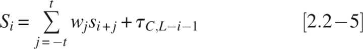where τ_N,k or τ_C,k is a constant tail adjustment value for any residue at a distance, k, from the amino or carboxyl terminus, respectively; L is the sequence length. Tail adjustments, if included, are added to each of the 30 positions at either end of the sequence.

Predictor optimization

Adjustable predictor parameters include disorder propensities (σ), window position weights (w), and N- and C-terminal tail adjustment values (τ). Predictor parameters were optimized with crystallographic data, using a simulated annealing algorithm. Parameter values were perturbed and accepted or rejected in a stepwise manner to maximize a receiver operating characteristic (ROC) score (Gribskov and Robinson 1996), calculated as follows. Disorder scores are calculated for residues (positions) in a set of sequences of proteins with structures. Residues are classified as ordered or disordered based on crystallographic data and are sorted by their predictor-assigned disorder scores. The ROC score is calculated by:

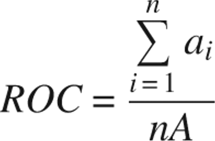where ai is the number of disordered residues that sort by score above the ith ordered residue; A is the total number of disordered residues; and n is a limiting number of ordered residues, calculated in our case as a fraction of the total number of ordered residues. A ROC_0.5 score was used, making n one half the total number of ordered residues. This procedure optimizes the higher specificity half of a ROC curve, potentially reducing the effects of anomalous behavior of low-scoring disordered residues on optimized parameters.

Parameter perturbations were generated according to the following Very Fast Annealing (VFA) function (Cai and Shao 2002):

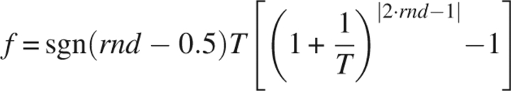where T is perturbation temperature, and rnd is a random number (0 ≤ rnd < 1). f is a fraction (–1 ≤ f < 1). A parameter, u, is perturbed (u′) by

where D is the maximum perturbation quantity. If u′ is too low or too high, it is set to its minimum or maximum value, respectively. Perturbed sets of parameters were accepted or rejected essentially as follows (Metropolis et al. 1953):

• If ΔE ≤ 0 accept

• If ΔE > 0 and

• rnd < exp(–ΔE/T) accept

• otherwise reject

Sequence and profile-based predictors were first optimized without tail adjustments. Disorder propensities were normalized to produce a score distribution that approximates a standard, normal distribution. N-terminal methionine and miscellaneous residue-type disorder parameters were set to 0. Scores may be interpreted as a Z-score (difference in units of standard deviations from the average nonterminal, ordered residue). Normalized disorder propensities were then held constant and tail adjustment values were optimized for the sequence- and profile-based predictors. For the sequence-based predictor with tail adjustments, a separate disorder propensity was optimized for amino-terminal methionine.

Data set

Optimization and testing data include X-ray crystallographic data from domains in 1912 families in the first fivefold classes of the SCOP version 1.67 (Andreeva et al. 2004) (all α, all β, α/β, α + β, and multidomain) (Table 3). Structures dated before 2000 or with a resolution >3.0 Å were excluded. Residues found in SEQRES entries with missing C − α carbon coordinates (or occupancy 0) are considered disordered, while remaining residues are considered ordered. Residues in disordered stretches less than four residues long were excluded. Residues between domains were assigned to a nearby domain. Domains with certain issues (e.g., mismatches between SEQRES sequence and structural sequence, or atom occupancies out of the 0–1 range) were excluded.

In optimizing the disorder propensities for sequence and profile-based predictors, residues at termini (18 from the end of the chain or polyhistidine sequence, if present) were excluded from ROC score calculation to avoid spurious effects from compositional bias at sequence ends (notably for methionine and histidine). Terminal residues were included in the ROC score calculation when optimizing tail adjustment parameters.

Different subsets of the data were periodically selected for measuring parameter performance during optimization. To reduce overrepresentation of certain families or individual structures, a data subset included one protein from each family with more than six representatives; families with five or less representatives were represented in proportion to family size (i.e., one-member families represented ∼1/5 of the time; two-member families ∼2/5 of the time, etc.).

Profiles

The same PSI-BLAST results were used both in developing and testing our profile-based predictors and in testing DISOPRED2. Profiles were built using default values (three iterations, E-value cutoff 0.001). Final alignments included segments from up to 1000 different sequences. Modified COMPASS code (Sadreyev and Grishin 2003) was used to generate final profiles. Use of position-specific independent counts reduced overrepresentation of closely related sequences (Sunyaev et al. 1999). Pseudo-counts (Tatusov et al. 1994) were generated using the BLOSUM62 (Henikoff and Henikoff 1992) matrix. At each position in a profile, the pseudo-count values for the set of all standard residue types were normalized to an exact sum of 1, producing fractional weights that estimate the degree to which each residue-type characterizes that position in the alignment.

Cross validation

To estimate the accuracy of our disorder predictions and to evaluate the consistency of our method, a five-way cross validation was performed. Crystallographic data was split into five subsets. Four out of the five data subsets form a “training set” for optimization of predictor parameters, and the remaining data subset forms a “testing set” for assessment of performance for each of five optimizations. The five sets of optimized parameters were averaged to give final values. Domains were randomly assigned into the five data subsets by SCOP family (see Table 4) so that highly similar sequences could not be shared by concomitant training and testing sets.

Table 4.

Number of SCOP families and individual domains represented in each cross validation data subset

Analysis

Our optimized amino acid residue disorder propensities were compared with several amino acid property scales. ROC curves measure performance for the optimized predictors, for DISOPRED2, and with various indices substituted for optimized disorder parameters in the simple sequence predictor. For each different disorder predictor, ROC curves are calculated for each of the five data subsets (see preceding section on cross validation); then corresponding points from the five resulting ROC curves are averaged to produce final ROC curves. In the case of our optimized predictors, optimized parameters are averaged from the results of five optimization runs using five training sets (see section on cross validation); for each of these optimization runs, a ROC curve is calculated using the corresponding testing data set, which was excluded during optimization. As during optimization, certain residues were excluded from ROC curve calculations and other performance analyses (see Data set section).

Additionally, squared correlation coefficients (R²) were calculated for our disorder propensities and 516 published amino acid property scales found in the AAindex database (Kawashima and Kanehisa 2000), quantifying the degree of covariance between our optimized parameters and each of these scales. Relationships between scales derived from structural data and scales derived from partitioning experiments were examined.

Our optimization-derived disorder propensities were compared with disorder propensities derived statistically (as LORs) using samplings of data from the data sets used for optimization, balanced in an equivalent fashion. LORs behave in a linear fashion and provide a good statistical measure of relative propensity. The disorder versus order LOR for amino acid type i is calculated as follows:

where P(i | diso) denotes the probability of the occurrence of residue type i in the disordered state and P(i | ord) denotes the probability of residue type i in the ordered state. LORs are also calculated in a similar manner for profiles using the profile frequencies of each amino acid type at ordered and disordered positions. LORs were calculated from DisProt (Sickmeier et al. 2007) by considering noted residues as disordered and all other residues as ordered. N-terminal methionines were treated as a separate residue category.

References

- Altschul S.F., Madden, T.L., Schaffer, A.A., Zhang, J., Zhang, Z., Miller, W., and Lipman, D.J. 1997. Gapped BLAST and PSI-BLAST: A new generation of protein database search programs. Nucleic Acids Res. 25: 3389–3402. doi: 10.1093/nar/25.17.3389. [DOI] [PMC free article] [PubMed] [Google Scholar]
- Andreeva A., Howorth, D., Brenner, S.E., Hubbard, T.J., Chothia, C., and Murzin, A.G. 2004. SCOP database in 2004: Refinements integrate structure and sequence family data. Nucleic Acids Res. 32: D226–D229. doi: 10.1093/nar/gkh039. [DOI] [PMC free article] [PubMed] [Google Scholar]
- Bastolla U., Porto, M., Roman, H.E., and Vendruscolo, M. 2005. Principal eigenvector of contact matrices and hydrophobicity profiles in proteins. Proteins 58: 22–30. [DOI] [PubMed] [Google Scholar]
- Butler J.A.V. 1937. The energy and entropy of hydration of organic compounds. Trans. Faraday Soc. 33: 229–236. [Google Scholar]
- Cai W. and Shao, X. 2002. A fast annealing evolutionary algorithm for global optimization. J. Comput. Chem. 23: 427–435. [DOI] [PubMed] [Google Scholar]
- Chandler D. 2005. Interfaces and the driving force of hydrophobic assembly. Nature 437: 640–647. [DOI] [PubMed] [Google Scholar]
- Cheng J., Sweredoski, M.J., and Baldi, P. 2005. Accurate prediction of protein disordered regions by mining protein structure data. Data Mining Knowledge Discovery 11: 213–222. [Google Scholar]
- Chothia C. 1976. The nature of the accessible and buried surfaces in proteins. J. Mol. Biol. 105: 1–12. [DOI] [PubMed] [Google Scholar]
- Chou P.Y. and Fasman, G.D. 1974. Conformational parameters for amino acids in helical, beta-sheet, and random coil regions calculated from proteins. Biochemistry 13: 211–222. [DOI] [PubMed] [Google Scholar]
- Cid H., Bunster, M., Canales, M., and Gazitua, F. 1992. Hydrophobicity and structural classes in proteins. Protein Eng. 5: 373–375. [DOI] [PubMed] [Google Scholar]
- Coeytaux K. and Poupon, A. 2005. Prediction of unfolded segments in a protein sequence based on amino acid composition. Bioinformatics 21: 1891–1900. [DOI] [PubMed] [Google Scholar]
- Creighton T.E. 2002 1993. Proteins: Structures and molecular properties, 2nd ed. W.H. Freeman Company, New York.
- Dosztanyi Z., Csizmok, V., Tompa, P., and Simon, I. 2005a. IUPred: Web server for the prediction of intrinsically unstructured regions of proteins based on estimated energy content. Bioinformatics 21: 3433–3434. [DOI] [PubMed] [Google Scholar]
- Dosztanyi Z., Csizmok, V., Tompa, P., and Simon, I. 2005b. The pairwise energy content estimated from amino acid composition discriminates between folded and intrinsically unstructured proteins. J. Mol. Biol. 347: 827–839. [DOI] [PubMed] [Google Scholar]
- Dosztanyi Z., Sandor, M., Tompa, P., and Simon, I. 2007. Prediction of protein disorder at the domain level. Curr. Protein Pept. Sci. 8: 161–171. [DOI] [PubMed] [Google Scholar]
- Esnouf R.M., Hamer, R., Sussman, J.L., Silman, I., Trudgian, D., Yang, Z.R., and Prilusky, J. 2006. Honing the in silico toolkit for detecting protein disorder. Acta Crystallogr. D Biol. Crystallogr. 62: 1260–1266. [DOI] [PubMed] [Google Scholar]
- Ferron F., Longhi, S., Canard, B., and Karlin, D. 2006. A practical overview of protein disorder prediction methods. Proteins 65: 1–14. [DOI] [PubMed] [Google Scholar]
- Galzitskaya O.V., Garbuzynskiy, S.O., and Lobanov, M.Y. 2006a. FoldUnfold: Web server for the prediction of disordered regions in protein chain. Bioinformatics 22: 2948–2949. [DOI] [PubMed] [Google Scholar]
- Galzitskaya O.V., Garbuzynskiy, S.O., and Lobanov, M.Y. 2006b. Prediction of amyloidogenic and disordered regions in protein chains. PLoS Comput. Biol. 2: e177. doi: 10.1371/journal.pcbi.0020177. [DOI] [PMC free article] [PubMed] [Google Scholar]
- Gribskov M. and Robinson, N.L. 1996. Use of receiver operating characteristic (ROC) analysis to evaluate sequence matching. Comput. Chem. 20: 25–33. [DOI] [PubMed] [Google Scholar]
- Guy H.R. 1985. Amino acid side-chain partition energies and distribution of residues in soluble proteins. Biophys. J. 47: 61–70. [DOI] [PMC free article] [PubMed] [Google Scholar]
- Han P., Zhang, X., Norton, R.S., and Feng, Z.P. 2006. Predicting disordered regions in proteins based on decision trees of reduced amino acid composition. J. Comput. Biol. 13: 1723–1734. [DOI] [PubMed] [Google Scholar]
- Henikoff S. and Henikoff, J.G. 1992. Amino acid substitution matrices from protein blocks. Proc. Natl. Acad. Sci. 89: 10915–10919. [DOI] [PMC free article] [PubMed] [Google Scholar]
- Hirose S., Shimizu, K., Kanai, S., Kuroda, Y., and Noguchi, T. 2007. POODLE-L: A two-level SVM prediction system for reliably predicting long disordered regions. Bioinformatics doi: 10.1093/bioinformatics/btm302. [DOI] [PubMed]
- Hopp T.P. and Woods, K.R. 1981. Prediction of protein antigenic determinants from amino acid sequences. Proc. Natl. Acad. Sci. 78: 3824–3828. [DOI] [PMC free article] [PubMed] [Google Scholar]
- Hopp T.P. and Woods, K.R. 1983. A computer program for predicting protein antigenic determinants. Mol. Immunol. 20: 483–489. [DOI] [PubMed] [Google Scholar]
- Jones D.T. and Ward, J.J. 2003. Prediction of disordered regions in proteins from position specific score matrices. Proteins (Suppl 6) 53: 573–578. [DOI] [PubMed] [Google Scholar]
- Kauzmann W. 1959. Some factors in the interpretation of protein denaturation. Adv. Protein Chem. 14: 1–63. [DOI] [PubMed] [Google Scholar]
- Kawashima S. and Kanehisa, M. 2000. AAindex: Amino acid index database. Nucleic Acids Res. 28: 374. doi: 10.1093/nar/28.1.374. [DOI] [PMC free article] [PubMed] [Google Scholar]
- Kyte J. and Doolittle, R.F. 1982. A simple method for displaying the hydropathic character of a protein. J. Mol. Biol. 157: 105–132. [DOI] [PubMed] [Google Scholar]
- Levitt M. 1976. A simplified representation of protein conformations for rapid simulation of protein folding. J. Mol. Biol. 104: 59–107. [DOI] [PubMed] [Google Scholar]
- Li X., Romero, P., Rani, M., Dunker, A.K., and Obradovic, Z. 1999. Predicting protein disorder for N-, C-, and internal regions. Genome Inform. Ser. Workshop Genome Inform. 10: 30–40. [PubMed] [Google Scholar]
- Li X., Obradovic, Z., Brown, C.J., Garner, E.C., and Dunker, A.K. 2000. Comparing predictors of disordered protein. Genome Inform. Ser. Workshop Genome Inform. 11: 172–184. [PubMed] [Google Scholar]
- Linding R., Jensen, L.J., Diella, F., Bork, P., Gibson, T.J., and Russell, R.B. 2003a. Protein disorder prediction: Implications for structural proteomics. Structure 11: 1453–1459. [DOI] [PubMed] [Google Scholar]
- Linding R., Russell, R.B., Neduva, V., and Gibson, T.J. 2003b. GlobPlot: Exploring protein sequences for globularity and disorder. Nucleic Acids Res. 31: 3701–3708. doi: 10.1093/nar/gkg5. [DOI] [PMC free article] [PubMed] [Google Scholar]
- Lise S. and Jones, D.T. 2005. Sequence patterns associated with disordered regions in proteins. Proteins 58: 144–150. [DOI] [PubMed] [Google Scholar]
- Metropolis N., Rosenbluth, A.W., Rosenbluth, M.N., Teller, A.H., and Teller, E. 1953. Equation of state calculations by fast computing machines. J. Chem. Phys. 21: 1087–1092. [Google Scholar]
- Nishikawa K. and Ooi, T. 1986. Radial locations of amino acid residues in a globular protein: Correlation with the sequence. J. Biochem. 100: 1043–1047. [DOI] [PubMed] [Google Scholar]
- Nozaki Y. and Tanford, C. 1971. The solubility of amino acids and two glycine peptides in aqueous ethanol and dioxane solutions. Establishment of a hydrophobicity scale. J. Biol. Chem. 246: 2211–2217. [PubMed] [Google Scholar]
- Oobatake M. and Ooi, T. 1977. An analysis of non-bonded energy of proteins. J. Theor. Biol. 67: 567–584. [DOI] [PubMed] [Google Scholar]
- Pal D. and Chakrabarti, P. 2000. β-sheet propensity and its correlation with parameters based on conformation. Acta Crystallogr. D Biol. Crystallogr. 56: 589–594. [DOI] [PubMed] [Google Scholar]
- Palau J., Argos, P., and Puigdomenech, P. 1982. Protein secondary structure. Studies on the limits of prediction accuracy. Int. J. Pept. Protein Res. 19: 394–401. [PubMed] [Google Scholar]
- Peng K., Radivojac, P., Vucetic, S., Dunker, A.K., and Obradovic, Z. 2006. Length-dependent prediction of protein intrinsic disorder. BMC Bioinformatics 7: 208. doi: 10.1186/1471-2105-7-208. [DOI] [PMC free article] [PubMed] [Google Scholar]
- Prilusky J., Felder, C.E., Zeev-Ben-Mordehai, T., Rydberg, E.H., Man, O., Beckmann, J.S., Silman, I., and Sussman, J.L. 2005. FoldIndex: A simple tool to predict whether a given protein sequence is intrinsically unfolded. Bioinformatics 21: 3435–3438. [DOI] [PubMed] [Google Scholar]
- Punta M. and Maritan, A. 2003. A knowledge-based scale for amino acid membrane propensity. Proteins 50: 114–121. [DOI] [PubMed] [Google Scholar]
- Radzicka A. and Wolfenden, R. 1988. Comparing the polarities of the amino acids: Side-chain distribution coefficients between the vapor phase, cyclohexane, 1-octanol, and neutral aqueous solution. Biochemistry 27: 1664–1670. [Google Scholar]
- Richardson J.S. 1981. The anatomy and taxonomy of protein structure. Adv. Protein Chem. 34: 167–339. [DOI] [PubMed] [Google Scholar]
- Romero P., Obradovic, Z., Kissinger, C., Villafranca, J.E., and Dunker, A.K. 1997. Identifying disordered regions in proteins from amino acid sequence. Proc. IEEE Int. Conf. Neural Networks 1: 90–95. [Google Scholar]
- Rose G.D., Geselowitz, A.R., Lesser, G.J., Lee, R.H., and Zehfus, M.H. 1985. Hydrophobicity of amino acid residues in globular proteins. Science 229: 834–838. [DOI] [PubMed] [Google Scholar]
- Rose G.D., Fleming, P.J., Banavar, J.R., and Maritan, A. 2006. A backbone-based theory of protein folding. Proc. Natl. Acad. Sci. 103: 16623–16633. [DOI] [PMC free article] [PubMed] [Google Scholar]
- Sadreyev R. and Grishin, N. 2003. COMPASS: A tool for comparison of multiple protein alignments with assessment of statistical significance. J. Mol. Biol. 326: 317–336. [DOI] [PubMed] [Google Scholar]
- Shimizu K., Muraoka, Y., Hirose, S., Tomii, K., and Noguchi, T. 2007. Predicting mostly disordered proteins by using structure-unknown protein data. BMC Bioinformatics 8: 78. doi: 10.1186/1471-2105-8-78. [DOI] [PMC free article] [PubMed] [Google Scholar]
- Sickmeier M., Hamilton, J.A., LeGall, T., Vacic, V., Cortese, M.S., Tantos, A., Szabo, B., Tompa, P., Chen, J., Uversky, V.N., et al. 2007. DisProt: The database of disordered proteins. Nucleic Acids Res. 35: D786–D793. doi: 10.1093/nar/gkl. [DOI] [PMC free article] [PubMed] [Google Scholar]
- Street A.G. and Mayo, S.L. 1999. Intrinsic β-sheet propensities result from van der Waals interactions between side chains and the local backbone. Proc. Natl. Acad. Sci. 96: 9074–9076. [DOI] [PMC free article] [PubMed] [Google Scholar]
- Su C.T., Chen, C.Y., and Ou, Y.Y. 2006. Protein disorder prediction by condensed PSSM considering propensity for order or disorder. BMC Bioinformatics 7: 319. doi: 10.1186/1471-2105-7-319. [DOI] [PMC free article] [PubMed] [Google Scholar]
- Sugase K., Dyson, H.J., and Wright, P.E. 2007. Mechanism of coupled folding and binding of an intrinsically disordered protein. Nature 447: 1021–1025. [DOI] [PubMed] [Google Scholar]
- Sunyaev S.R., Eisenhaber, F., Rodchenkov, I.V., Eisenhaber, B., Tumanyan, V.G., and Kuznetsov, E.N. 1999. PSIC: Profile extraction from sequence alignments with position-specific counts of independent observations. Protein Eng. 12: 387–394. [DOI] [PubMed] [Google Scholar]
- Tatusov R.L., Altschul, S.F., and Koonin, E.V. 1994. Detection of conserved segments in proteins: Iterative scanning of sequence databases with alignment blocks. Proc. Natl. Acad. Sci. 91: 12091–12095. [DOI] [PMC free article] [PubMed] [Google Scholar]
- Tomii K. and Kanehisa, M. 1996. Analysis of amino acid indices and mutation matrices for sequence comparison and structure prediction of proteins. Protein Eng. 9: 27–36. [DOI] [PubMed] [Google Scholar]
- Uversky V.N., Gillespie, J.R., and Fink, A.L. 2000. Why are “natively unfolded” proteins unstructured under physiologic conditions? Proteins 41: 415–427. [DOI] [PubMed] [Google Scholar]
- Vihinen M., Torkkila, E., and Riikonen, P. 1994. Accuracy of protein flexibility predictions. Proteins 19: 141–149. [DOI] [PubMed] [Google Scholar]
- Vucetic S., Brown, C.J., Dunker, A.K., and Obradovic, Z. 2003. Flavors of protein disorder. Proteins 52: 573–584. [DOI] [PubMed] [Google Scholar]
- Vullo A., Bortolami, O., Pollastri, G., and Tosatto, S.C. 2006. Spritz: A server for the prediction of intrinsically disordered regions in protein sequences using kernel machines. Nucleic Acids Res. 34: W164–W168. doi: 10.1093/nar/gkl166. [DOI] [PMC free article] [PubMed] [Google Scholar]
- Wang L. and Donald, B.R. 2006. A data-driven, systematic search algorithm for structure determination of denatured or disordered proteins. Comput. Syst. Bioinformatics Conf. 5: 67–78. [PubMed] [Google Scholar]
- Ward J.J., Sodhi, J.S., McGuffin, L.J., Buxton, B.F., and Jones, D.T. 2004. Prediction and functional analysis of native disorder in proteins from the three kingdoms of life. J. Mol. Biol. 337: 635–645. [DOI] [PubMed] [Google Scholar]
- Waugh D.F. 1954. Protein–protein interactions. Adv. Protein Chem. 9: 325–437. [DOI] [PubMed] [Google Scholar]
- Weathers E.A., Paulaitis, M.E., Woolf, T.B., and Hoh, J.H. 2004. Reduced amino acid alphabet is sufficient to accurately recognize intrinsically disordered protein. FEBS Lett. 576: 348–352. [DOI] [PubMed] [Google Scholar]
- Williams R.M., Obradovic, Z., Mathura, V., Braun, W., Garner, E.C., Young, J., Takayama, S., Brown, C.J., and Dunker, A.K. 2001. The protein non-folding problem: Amino acid determinants of intrinsic order and disorder. Pac. Symp. Biocomput. 6: 89–100. [DOI] [PubMed] [Google Scholar]
- Wimley W.C., Creamer, T.P., and White, S.H. 1996. Solvation energies of amino acid side chains and backbone in a family of host-guest pentapeptides. Biochemistry 35: 5109–5124. [DOI] [PubMed] [Google Scholar]
- Yang Z.R., Thomson, R., McNeil, P., and Esnouf, R.M. 2005. RONN: The bio-basis function neural network technique applied to the detection of natively disordered regions in proteins. Bioinformatics 21: 3369–3376. [DOI] [PubMed] [Google Scholar]
- Zhou H. and Zhou, Y. 2004. Quantifying the effect of burial of amino acid residues on protein stability. Proteins 54: 315–322. [DOI] [PubMed] [Google Scholar]