Population Genetics of Polymorphism and Divergence Under Fluctuating Selection

Abstract

Current methods for detecting fluctuating selection require time series data on genotype frequencies. Here, we propose an alternative approach that makes use of DNA polymorphism data from a sample of individuals collected at a single point in time. Our method uses classical diffusion approximations to model temporal fluctuations in the selection coefficients to find the expected distribution of mutation frequencies in the population. Using the Poisson random-field setting we derive the site-frequency spectrum (SFS) for three different models of fluctuating selection. We find that the general effect of fluctuating selection is to produce a more “U”-shaped site-frequency spectrum with an excess of high-frequency derived mutations at the expense of middle-frequency variants. We present likelihood-ratio tests, comparing the fluctuating selection models to the neutral model using SFS data, and use Monte Carlo simulations to assess their power. We find that we have sufficient power to reject a neutral hypothesis using samples on the order of a few hundred SNPs and a sample size of ∼20 and power to distinguish between selection that varies in time and constant selection for a sample of size 20. We also find that fluctuating selection increases the probability of fixation of selected sites even if, on average, there is no difference in selection among a pair of alleles segregating at the locus. Fluctuating selection will, therefore, lead to an increase in the ratio of divergence to polymorphism similar to that observed under positive directional selection.

TWO mechanisms by which evolution can occur are the adaptive process of natural selection and the neutral processes of genetic drift. Which of these is the principal force in the evolution of a population has been one of the central issues in evolutionary biology. An early exchange in this debate was over the changes in the frequencies of a color polymorphism in a population of the scarlet tiger moth, Callimorpha (Panaxia) dominula. Fisher and Ford (1947) argued that the population size was too large for the changes in the frequencies to be due to drift and suggested that fluctuating selection must be acting. Wright (1948) replied by arguing that multiple factors could affect a population and that the effective population size might be much smaller than the census population size.

The potential importance of fluctuating selection on the rate and patterns of molecular evolution is well established on the basis of theoretical and simulation arguments (see Gillespie 1991, 1994). While it is likely that changing environmental conditions affect the fitness and level of genetic variation in natural populations, only a handful of empirical population genetic studies have sought to investigate the issue. Part of the reason this problem remains understudied is the lack of powerful statistical tools for comparing patterns of polymorphism to the predictions under fluctuating selection.

We begin by summarizing key experimental evidence for the importance of fluctuating selection. Mueller et al. (1985) developed statistical tools on the basis of time series analysis to examine variations in allele frequencies. These tests were applied to Drosophila pseudoobscura and D. persimilis populations sampled over a 3-year period. They found significant evidence that fluctuating natural selection likely maintained genetic polymorphisms in 15–20% of cases, suggested by correlated allele frequencies at different enzyme loci. Their model allowed for time-correlated changes in the environmental conditions and it was noted that the power to detect selection was at a maximum when the environmental changes were strongly positively correlated in time relative to the sampling time. A year later, Lynch (1987) argued that their findings of fluctuating selection effects could have been the result of nearby migration that could cause shifts in gene frequency. To eliminate this possibility, he used enzyme loci in Daphnia populations. These populations were large enough to dismiss significant variation due to drift over the timescale of the study and isolated enough to preclude mass migration. He detected variation in allele frequencies attributable to fluctuating selection in the short term, but also discovered that the time-averaged selection coefficients for all loci were not significantly different from zero.

A decade later, Cook and Jones (1996) reexamined some of the earlier results by Fisher and Ford. Analyzing census data from natural and artificial colonies of C. dominula, they concluded that the color polymorphism was maintained by frequency-dependent selection (i.e., selection for a rare variant and against a common variant). They posited small effective population size as the reason for the large variation in observed frequencies, as opposed to fluctuating selection acting on the populations. More recently, O'Hara (2005) took a Bayesian approach to fit the frequencies of the same medionigra gene in C. dominula examined by Fisher and Ford, with the aim of disentangling the relative contribution from both drift and selection in the observations. He inferred that, apart from a recent 8-year period (from the total 60 years of observations), random drift could explain most of the data, but effects of selection were also present. Furthermore, he determined that the time-averaged selection coefficients were close to zero and no change in fitness over the length of the study could be detected, in agreement with previous authors. In contrast to these earlier works, we develop procedures for estimation of fluctuating selection coefficients from sequence polymorphism data taken from a sample of individuals at a single point in time.

For statistical estimation and the derivation of the theoretical site-frequency spectrum, we follow the Poisson random-field approach (Sawyer and Hartl 1992; Hartl et al. 1994). This framework has proved to be useful in estimating mutation and selection parameters in a variety of population genetic settings including genic selection in a population of constant size (Bustamante et al. 2001), general diploid selection (Williamson et al. 2004), and selection in a population undergoing a change in size (Williamson et al. 2005). In all of the cases examined, the site-frequency spectrum contains sufficient information so as to allow for parameter estimation and hypothesis testing given sufficient polymorphism data (normally in the hundreds or thousands of SNPs).

Our first step is to calculate the predicted effect of fluctuating selection on the site-frequency spectrum (SFS). That is, the SFS is the number of mutations at frequency , where 1 ≤ i < n − 1 and n is the number of individuals sampled. To obtain the SFS we use a diffusion approximation for the stationary distribution of the mutation frequencies in a large population. Kimura (1954) was the first to attempt to use diffusion theory to study how the allele frequencies might change under fluctuating environments. There was an error in the calculation that was later corrected by Gillespie (1973) and Jensen (1973). Karlin and Levikson (1974) studied the model with independent fluctuations in more detail and with some simulations. They calculated fixation probabilities and the expected time to fixation under different assumptions. Takahata et al. (1975) (TIM) derived the diffusion approximation when fluctuations were correlated in time. The TIM model served as a springboard for the rich body of theoretical investigation by Gillespie and others (see Gillespie 1991). Briefly, the TIM model is part of a class of diploid selection models denoted by Gillespie as stochastic additive scale–concave fitness function (SAS–CFF) models. SAS describes the stochastic additive scale to which alleles contribute, and the additive scale is mapped to a CFF that is used to assign fitness to the different genotypes. These models can also be extended to include dominance, subdivision, or autocorrelations in the environment.

To compute the theoretical SFS when there are temporal fluctuations in the environment, we use the diffusion approximation. We take the mean selection coefficient of each allele to be equal, implying a net mean selection coefficient of zero. This is in agreement with the conclusions of earlier works on the absence of a long-term net fitness advantage between alleles, when examining temporal data. We also derive the theoretical site frequency, assuming an autocorrelation in environmental changes. As a validation of the diffusion approximation, we compare the diffusion approximation prediction for the SFS to data gathered from simulation assuming independent sites.

The site-frequency spectrum data are then used to define a maximum-likelihood function from which we obtain estimates of the mutation rate parameter, θ, and a parameter, β, which measures the variance of the fluctuating selection coefficients. This allows the derivation of the asymptotic variance and covariances for these parameters and a comparison to likelihood-based uncertainty bounds. To distinguish between fluctuating selection and a neutral model, we compute the power of the likelihood-ratio test (LRT) for various values of β. We also investigate the coverage of β and explore the power to distinguish fluctuating selection and negative or positive (directional) selection by generating a series of empirical distributions for the LRT statistic under the appropriate null hypothesis.

THEORY AND METHODS

Diffusion approximation for the site-frequency spectrum:

We begin with the model of Karlin and Levikson (1974). Consider two alleles A and a that have the following fitnesses

where σ⁽ⁿ⁾ and τ⁽ⁿ⁾ are identically distributed random variables representing the relative change in fitness due to random environmental changes. We follow their procedure in looking for the diffusion approximation to then calculate the site-frequency spectrum. To derive the diffusion approximation, we first need the drift coefficient and the variance. The drift coefficient is

(1)

and the variance is

(2)

(For a full derivation see the appendix.) To simplify the formulas we let

so that

(3)

At first glance, the drift term looks like balancing selection, but there is an extra term in the variance that speeds up the movement and prevents accumulation of intermediate-frequency alleles. We consider the special case in which σ and τ have the same distribution, so E(σ − τ) = 0, E(σ² − τ²) = 0, and hence α = β/2. In these models, β is a scaled measure of the total variance in the fluctuating selection since var(σ − τ) = β/(2N) . Thus, substituting α = β/2 we get

(4)

Finding the stationary solution to the diffusion equation (see the appendix) and using the formula derived in Kimura (1962) or in Sawyer and Hartl (1992), we find the density of mutations for a unit overall mutation rate is given by f(y, β)dy, where

(5)

Here, , , and

K(β) is · φ(1), where φ(y) is an increasing scale function normalized by φ(0) = 0. To show the relationship to the neutral case (β = 0), we rewrite (5) as

The function h(β, y) → 1 as β → 0 as we would expect. When β ≠ 0, we find that and

Therefore, compared to the neutral model, the occurrence of rare alleles (with y close to 0) is unaffected by the fluctuating environmental effects while the proportion of high-frequency derived alleles (y close to 1) is higher than expected under neutrality. Intermediate-frequency alleles, however, are underrepresented with respect to the neutral case (see results). The reason for this is that fluctuating selection (unlike directional selection) does not result in a net increase in the sojourn time of selected mutations relative to neutrality. Rather, it appears as if the increase in fixation comes at the expense of higher genetic drift at intermediate-frequency alleles.

Autocorrelated selection coefficients:

Takahata et al. (1975) considered a Wright–Fisher diffusion with varying selection:

They let and and found that in the diffusion approximation

To connect this to the model discussed above (which assumed σ and τ uncorrelated in time), suppose that E(σ² − τ²) = 0, let , and equate V = E(σ − τ)²/2. This suggests that to extend the previous analysis to autocorrelated selection coefficients, (σ_n, τ_n), all we do is replace E(σ − τ)²/2 by the sum of the autocovariance function

(6)

if E(σ − τ) = 0. In other words, we use (6) as the formula for β/(4N) in (5). While the above is not a proof, it is supported by the calculations that Takahata et al. (1975) give for their model. We also show numerically that substituting the autocovariance (6) for V gives a good approximation to the case where σ and τ are not independent and identically distributed.

We consider two different forms for the autocorrelation of the selection coefficients. In an earlier article (Gillespie 1993), Gillespie used an autocorrelated model where the fitness of an allele changed by assigning a random fitness 1 + X_i(t). The X_i(t)'s are normal random variables that remain constant, on average, for 1/a generations before changing,

(7)

where ξ(t) are independent and identically distributed normal random variables with mean zero and variance σ². For this case the autocovariance is

and

(8)

We also consider an autocorrelated model with a higher degree of noise every generation:

(9)

The sum of the autocovariance is

(10)

We get this quantity by rewriting the X_i(t)'s as the sequence of random variables X(0), X(0) + S₁, X(0) + S₂ , … , X(0) + S_k−1, ξ_k, where S_k = ξ₁ + ξ₂ + … + ξ_k. To find the covariance we need to find

(11)

The middle terms disappear since X(0) and S_k are independent and since for j > i and S_i, S_j−i are independent. Thus the covariance is

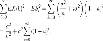(12)

To evaluate the sum in the second line of (12), we can rewrite it as

and now note that the sum (on the right) is the geometric mean so (12) simplifies to

(13)

Again, the quantity (10) is simply substituted for β/(4N) in Equation 5.

Site-frequency spectrum:

Whether we are discussing the time-correlated or -uncorrelated selection model, the stationary polymorphism density of the frequency of a single mutation per unit overall mutation rate is

(14)

Given f(q, β) we can now write formulas for the expected site-frequency spectrum, following Bustamante et al. (2001). For a particular site containing a derived mutation at frequency q in the population, the probability of sampling i sequences with the derived mutation and n − i with the ancestral type is binomially distributed with parameters n and q. We assume an infinite-sites model of mutation where sites are independent, and each mutation that enters the population is described by the two-allele model outlined in the previous section. Therefore, if mutations are entering the population at rate θ/2, the number of sites that have a derived mutation count i, i.e., the site-frequency spectrum, , are independent Poisson-distributed random variables with mean θF(i, β), where

(15)

Simulations:

We verify the accuracy of the diffusion approximation in the previous section, using independent Wright–Fisher Monte Carlo simulations for each site. The numerical routine proceeds as follows:

1. Run Wright–Fisher simulations to estimate the derived mutation frequency, starting at geometrically distributed time intervals measured in generations with rate θ/2. This represents the appearance of a mutation at a previously unmutated site (the sites are independent, so each mutation follows the two-allele model described earlier). The mutant and ancestral alleles have fluctuating selection coefficients, σ and τ, with strengths and autocorrelation parameters dictated by the model we are simulating. The population size for the Wright–Fisher simulations, N, should be sufficiently large such that the diffusion approximation holds. More specifically, the variances of the selection parameters, quantified by β should be of order . Thus β is of order one. We have chosen N = 2000 for all results presented here.

2. After a suitable burn-in to ensure stationarity (10N generations in our simulations), we begin to sample from the population at regularly spaced time intervals. At each time interval, we determine the population frequency of each of the derived mutations. The number of derived mutations in the population (i.e., the number of segregating sites, S) is simply the number of Wright–Fisher trajectories that have not been fixed or lost at the given sample time.

3. For each derived mutation with population frequency p_i, i = 1, … , S, we generate a binomial random variable with parameters n and p_i, which gives the number of derived mutations of that type seen in a sample of size n. (We choose n = 20.)

4. We make a histogram {y₁, y₂, … , y_n−1} of the number of sites carrying derived mutations that occur with frequency 1, … , n − 1 in the sample. This sample provides one realization of the site-frequency spectrum for a given value of β. The results are discussed later and shown in Figure 2.

Figure 2.—

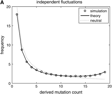
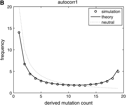
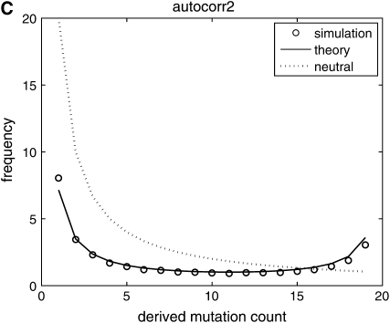
Comparison of predictions from diffusion theory to Monte Carlo simulation with β = 50 and θ = 20. (A) Selection coefficients are drawn independently from generation to generation; (B) selection coefficients have a 90% chance of being identical to the selection coefficient in the previous generation; (C) selection coefficients have a 90% chance of being identical to the selection coefficient in the previous generation plus a random uncorrelated component. In all cases, simulation results are well predicted by theory.

Parameter estimation and inference:

As the site-frequency spectrum is independent Poisson distributed, the likelihood function for an observed spectrum, {y_i}, is given by

(16)

Therefore, the log-likelihood function [dropping the term log(y_i!) independent of parameters] is

(17)

The parameters θ and β can be estimated by maximizing the likelihood (using standard optimization techniques, e.g., conjugate gradient). We note (as in Bustamante et al. 2001) that the maximizer of θ for a given β is easily computed to be , where is the number of segregating sites in the sample. Therefore we can work with the profile log-likelihood function, , which is now a function of a single variable. We use both simulation and asymptotic theory to study properties of these estimates. We follow Bustamante et al. (2001), where all their equations (9)–(32) apply to this method as well, with the appropriate changes given the new expression for f(q, β).

To obtain asymptotic confidence intervals, we must compute the inverse of the Fisher information matrix (FIM), I, given by the expected value of the Hessian of −1 times the log-likelihood function (17):

(18)

The derivatives are all evaluated at the maximum-likelihood estimates (MLEs) for the parameters. As we now show, the mixed partial derivatives are in fact zero for all values of θ and β, so the FIM is diagonal and the covariances Cov(β, θ) = 0. To see this, note that

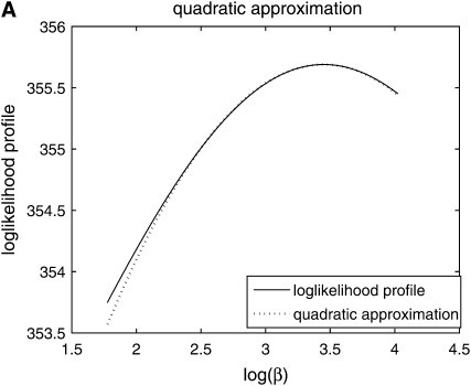
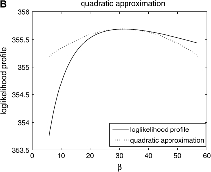
where . In fact, f(y, β) + f(1 − y, β) does not depend on β, which implies that is independent of β; therefore is constant. It is more convenient to work with log β since the profile-likelihood function is better approximated by a Gaussian when using this transformation (Figure 1). By the invariance principle of maximum likelihood, the estimates of the parameter are not affected, but we obtain better performance when far away from the maximum in calculating derived statistics such as confidence intervals. For example, using the log β transformation, we are assured that the lower confidence bounds in the original coordinates are prevented from being negative. The asymptotic variance–covariance matrix for the ML estimates is provided by the inverse FIM,

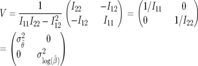(19)

For a 95% confidence interval on , we compute . For the confidence interval is .

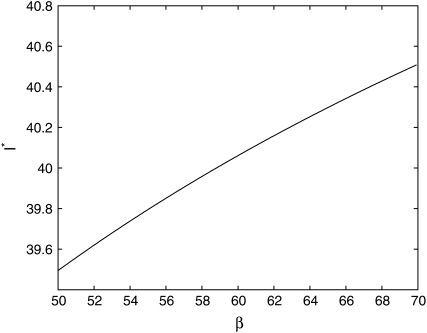
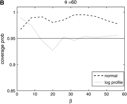
Figure 1.—

Comparison of normal approximation to the log-likelihood function for (A) log β and (B) β.

For the empirical distribution of the parameter estimates, we generate 1200 data sets (site-frequency spectra) for given values of θ and β. We then compute the MLE values and for each of the data sets and obtain 95% confidence intervals on the basis of both a normal approximation of the sampling distribution of the MLE as well as a χ²-approximation of the sampling distribution of the log likelihood.

Unfortunately, the parameters involved in the autocorrelated cases are not individually identifiable; they enter the likelihood expression only through β. That is, for both of the autocorrelated cases we have β = 4Ng(σ², a) where g is the function described in (10) or (8). There is a one-parameter family of pairs of values for σ² and a that yields the same value for β. Note that, for the form of autocorrelation in (7), β = 4Nτ · v (τ = 1/a, and v is the variance of the autocorrelated noise); then, given an MLE for β, , any combination of (τ, v) with τ ≥ 1 and will be consistent with the data.

RESULTS AND DISCUSSION

The site-frequency spectrum:

In the theory and methods section we computed the expected frequency of the derived alleles in the whole population and we can calculate the expected site-frequency spectrum θF(i, β) for a sample of size n. To validate the theory we use simulations (described in the Simulations section) with n = 20, θ = 20, and β = 50. The expected site-frequency spectra are shown in Figure 2. The diffusion approximation is excellent; the data generated by the simulation for the independent case agree with the theory (see Figure 2A). Note that as mentioned before, the more common alleles are favored while alleles with intermediate frequencies are underrepresented, and there are fewer rare alleles than in the neutral case. Another interesting feature is that the expected number of segregating sites does not change with β since (the integrand is an odd function), which implies that is constant. For the autocorrelated case corresponding to (7) and (9) see Figure 2, B and C. We used a = 0.1, which represents a change in the environment about every 10 generations, on average. The theory curve is slightly off at the edges of the spectrum but it is sufficiently accurate as to validate our substitution of E(σ − τ)²/2 by the sum of the autocovariances.

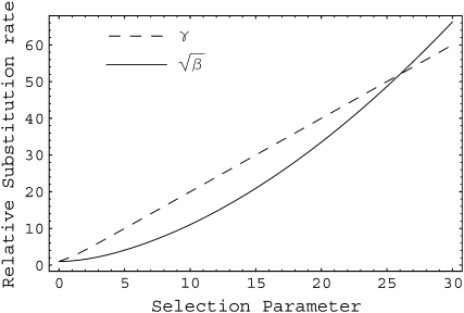
We present in Figure 3 the predicted fixation rates relative to neutrality for fluctuation selection and directional selection as a function of the selection parameter. The natural scaling is for the fluctuating selection model and γ = 2Ns for the directional selection model. We see that in the parameter range of [0, 30], the two models make qualitatively similar predictions as the increase in substitution relative to neutrality. This result suggests that fluctuating selection will lead to an excess of divergence relative to polymorphism and in the analysis of protein-coding DNA sequences result in rejection of the McDonald–Kreitman test in the same direction as positive selection.

Figure 3.—

Fixation rate of mutations under directional selection with scaled selection coefficient γ or under fluctuating selection with standard deviation relative to neutrality (γ = 0).

We also considered the impact of fluctuating selection on commonly used SFS statistics for detecting deviation from the standard neutral model. Surprisingly, we find that the expected values of Tajima's D and Fu and Li's statistics are not affected by fluctuating selection. A potential explanation for this observation is that Tajima's D is derived from the folded site-frequency spectrum that is not nearly as affected by selection as the unfolded SFS that can distinguish rare from high-frequency derived alleles.

The power of the test:

We perform a test of neutrality that compares the null hypothesis (β = 0) with the alternative hypothesis (β ≠ 0). The likelihood test statistic is

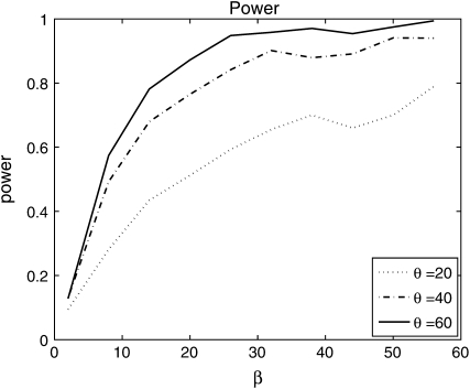
where is Watterson's (1975) estimator of θ and 2 ln(Λ) has (asymptotically) a χ²-distribution with 1 d.f. To assess the power of the test, we generate 1200 data sets (described in the Simulations section), and for each data set, we apply the LRT at the (1 − α) significance level where α = 0.05. We used different levels of mutation θ ∈ {20, 40, 60} with β ∈ {2, 8, 14, 20, 26, 32, 38, 44, 50, 56}. The results are shown in Figure 4. We observe that the test has very good power to detect deviations from neutrality as θ and β increase. For higher mutation rates, there are a larger number of sites with derived mutations in any given sample, and intuitively the power to detect for selection is improved. The P-values obtained here depend on the independent-sites assumption. However, it is possible to find P-values in the presence of linkage by using coalescent simulations with recombination to find the critical value for the test statistic (Zhu and Bustamante 2005).

Figure 4.—

Power of the LRT test. On the x-axis are the different values of β under which the data were simulated. The y-axis represents the proportion of data sets of 1200 that rejected neutrality (β = 0).

Sampling distributions of and :

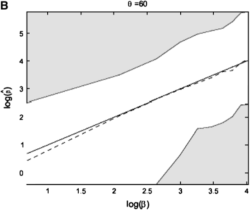
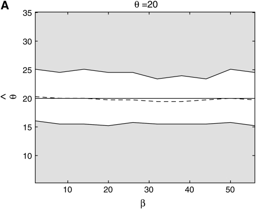
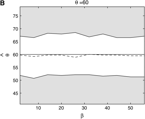
Using the generated data under different mutation rates we find that the distributions for are centered around the true value (Figure 5) with increasing variance as β moves away from zero. The variance is large for smaller θ. This happens because for some data sets we get very large values for and can have . For example, if we use a data set generated with θ = 20 and β = 56, we get β = ∞. If one plots the log-profile-likelihood function, it is easy to see that the function is monotonic and peaks at β = ∞ (see Figure 6). On the other hand, the estimation of θ is excellent for the different values of β. The variance stays mostly constant as we vary β (see Figure 7).

Figure 5.—

The sampling distributions of log β as a function of β for two values of the mutation rate (θ ∈ {20, 60}). The dashed lines connect the median estimates across values of β. The open space contains 95% of the observed values for .

Figure 6.—

The log-profile-likelihood function of β for a data set with true β = 56 and maximum-likelihood estimate at β = ∞.

Figure 7.—

The sampling distributions of θ as a function of β for two values of the mutation rate (θ ∈ {20, 60}). The solid horizontal line is the true value of θ and the dotted line is the median of . The open space contains 95% of the observed .

Confidence sets:

We examined two types of confidence sets: (1) the region that contains (1 − α)100% of the area under the normal approximation to likelihood function and (2) the region in the profile-likelihood space that is likelihood units from the maximum-likelihood point. The corresponding area at α = 0.05 is 1.96 standard deviations away from , where the standard deviation is given by for the first confidence set. For the second confidence set, at α = 0.05, this corresponds to the region where likelihood units.

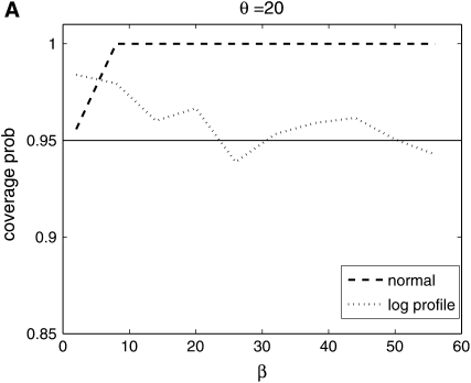
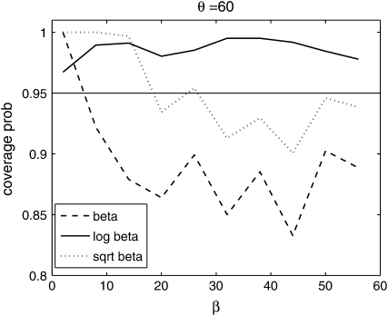
From Figure 8, we see that the confidence intervals based on the profile-likelihood function have good coverage. The confidence intervals based on the normal approximation to the likelihood do cover very well for all values of β, in fact, extremely well for θ = 20. This occurs because for smaller θ it is common to see that the best estimate for β is zero. Since f(i, β) is not defined for β = 0, we have to use the limit as β goes to zero. This results in an upper confidence interval that is ∞ and a lower confidence interval that is zero. Here we are estimating log(β) instead of β because the quadratic approximation to the log-profile function is better when we use log(β). It is important to note that sometimes using β does not give good coverage. In Figure 9 we compare the coverage using β, log(β), and β gives bad coverage, gives good coverage, and using log(β) gives big coverage. This implies that perhaps is the best function of β of the three.

Figure 8.—

Coverage of 95% confidence intervals using two different methods for building confidence sets. One is based on the normal approximation and the other uses the difference in profile log likelihood. The coverage under the normal approximation is always higher than when using the profile log-likelihood function.

Figure 9.—

Coverage of 95% confidence intervals under θ = 60 using the normal approximation method for β, log β, and .

Distinguishing between positive selection and fluctuating selection:

We also investigated how much power we have to distinguish fluctuating selection from positive or negative (constant) selection. Since these two models are not nested, we need to empirically find the distribution of our statistic under the null (constant selection) model. That is:

1. Generate a data set as explained in the Simulations section but under the γ-model; i.e., the ancestral allele has fitness one, and the derived allele has fitness 1 + s, where s is constant in time, and γ = 2Ns.

2. Find the MLE estimate of γ using the likelihood for the γ-model [this requires using the appropriate f(y, γ) that is given in Bustamante et al. 2001] and the MLE estimate of β using the likelihood for the β-model.

3. Let .

4. Repeat steps 1–3 M times to generate the empirical distribution of the statistic Λ.

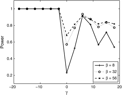
To compute the power to distinguish these two models, we generated data under the β-model and computed the MLE estimates for γ and for β. We then calculated , and we computed Λ_obs for 1000 data sets. The power is then the proportion of times (of 1000) that the P-value was <0.05. This translates to the number of times that Λ_obs lies in the upper 5th percentile of the empirical distribution. Figure 10 shows the results. The power to distinguish fluctuating selection from negative selection is excellent for all values of β. However, the power to distinguish positive selection from fluctuating selection is not very good for small β and the power fluctuations are big; but for bigger values of β the power is satisfactory.

Figure 10.—

Power to distinguish positive and negative selection from fluctuating selection. Data were simulated for β ∈ {8, 32, 56}, n = 20, and θ = 60. The x-axis is the selection coefficient, the parameter of the data where the empirical distribution of the test statistic was obtained to get a critical value for the test.

Conclusions:

Fluctuating selection is potentially an important force in shaping polymorphism, and even though it has received much theoretical attention, it is commonplace to use population genetic models that assume that all new mutations are under constant selection (deleterious, neutral, or positive). We have developed a statistical inference for fitting population genetic models that incorporate temporal fluctuations in the environment. Our simulation results suggest that the method has reasonable power to distinguish fluctuating selection from neutral evolution, with increasing power as the number of segregating sites increases. We also examined the possibility of distinguishing constant selection from fluctuating selection. The power to do so was very good when we tried to distinguish negative selection from fluctuating selection; however, when we looked at positive selection vs. fluctuating selection, it became harder to detect true fluctuating selection when β is small since both models lead to an increase in high-frequency derived alleles.

We also note that fluctuating selection, much like positive directional selection, leads to an increase in the ratio of divergence to polymorphism as compared to neutrality. The magnitude of this effect is very comparable for (standard deviation of fluctuations) and γ (strength of directional selection) in the range of selection parameters likely to be important in molecular evolution. This implies that often-used tests of neutrality that make use of polymorphism and divergence (such as the HKA and McDonald–Kreitman tests) may reject neutrality if fluctuating selection has shaped the evolution of the molecule and the rejection will occur “in the same direction” as for positive selection. This raises the tantalizing hypothesis that the signature of positive selection in Drosophila may really be the result of fluctuating (and not directional) selection. This hypothesis has also recently been put forth in a similar analysis by Mustonen and Lassig (2007).

This method also allowed us to make point estimates for and to compute confidence intervals for these parameters. Finally, we compared methods for making confidence bounds on our estimators. We showed that we obtained good coverage when using the likelihood function directly, but the normal approximation implied by using the Fisher information matrix was often overly conservative.

The approaches outlined here are also readily generalized to more complicated demographic models such as selection in a population undergoing size change (e.g., expansion, contraction, or bottlenecks) (Williamson et al. 2005). Even though this analysis does not incorporate important factors such as population structure and assumes high levels of recombination, this method appears to have good promise for detecting temporal fluctuations in selection from genomewide patterns of polymorphism.

APPENDIX

To derive the diffusion approximation, note that the change in frequency in one generation is

Writing x = we have

Taking the expected value and speeding up time by a factor of 2N the drift coefficient is

(A1)

To compute the variance, let ΔX be the change in frequency and Y be the environment:

To evaluate the first term, recall that the variance of Binomial(2N, p) is 2Np(1 − p) so

since σ and τ are small. As we computed above

This time we can ignore the contribution from the denominator:

Adding the two results and speeding up time by a factor of 2N gives

(A2)

To simplify formulas we let

so that

(A3)

To compute the natural scale we want to solve ψ′(x) = −2b(x)ψ(x)/a(x). To do this, we begin by noting

(A4)

The quadratic in the denominator has two roots r₁ < 0 < 1 < r₂ given by

To evaluate the integral we write

The quadratic in the denominator has two roots r₁ < 0 < 1 < r₂ given by

Note that the two roots are symmetric about .

To find the constants we solve −C + D = 2 and Cr₂ − Dr₁ = −2α/β to find

Integrating

yields

Consider now the special case in which σ and τ have the same distribution so E(σ − τ) = 0, E(σ² − τ²) = 0, and hence α = β/2. Then

and we have the very nice formula

One can check this by noting that

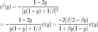when α = β/2 and comparing with (A4). Karlin and Levikson (1974) find ψ(y) = [1 + βy(1 − y)]⁻¹ in their p. 402, but this agrees with our computation since the solution of ψ′(y) = −2b(y)ψ(y)/a(y) is determined only up to a constant multiple. To make it easier to compare with their formulas, we let

(A5)

To compute the natural scale φ, we integrate to find

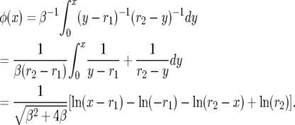(A6)

This is close to but not exactly the same as that in Karlin and Levikson (1974). Their roots are λ₂ = r₁ and λ₁ = r₂, and they write w = β/2, so their constant has 2β instead of 4β.

Since φ(0) = 0, the probability of fixation starting from frequency x is

since and we can write the above as

This is (8) in Jensen (1973). As β → ∞, r₁ → 0, and r₂ → 1 so .

The speed measure

is exactly the same as for the neutral case. Since φ(0) = 0, Green's function G(x, y) is

The expected time to fixation is

Since 1/(1 − y)y = 1/(1 − y) + 1/y has antiderivative log(y/(1 − y)), integrating by parts gives

Since φ(1) − φ(y) ∼ φ′(1)(1 − y) as y → 1 and x log x → 0 as x → 0, evaluating the first term at 1 gives 0, as does evaluating the third term at 0. Evaluating the first term at x cancels with evaluating the third at x, so the above becomes

ψ(y) is symmetric about and log(y/(1 − y)) is antisymmetric about so the first integral vanishes and

When and hence the log is nonnegative throughout the range of integration, so E_xτ is a decreasing function of β. When we can use the fact that the total integral is 0 to write

and we again conclude that this decreases as β increases. This result, which is on p. 402 of Karlin and Levikson (1974), is somewhat surprising since (A3) shows that the diffusion has a drift toward , which will encourage it to spend more time at intermediate values. However, as the computations above show, this effect is counteracted by the increase in a(x).

By Hartl and Sawyer's formula the site-frequency spectrum is

which up to a constant is

References

- Bustamante, C. D., J. Wakeley, G. Sawyer and D. L. Hartl, 2001. Directional selection and the site-frequency spectrum. Genetics 159: 1779–1788. [DOI] [PMC free article] [PubMed] [Google Scholar]
- Cook, L. M., and D. A. Jones, 1996. The medionigra gene in the moth panaxia dominula: the case for selection. Philos. Trans. R. Soc. Lond. B 351: 1623–1634. [Google Scholar]
- Fisher, R. A., and E. B. Ford, 1947. The spread of a gene in natural conditions in a colony of the moth Panaxia dominula. Heredity 1: 143–174. [Google Scholar]
- Gillespie, J. H., 1973. Natural selection with varying selection coefficients-a haploid model. Genet. Res. 21: 115–120. [Google Scholar]
- Gillespie, J. H., 1991. The Causes of Molecular Evolution. Oxford University Press, New York.
- Gillespie, J. H., 1993. Substitution processes in molecular evolution. I. Uniform and clustered substitutions in a haploid model. Genetics 134: 971–981. [DOI] [PMC free article] [PubMed] [Google Scholar]
- Gillespie, J. H., 1994. Substitution processes in molecular evolution. II. exchangeble models from population genetics. Evolution 48: 1101–1113. [DOI] [PubMed] [Google Scholar]
- Hartl, D. L., E. N. Moriyama and S. A. Sawyer, 1994. Selection intensity for codon bias. Genetics 138: 227–234. [DOI] [PMC free article] [PubMed] [Google Scholar]
- Jensen, L., 1973. Random selective advantage of genes and their probabilities of fixation. Genet. Res. 21: 215–219. [DOI] [PubMed] [Google Scholar]
- Karlin, S., and B. Levikson, 1974. Temporal fluctutations in selection intensities: case of small population size. Theor. Popul. Biol. 6: 383–412. [DOI] [PubMed] [Google Scholar]
- Kimura, M., 1954. Process leading to quasi-fixation of genes in a population. Genetics 39: 280–295. [DOI] [PMC free article] [PubMed] [Google Scholar]
- Kimura, M., 1962. On the probability of fixation of mutant genes in a population. Genetics 47: 713–719. [DOI] [PMC free article] [PubMed] [Google Scholar]
- Lynch, M., 1987. The consequences of fluctuating selection for isozyme polymorphisms in daphnia. Genetics 115: 657–669. [DOI] [PMC free article] [PubMed] [Google Scholar]
- Mueller, L. D., L. G. Barr and F. J. Ayala, 1985. Natural selection vs. random drift: evidence from temporal variation in allele frequencies in nature. Genetics 111: 517–554. [DOI] [PMC free article] [PubMed] [Google Scholar]
- Mustonen, V., and M. Lassig, 2007. Adaptations to fluctuating selection in Drosophila. Proc. Natl. Acad. Sci. USA 104: 2277–2282. [DOI] [PMC free article] [PubMed] [Google Scholar]
- O'Hara, R. B., 2005. Comparing the effects of genetic drift and fluctuating selection on genotype frequency changes in the scarlet tiger moth. Proc. R. Soc. Lond. Ser. B 272: 211–217. [DOI] [PMC free article] [PubMed] [Google Scholar]
- Sawyer, S. A., and D. L. Hartl, 1992. Population genetics of polymorphism and divergence. Genetics 132: 1161–1176. [DOI] [PMC free article] [PubMed] [Google Scholar]
- Takahata, N., K. Ishii and H. Matsuda, 1975. Effect of temporal fluctuation of selection coefficient on gene frequency in a population. Proc. Natl. Acad. Sci. USA 72: 4541–4545. [DOI] [PMC free article] [PubMed] [Google Scholar]
- Watterson, G. A., 1975. On the number of segregating sites in genetical models without recombination. Theor. Popul. Biol. 7: 256–276. [DOI] [PubMed] [Google Scholar]
- Williamson, S. H., A. Fledel-Alon and C. D. Bustamante, 2004. Population genetics of polymorphism and divergence for diploid selection models with arbitrary dominance. Genetics 168: 463–475. [DOI] [PMC free article] [PubMed] [Google Scholar]
- Williamson, S. H., R. Hernandez, A. Fledel-Alon, L. Zhu, R. Nielsen et al., 2005. Simultaneous inference of selection and population growth from patterns of variation in the human genome. Proc. Natl. Acad. Sci. USA 102(22): 7882–7887. [DOI] [PMC free article] [PubMed] [Google Scholar]
- Wright, S., 1948. On the roles of directed and random changes in gene frequency in the genetics of populations. Evolution 2: 279–294. [DOI] [PubMed] [Google Scholar]
- Zhu, L., and C. D. Bustamante, 2005. A composite-likelihood approach for detecting directional selection from DNA sequence data. Genetics 170: 1411–1421. [DOI] [PMC free article] [PubMed] [Google Scholar]