An Accurate Model for Genetic Hitchhiking

Abstract

We suggest a simple deterministic approximation for the growth of the favored-allele frequency during a selective sweep. Using this approximation we introduce an accurate model for genetic hitchhiking. Only when Ns < 10 (N is the population size and s denotes the selection coefficient) are discrepancies between our approximation and direct numerical simulations of a Moran model notable. Our model describes the gene genealogies of a contiguous segment of neutral loci close to the selected one, and it does not assume that the selective sweep happens instantaneously. This enables us to compute SNP distributions on the neutral segment without bias.

GENE genealogies under neutral evolution are commonly described by the so-called coalescent process (Kingman 1982; Hudson 1983, 1990, 2002; Nordborg 2001), incorporating recombination and geographical and demographical structure. An important question is how gene genealogies are modified by deviations from neutrality due to positive selection. The answer to this question would help in understanding to what extent and in which way selection has shaped the empirically observed patterns of genetic variation.

Many authors have addressed this question by considering the effect of positive directional selection at a given locus on the gene history at a neighboring neutral locus, arising from the introduction of a new selectively favorable allele in the population. The dynamics of the positive selection itself have been modeled in different ways. Most commonly, a deterministic model of the dynamics of the favored-allele frequency has been adopted (Stephan et al. 1992; Braverman et al. 1995; Kim and Stephan 2002; Przeworski 2002), a notable exception being the early work of Kaplan et al. (1989). Any deterministic model is of course an approximation to a more appropriate model, such as Moran or Wright–Fisher models of directional selection, where the allele frequencies fluctuate randomly in time. The reasons for attempting to ignore these fluctuations are practical ones: the exact simulations are very time consuming (Kaplan et al. 1989), and, in addition, deterministic models are much more amenable to theoretical analysis than the stochastic models.

Several authors have investigated stochastic different equation (SDE) approximations of Wright–Fisher and Moran models for positive selection (Slatkin 2001; Coop and Griffiths 2004; Innan and Kim 2004; Etheridge et al. 2006). These models give a very accurate representation of the spread and fixation of the advantageous allele during the selective sweep. In contrast to the exact simulations, the SDE models can be efficiently simulated (Coop and Griffiths 2004; Innan and Kim 2004), but remain difficult to analyze.

Recently, Durrett and Schweinsberg (2004) discovered an elegant asymptotic model [referred to as the Durrett–Schweinsberg (DS) algorithm in the following] for the genealogy of a single neutral locus during a selective sweep occurring in its vicinity. As the population size N tends to infinity, their coalescent process approximates the Moran model (Moran 1958) with recombination and positive selection. Durrett and Schweinsberg (2004) have argued that the fluctuations of the favored-allele frequency during a selective sweep may have a significant effect on the gene genealogy of a neighboring neutral locus and hence on the distribution of single-nucleotide polymorphisms (SNPs) at that locus. In a range of parameters determined by Durrett and Schweinsberg (2004), the DS algorithm describes the effect of a selective sweep on the gene genealogy of a neutral locus nearby very accurately, in close agreement with numerical simulations of a Moran model.

In this article we suggest a deterministic model for the spread of the favorable allelic type in the population, which is equally accurate as the DS algorithm for the parameters considered in Durrett and Schweinsberg (2004), as shown in Figure 8. For practical purposes, our algorithm has a number of advantages. First, it allows for SNPs to occur during the selective sweep because we do not assume that the sweep happens instantaneously as does the paint-box construction (Schweinsberg and Durrett 2005). This avoids a bias in the patterns of genetic variation at the neutral loci when the number of lines in the sweep is not untypically small. Second, in practical applications, the question usually is how selection affects genetic variation in a contiguous stretch of neutral loci, whereas the DS algorithm describes the gene genealogy of a single locus. Our algorithm, by contrast, determines the ancestral recombination graph of an entire segment of neutral loci close to a selected one. Third, our new algorithm gives an accurate description of selective sweeps in a much wider parameter range than the algorithm proposed by Durrett and Schweinsberg (2004). These properties together make our model suitable for use with the method of Coop and Griffiths (2004) for determining log-likelihood surfaces for the parameters s and N in the Moran model of directional selection, where an accurate and computationally efficient model of the selective sweep is required.

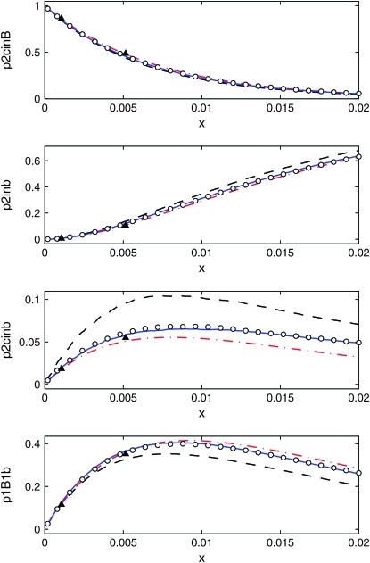
Figure 8.—

The distribution over the partitions as a function of the genetic distance x from the selected locus, from 10,000 samples. We show one section for each of the four partitions. The population size is N = 10⁴, and the selection parameter s = 0.1. The data shown are Moran simulations (circles), the logistic model (dashed black line), our own model (solid blue line), the DS algorithm (dash-dotted red line), and coalescent simulations of Durrett and Schweinsberg (2004) (triangles).

On the theoretical side, we propose an efficient and accurate method for averaging over the fluctuations of the favored-allele frequency. Our scheme gives rise to a deterministic approximation to the time dependence of the favored-allele frequency during the sweep, which, however, is very different from the commonly used logistic model. Our model is as easily implemented as the logistic model, but much more accurate: it gives a very good description of the genealogy of contiguous stretch close to a selected locus provided Ns > 10, where s parameterizes the selective advantage of the favored allele. By contrast, the DS algorithm (Schweinsberg and Durrett 2005) requires in order to be accurate, where r is the recombination rate per individual per generation between the selected and the neutral locus. The logistic model requires very strong selection and large population size (see Figures 8–10).

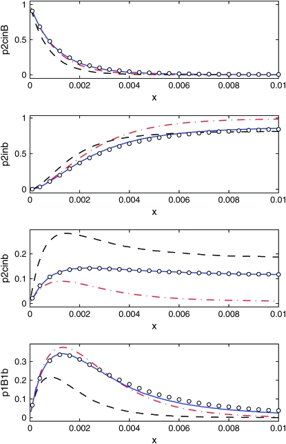
Figure 9.—

As shown in Figure 8, but for s = 0.03.

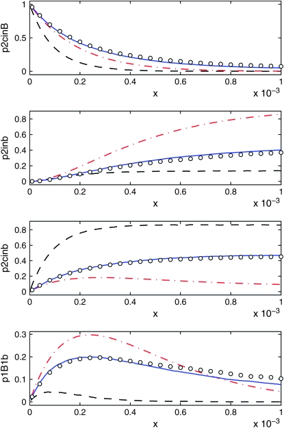
Figure 10.—

As shown in Figure 8, but for s = 0.001.

The remainder of this article is organized as follows. In positive selection and genetic hitchhiking, we give a brief account of previous models of selective sweeps and their influence on the genealogies of nearby loci (usually referred to as “genetic hitchhiking,” see below). In the moran model of positive selection, we describe our implementation of the Moran model. As in Durrett and Schweinsberg (2004) we employ Moran-model simulations as a benchmark for our new algorithm. This new algorithm rests on two parts: a deterministic model for the favored-allele frequency during the sweep (described in averaging over realizations of the sweep) and the coalescent process for a contiguous segment of neutral loci on the same chromosome as the selected locus (described in the background coalescent for neutral loci in the vicinity of a selected one). In results and discussion, we summarize and conclude our results.

POSITIVE SELECTION AND GENETIC HITCHHIKING

Positive selection:

Consider the genetic composition at a certain locus in a diploid population with a constant generation size N. Suppose all 2N gene copies were of the same form b when a new allele B appeared due to a beneficial mutation. Let the new allele B have a fitness advantage (parameterized by s) as compared to the wild-type allele b. The frequency x(t) of allele B at time t is a stochastic process that exhibits a tendency to grow, but that may also become fixed at x = 0 (due to genetic drift) corresponding to the extinction of allele B. Once x(t) has grown sufficiently from the initial low value x(0) = 1/2N, the probability of reaching x = 1 is high; eventually B takes over the population. This process is usually referred to as a “selective sweep.” In the limit of infinite population size, a selective sweep is well approximated by the deterministic model

(1)

see Durrett and Schweinsberg (2004) and the references cited therein. Equation 1 is called the “logistic-growth equation.”

This growth model is a deterministic approximation to the stochastic growth of x(t). The latter is usually modeled in terms of the Wright–Fisher model (Fisher 1930; Wright 1931) with directional selection. This is a haploid population model with nonoverlapping generations where reproduction is described by a biased sampling procedure with replacement: chromosomes are sampled randomly, with replacement, from the previous generation, such that the ratio of the probabilities of choosing a chromosome with the favored allele to that without the favored allele is 1:(1 − s). Direct numerical simulations of the Wright–Fisher model are commonly employed to determine strengths and weaknesses of deterministic approximations such as Equation 1.

In the following we do not employ the Wright–Fisher model as a reference, but a closely related model with overlapping generations introduced by Moran (1958). As shown by Etheridge et al. (2006) it approximates the Wright–Fisher model when the population size is large.

Genetic hitchhiking:

Consider the genetic variation at a neutral locus on the same chromosome as the selected locus. Clearly, the pattern of genetic variation at the neutral locus is influenced by a selective sweep in its vicinity—the smaller the distance is, the larger the influence. When the B allele first appears in the population because of a favorable mutation, the corresponding alleles at the neutral locus have more offspring compared with other alleles not associated with the B allele on the selected locus. Thus, the favored alleles at the neutral locus are spread through the population to a larger extent than can be explained in a neutral model. This effect is known as genetic hitchhiking (Maynard Smith and Haigh 1974). Far from the selected locus, recombination will effectively eliminate linkage between the neutral and the selected loci, so that the influence of the selective sweep becomes negligible.

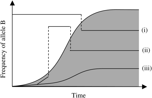
Figure 1 illustrates the hitchhiking effect in terms of the ancestral graph for a small hypothetical sample of sequences taken at a neutral locus. (For the sake of clarity we assume that the selected locus is located left of the neutral locus of interest.) Most ancestral lines can be traced back to the originator of the sweep, but some lines exhibit recombination events allowing them to escape from the subpopulation with the B allele.

Figure 1.—

Illustration of the hitchhiking effect on the ancestral lines of a neutral locus. The shaded area corresponds to individuals with the advantageous allele B at the selected locus in the population. Close to the selected locus, most lines are identical by descent to the originator of the sweep (line iii). Recombination (shown as dashed lines) can cause a line to escape the sweep; i.e., the originator does not belong to the ancestral line, because at some stage a recombination event causes the allele at the neutral locus to be inherited from an ancestral line that has not yet been caught by the sweep (line i). Much less likely, but still possible, is for the line to first escape but later recombine back into the path of the sweep (line ii) (after Durrett and Schweinsberg 2004).

It is straightforward but cumbersome to directly simulate the Wright–Fisher (or Moran) model to analyze how patterns of genetic variation are affected by hitchhiking. Several authors have therefore studied approximations to the growth process of the selected allele frequency x(t). Kaplan et al. (1989) divide the selective sweep into three phases: the early phase is modeled by a supercritical branching process, the middle phase is described by the deterministic logistic growth, and the final phase is viewed as a subcritical branching process. The probability that the sweep succeeds is approximately given by the selective advantage s, when s is small. As a consequence, one may need to iterate this procedure many times to collect enough successful simulations.

This approach has been simplified by ignoring the initial and final (stochastic) phases (see, e.g., Stephan et al. 1992; Braverman et al. 1995; Kim and Stephan 2002; Przeworski 2002) and instead using the deterministic logistic model (1) for the whole sweep. This makes it possible to simulate the sweep backward in time, which in turn enables one to perform computations conditional on that the sweep succeeds. This approach is significantly faster than an algorithm based on the better approximation by Kaplan et al. (1989).

Barton (1998) (see also Otto and Barton 1997) considered a stochastic shift between the introduction of the favored allele and the onset of the deterministic growth; the distribution of the shift is derived from modeling the spread of the beneficial allele in the initial phase of the sweep as a supercritical branching process. The main difference to the logistic model is that the initial growth rate of the frequency of the favorable allele is increased by a factor of one over the probability of the sweep succeeding in the unconditioned model. This approximation captures some of the effects of the conditioning on the success of the sweep and the stochastic growth in the early stages of the sweep. The middle and late stages of the sweep are treated in the logistic approximation. Within his model, Barton gives analytical expressions for the probability that two copies of a neutral marker are identical by descent, assuming that any recombination event leads to ancestral lines escaping the sweep. A similar model was studied by Kim and Nielsen (2004), where the initial phase is ignored and instead the initial frequency of the favorable allelic type is increased by one over the unconditioned probability of fixation.

As argued by Durrett and Schweinsberg (2004), the disadvantage of ignoring the fluctuations is that the probabilities of how lines merge and recombine are not correctly described. They consider the gene genealogy of a selected locus and a nearby neutral locus and propose an elegant approximation to the Moran dynamics, valid in the limit of large population size and strong selection, which captures the stochastic aspects of the sweep and correctly models the partitioning of the neutral lines as a consequence of the selective sweep.

THE MORAN MODEL OF POSITIVE SELECTION

In this section we describe the Moran model (Moran 1958) for the evolution of a diploid population of N individuals. The Moran model is used as a benchmark to test the accuracy of our coalescent model described below in averaging over realizations of the sweep and in the background coalescent for neutral loci in the vicinity of a selected one.

We consider a chromosome with a locus subject to positive selection and determine the evolution of this selected locus, as well as genealogies of neutral loci in its vicinity. In Spread of the advantageous allele during the sweep we describe the growth of the favored-allele frequency in the population. In Conditioning on the fixation of allele B we explain how to condition this process on the success of the selective sweep. This is necessary because in trying to deduce the effect of a sweep on neutral loci nearby we assume that the sweep actually took place. In Gene genealogies of the neutral loci during the sweep we summarize how gene genealogies of such neutral loci are calculated within the Moran model.

Spread of the advantageous allele during the sweep:

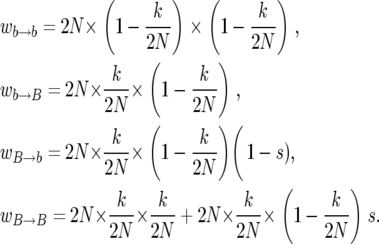
As in the previous section we assume that there is a favored allele at the selected locus, B say, and a set of selectively equivalent variants (unfavorable relative to B), which we refer to collectively as b. The lifetime of each individual is taken to be an independent exponentially distributed variable with expected value of one generation. When an individual dies, it is replaced with a copy of an individual chosen with replacement with uniform probability from the whole population, except that replacement of an individual with the B allele with an individual with the b allele is rejected with probability s; this is what constitutes selection in this model. Instead, a parent is chosen with uniform probability from the set of individuals with the B allele. Thus, s = 0 corresponds to neutral evolution and s = 1 is the strongest possible selection. In short, the population evolves according to a time-continuous Markov process where the different events occur with rates

(2)

The three factors in the rates , where α and β stand for either b or B, have the following interpretations: the first factor is the total rate of replacement events in the population per generation; the second factor is the probability that the line that dies has the allelic type α; the final factor is the probability that the replacing line has the allelic type β. The second term in the rate corresponds to the rejected B-to-b replacements. It follows from Equation 2 that the sum of events is 2N per generation for all values of s.

Durrett and Schweinsberg (2004) use a slightly different version of the Moran model with positive selection. In their model, the rejected B-to-b transitions are ignored, whereas we take them to be B-to-B transitions. This difference does not affect the trajectory of the number of copies of the advantageous allelic type. Yet other versions are conceivable: the corresponding modifications of Equation 2 would require minor changes to the background coalescent described in the background coalescent for neutral loci in the vicinity of a selected one, but we do not discuss these here.

Conditioning on the fixation of allele B:

In each replacement, the number of copies k of allele B in the population is increased by one (corresponding to a event), decreased by one (corresponding to a event), or left unchanged (corresponding to a or a event). Consider the number k_i of copies of the advantageous allelic type in the population after the ith change in k. The sequence k₁, k₂, … , then follows a Markov chain, where the probability that k is increased by one after a replacement where k changes is

(3)

The probability h_k of fixation of the B allele in the population, given that there are k copies at present, equals the probability of fixation after a change in k. With the probability that k increases in (3), one obtains the recursion

(4)

where k is between 1 and 2N − 1. If k is zero, there are no copies of B that can reproduce; hence, h₀ = 0. Similarly, when k = 2N all individuals in the population have the B allele, corresponding to h_2N = 1. With these two conditions the recursion has a unique solution, given by

(5)

(see, e.g., Durrett 2002 and references therein). Usually, the population size is large and the selection parameter is small. If in addition 2Ns is large, we obtain the well-known result that the probability h₁ that the sweep succeeds from a single copy of the B allele is approximately s. This means that if the sweep is initiated with a single copy of the B allele, and the rates are given by (2), in most cases the B allele will become extinct in a few generations because of the fluctuations in the early stage of the sweep. When k reaches a critical level (where ks is relatively large), the probability that the fluctuations will cause B to become extinct becomes exponentially small; thus, a sweep that escapes this level will almost certainly continue to increase in abundance and eventually become fixed in the population.

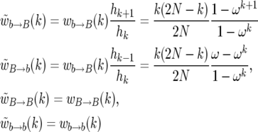
In this article, we consider only sweeps that succeed. It is thus necessary to consider the Markov chain conditioned on the success of the sweep. The conditioning does not change the rate of events replacing an individual for one of the same kind, since they do not affect the success of the sweep. The new rates become

(6)

(Durrett and Schweinsberg 2004), where ω = 1 − s. Thus, we can simulate the embedded Markov chain of the changes in k, conditioned on the success of the sweep if we take the probability p₊(k) of going from k to k + 1 copies of the B allele as

(7)

The probability that the number of alleles decreases from k to k − 1 is p₋(k) = 1 − p₊(k).

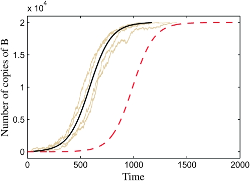
Figure 2 shows four realizations of the favored-allele frequency x(t) generated with the algorithm described above. Also shown is the logistic model for x(t) (dashed line), which is not a good approximation, as well as our new model described in averaging over realizations of the sweep (solid line).

Figure 2.—

Growth of the favored-allele frequency in the population (time is measured in generations). The population size is N = 10⁴, and the selection parameter is s = 0.01. Shown are four samples of the Moran process (gray lines), the logistic model (dashed red line), and our new deterministic model described in A deterministic model for x(t) (solid black line). The new deterministic approximation (Equation 26) is much closer to the Moran curves than the logistic approximation.

Gene genealogies of the neutral loci during the sweep:

Here we describe our implementation of the Moran model for simulating the gene genealogies of neutral loci in the neighborhood of a selected locus. The algorithm is divided into a forward and a backward phase.

In the forward phase, we generate the sequence of the number k of B alleles, forward in time, according to the conditioned Markov process described in the previous section: starting from k = 1, k is incremented with probability p₊(k) or decremented with probability 1 − p₊(k), until k = 2N. Because we either increase or decrease k, each value in the sequence is different from the previous one.

In the backward phase, the population is divided into two subpopulations with B or b alleles at the selected locus. At the end of the sweep, all ancestral lines are in the B population; this is the starting point for the backward phase. We trace the genealogies of the neutral loci backward in time by traversing the sequence of k values (obtained in the forward pass) in reverse; this guarantees that the time reversal of the Moran process is correct. Each time k changes, we generate a event if the new value of k is smaller than the old one. Correspondingly, we generate a event if k increases. Between each change in k, we generate the and events of the Moran chain (these events do not change k). The number m of such events has a geometric distribution, , where

(8)

The probability that the event is a replacement is

(9)

and, correspondingly, the replacements occur with probability . Finally, the time between each event is exponentially distributed with expected value (2N)⁻¹ in units of generations.

We now describe the effect of the events generated during the sweep on the gene genealogies of the neutral loci. In each event, we choose the line to die and the line to replace it randomly from the appropriate subpopulations. As we proceed backward in time, the dying line coalesces with its parent line (e.g., in a event, we pick the line to coalesce from the b subpopulation). With probability r, recombination occurs between the selected locus and the rightmost locus during the coalescent. In this case, the region between the selected locus and the recombination point coalesces with the chosen parent, and the second part of the neutral region, between the recombination point and the rightmost locus, coalesces with a parent chosen with uniform probability from the whole population. We assume that the neutral locus of interest is sufficiently small so that there is at most one crossover event in the region in each meiosis (the deterministic coalescent models, however, are not subject to this limitation since in these models the recombination rate can be arbitrarily high). For the values of r considered in this article this approximation is good. If necessary, it is straightforward to improve it, for instance, by simulating an explicit recombination process instead of simply assuming that no or one crossover occurs in the interval in each meiosis. One may also implement more realistic models of recombination, e.g., models that capture crossover interference (see, e.g., McPeek and Speed 1995, for a review); for the purpose of this article, however, the simplest model is sufficient.

When the simulation has reached the beginning of the sweep, there is exactly one line carrying the B allele, and the genetic material of this individual is ancestral to all genetic material trapped in the sweep. In addition, there may be a set of lines that have escaped the sweep because of recombination as explained in positive selection and genetic hitchhiking. We then follow the lines carrying genetic material from the sample back in time until the most recent common ancestor of each locus has been found for the sample. Since there is no selection in this part of the history, the Moran process is a coalescent where the rate (in units of events per generation) of two lines coalescing is n(n − 1)/2N, where n is the number of lines in the population, and the rate of recombination is r.

AVERAGING OVER REALIZATIONS OF THE SWEEP

Durrett and Schweinsberg (2004) have convincingly shown that it is necessary to consider the fluctuations of the favored-allele frequency (displayed in Figure 2) to accurately represent effects of the sweep on nearby loci.

We now explain how to efficiently and accurately average over such fluctuations. We motivate our method by an example: how to compute the probability that the first recombination event, if it occurs during the sweep, occurs with an individual not carrying the favored allele at the selected locus. In the background coalescent for neutral loci in the vicinity of a selected one we describe a coalescent process that makes use of the ideas described in this section.

An example:

We illustrate our approach by considering the conditional probability Q(r) that the first recombination event, if it occurs during the sweep, occurs with an individual not carrying the favored allele at the selected locus:

(10)

Q(r) depends on the realization of x(t) of the sweep of duration τ. For small values of r, it is unlikely that a given line experiences more than one recombination event during the sweep, and in this case Q(r) is approximately the probability that the line escapes the sweep.

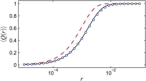
Figure 3 shows the average over realizations of x(t) as a function of r, obtained from Moran-model simulations (circles). Also shown are the results from the logistic model (dashed line), derived as follows. Inserting the solution of (1),

(11)

(where τ = 2 ln(2N − 1)/s is the duration of the sweep in the logistic model), into (10) and expanding the integrand in (10), we obtain

(12)

Figure 3.—

Comparison of as a function of r for the different models: Moran simulations (circles), the deterministic logistic model (dashed red line), and the new deterministic model (solid blue line). The population size is N = 10⁴ and the selection parameter is s = 0.01.

As can be seen in Figure 3, the result (12) deviates significantly from the Moran-model results.

We now show how to obtain a much more accurate approximation (solid line in Figure 3).

The problem in averaging (10) over different realizations of the stochastic Moran sweep lies in that both the upper bound τ of the integral and the integrand fluctuate. In the following we describe an approximate method of averaging (10) that gives accurate results and motivates a new deterministic model for selective sweeps. To begin with, note that x(t) is a piecewise constant function of time in the Moran model. A realization of the growth of the B allele is determined by a sequence of M pairs (k_i, τ_i), where k_i is the number of copies of B in time interval i, and τ_i is the duration of this interval (the latter begins at ). The sweep begins with k₁ = 1 at time t₁ = 0 and ends with k_M = 2N at time t_M. Thus, we have

(13)

The number M of steps in the growth process fluctuates and is usually ≫2N − 1 since k_i is usually not an increasing function of i.

We construct an increasing growth curve from the sequence (k_i, τ_i) as follows. First, consider the sequence obtained by sorting the intervals such that k_i ≤ k_i+1. Second, merging all intervals with the same value of k_i into one contiguous segment, we obtain a sequence of 2N − 1 segments, , with so that is the duration of the sweep. Note that may also be written as , which implies . 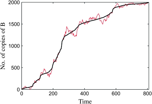This “sorted” sweep is monotonous: there are i copies of allele B in the population during the time interval , and at time the number of copies of B increases by one. Figure 4 shows that this results in a surprisingly accurate representation of the original trajectory x(t). This is so because of the conditioning on the success of the sweep: large downward fluctuations of k_i are rare.

Figure 4.—

Comparison between the actual growth curve k_i vs. t_i (red line) and the corresponding sorted curve vs. (black line). The parameters are N = 10³ and s = 0.01.

In terms of the sorted sweep, Equation 13 can be written as

(14)

Averaging (14) over the realizations of the sweep is straightforward. Assuming that can be approximated by , we find

(15)

The expectation values can be calculated analytically as shown in The expected value of below. In Figure 3, according to (15) is shown as a blue line, in very good agreement with the numerical data (circles).

A deterministic model for x(t):

Our result (15) can be written in the form (10) by introducing a deterministic model for the sweep. Let be the solution of for k. In Figure 2, is shown as a solid black line. Let . Then

(16)

where is the expected duration of the sweep.

In practice, is obtained as follows: we pick 10³ linearly spaced values for t in the interval [0,〈. For each value of t, we find the k such that 〈, using Equation 26 to calculate the values of . To find the value of corresponding to t, we use linear interpolation between the endpoints of this interval.

Results of coalescent processes based on the model for the selective sweep are summarized in the Conclusions. As expected the results obtained exhibit equally good agreement with our Moran-model simulation as does Figure 3.

The expected value of :

In this section, we derive an analytical expression for , the total time during the whole sweep when there are k copies of B or less, starting from a single copy. More generally, let T_i^(k) be the corresponding time, measured during the remaining parts of the sweep starting from i copies of B. Thus, we have 〈.

The value of equals the expected time until the next event, plus the expected time spent in states with k copies of B or less from the next state. Thus, we have the recursion

(17)

where θ_i is one if i ≥ 0 and is zero otherwise, and p_±(i) is the probability of going from i to i ± 1 copies of B; cf. Equation 7. To find a unique solution to (17), we need to provide boundary conditions. First, we note that the transition from i = 1 to i = 0 is forbidden (this is known as a “natural boundary condition”). Second, if the sweep is started at i = 2N it stops immediately; thus, we must take

(18)

for all k. In the following it turns out to be convenient to introduce

(19)

Writing (17) in terms of leads to a recursion with constant coefficients:

(20)

We solve (20) as follows. First, from (20) we obtain a recursion for the difference :

(21)

By telescoping from zero to i, we find the solution

(22)

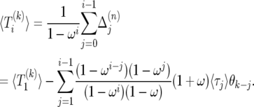
At i = 0, (19) implies , which leads to Δ₀ = . With this, summing (22) from 0 to i − 1 leads to

(23)

Setting i = 2N in (23), and using , we can solve for

(24)

Between each change in k, there is a geometrically distributed number of events. It follows from (8) that the expected time between two changes in k is

(25)

generations. Inserting the value of and writing the solution in terms of 〈, we obtain

(26)

Finally, we note that higher moments of , especially the variance, can be obtained in a similar manner.

THE BACKGROUND COALESCENT FOR NEUTRAL LOCI IN THE VICINITY OF A SELECTED ONE

As explained in positive selection and genetic hitchhiking, selection influences, via the hitchhiking effect, the evolution of neutral loci on the same chromosome as the selected locus. Given a particular growth of the favorable allele frequency x(t) as a function of time, what is the evolution of the linked neutral loci? The standard approach is to follow Kaplan et al. (1989) (see also Kaplan et al. 1988) in modeling the effect of selection on the neutral loci as a form of population structure: the selective sweep is viewed as a two-island population with migration, where one island, with population size 2Nx, contains the individuals with the B allele; the other island has population size 2N(1 − x) and contains the individuals with the b allele. Coalescent events can occur only between individuals on the same island. Recombination, however, may move a line from one island to the other, since the parent of the part of the neutral locus to the right of the recombination point is chosen uniformly from the whole population.

It is useful to write the total rate of coalescent and recombination events in the sample genealogy in the subdivided population in the form

(27)

where λ_B and λ_b are the total numbers of birth–death events per generation in the B and b subpopulations, respectively, given by

(28)

and where p_B and p_b are the probabilities that a single birth–death event leads to a coalescent or a recombination event (or both) involving an individual in the corresponding subpopulation.

Consider the probability p_B. First, a birth–death event has no effect on the gene genealogies unless the individual born is an ancestor to a locus of an individual in the sample. The probability that this is the case is simply n_B/(2Nx), where n_B is the number of ancestral lines currently in the B subpopulation. Second, for the gene genealogies to change either recombination must happen during the birth—this happens with probability r—or the parent must belong to a different ancestral line of the sample; the probability that this happens is (n_B − 1)/(2Nx). Since one of the subpopulations can be quite small, especially close to the ends of the sweep, we cannot make the usual assumption (Hudson 1990) that recombination and coalescence cannot occur in the same event. Putting it all together, we find

(29)

The first term corresponds to two lines coalescing in the B population with no recombination, and the second term corresponds to all events involving recombination.

We derive the probability p_b of an event in the b subpopulation in the same way as for p_B. The result is

(30)

where, correspondingly, n_b is the number of ancestral lines currently in the b subpopulation.

When x and the other parameters are constant, the coalescent is a Poisson process, and the time to the next event is exponentially distributed with expected value 1/λ_tot; see Equation 27. In a selective sweep, however, x changes with time; hence, the coalescent is an inhomogeneous Poisson process. The coalescent starts at the end of the sweep and creates a sequence of events for the sample genealogy at decreasing times, toward the beginning of the sweep. Given the state of the population at time t₁, the distribution f(t₂|t₁) of the time t₂ of the next event (t₂ < t₁) is

(31)

Hence, given that we have simulated the sweep from the end of the sweep to time t₁, the time t₂ of the next event is determined by solving the equation

(32)

numerically for t₂, where η is an exponentially distributed variable with expected value unity. For some simple growth models it is possible to find explicit analytical expressions for t₂ as a function of t₁ and η; mostly, however, one must use numerical approximations of the integral. In this article, we consider x(t) in (32) to be a given, piecewise constant function. Also when we have explicit expressions for x(t) it is convenient, and efficient, to take a number of samples at equally spaced points in time. We are then able to quickly find the interval containing the value of t₂ that solves (32) [if x(t) is piecewise constant, the left-hand side of (32) is piecewise linear and continuous].

This concludes our review of the standard background coalescent. There is only one problem with this picture: the rates λ_B and λ_b do not accurately describe the rate of birth–death events in the two subpopulations when we compare them to simulations using the Moran-model algorithm described in the moran model of positive selection: we observe slight but statistically significant deviations for large values of s (we find that the effect is negligible for s < 0.03 and is most significant when both s and r are relatively large).

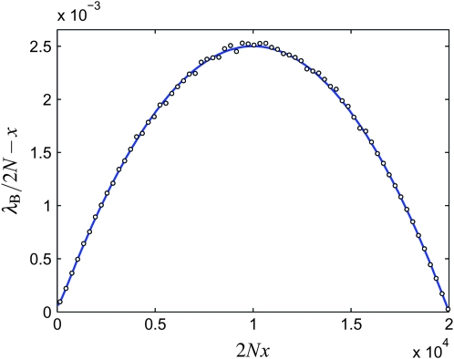
As is shown in Figure 5, the true birth rate of B alleles as a function of x in the Moran model is given by the total rate of all events leading to the birth of a B allele: combining Equations 2 and 6, we have

(33)

Figure 5.—

The birth rate of B alleles, λ_B, as a function of x for N = 10⁴, s = 0.01, and 10⁴ Moran simulations (white circles). Also shown is the theory (Equation 33, solid blue line). Note that the standard rates (Equation 28) correspond to λ_B = 2Nx.

Hence, the birth rate of B alleles is larger than expected from the standard model. Since the total number of events is fixed at 2N per generation, the birth rate of the b alleles is correspondingly smaller:

(34)

In general, we see that deviations from the standard rates are due to the difference in the birth rates of the two alleles. It is the selection process that causes extra births to happen in the B subpopulation and fewer births in the b subpopulation.

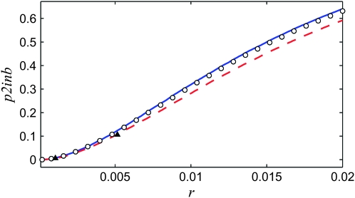
In Figure 6 we illustrate the difference between choosing the birth rates according to the standard method (28) and according to (33), by measuring the probability p2inb that two ancestral lines of a neutral locus escape the sweep separately. The parameters are N = 10⁴ and s = 0.1, corresponding to moderately strong selection. The background coalescent using λ_B from (33) is in good agreement with the Moran simulations, while the results using the rates (28) exhibit a small but significant difference. Other quantities exhibit similar differences (not shown).

Figure 6.—

Probability p2inb that two ancestral lines of a neutral locus escape the sweep separately, as a function of the amount of recombination r between the neutral and the selected locus. Shown are results of Moran-model simulations (circles) and results of the background coalescent with the growth x(t) given by sampling the Moran process for the selected locus, using either the standard rates in the literature (Equation 28) (red dashed line) or the new rates (Equations 33 and 34) (blue solid line). The coalescent simulations of Durrett and Schweinsberg (2004) (triangles) are consistent with the former, while our Moran model is much closer to the latter. The parameters are N = 10⁴ and s = 0.1.

RESULTS AND DISCUSSION

We have implemented the background coalescent for a contiguous segment of neutral loci close to a selected site (see the background coalescent for neutral loci in the vicinity of a selected one), using the deterministic model described in averaging over realizations of the sweep: is obtained by solving for k, as described in A deterministic model for x(t).

To establish the accuracy of our algorithm, we compare its results to those of Moran-model simulations. In particular, we compute the distribution over partitions at a neutral locus in the sample (Durrett and Schweinsberg 2004) (explained below in Partitions).

Duration of the sweep:

According to the results in The expected value of , we can use (26) to obtain a closed expression for , the expected duration of the sweep. Because of symmetry, we can write in the form

(35)

In the limit , we obtain the familiar result (see, e.g., Ewens 1979, for a review)

(36)

When 2Ns is large, we approximate ω^2N ≈ 0 and obtain to leading order

(37)

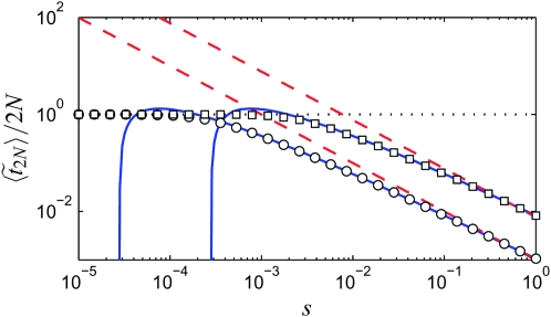
Here γ is Euler's constant, γ ≈ 0.577216. This approximation is excellent: as is shown in Figure 7, the approximation breaks down only when . Except for the γ-term, (37) is also the expected duration of the sweep one obtains in the diffusion approximation for the sweep conditioned on success (Etheridge et al. 2006, Lemma 3.1) and in the models by Barton (1998) and Kim and Nielsen (2004).

Figure 7.—

Comparison of the exact expression (Equation 35) (symbols), for the expected duration of the sweep (in units of 2N generations) as a function of s, to the approximation (cf. Equation 37) (solid blue lines) and the logistic model (solid red lines), for N = 10³ (squares) and N = 10⁴ (circles). As a reference, the result (Equation 36) is also shown (dotted line).

This result should be contrasted with the deterministic logistic sweep, where the duration of the sweep is 2 log(2N − 1)/s. For large values of s, the duration is close to that of the Moran model and to the approximation Equation 37. Thus, quantities depending primarily on the duration of the sweep, such as the amount of recombination taking place during the sweep, will be accurately described in the logistic model when the selection is strong. From (37), and in Figure 7, we see that this happens when is small compared to log(2N). When s is small, however, the duration of the sweep in the logistic model is very different from that of the Moran model, and consequently we expect a clear difference in the effect of the sweep on the neutral loci nearby.

Partitions:

Here we consider the distribution of partitions at a neutral locus at genetic distance r from the selected locus in a sample of two individuals in the population. The partitions are defined as follows (Donnelly 1986; Durrett and Schweinsberg 2004). Suppose we follow the ancestral lines of the neutral locus in the two individuals back in time through the sweep. Because of recombination, the lines may move from the B population to the b population and (with a rather small probability) back again. They may coalesce in one of the populations or stay separate during the whole sweep. For two lines, we have four distinct cases: both lines coalesce during the sweep and the resulting line is trapped by the sweep (the probability for this to happen is denoted by p2cinB); one line escapes the sweep and the other is trapped (p1B1b); both lines escape the sweep but do not coalesce (p2inb); the lines coalesce and then escape or escape separately and then coalesce (much less likely), denoted by p2cinb.

When the genetic distance to the selected locus is large, one expects all lines to escape independently. For large population sizes it is unlikely that lines coalesce during the sweep, but it becomes more common when the population size is relatively low (e.g., for N ∼ 10³). Close to the selected locus, nearly all lines are trapped in the sweep. The frequency of the case where one line is trapped and the other line escapes has a maximum for intermediate genetic distances r.

In Figure 8 we compare the four models: the Moran model, the logistic-sweep model, the DS algorithm, and our own algorithm, when N = 10⁴ and s = 0.1, corresponding to strong selection. Also shown are the coalescent simulations of Durrett and Schweinsberg (2004). The curves in Figures 8–10 were obtained by averaging over 10,000 samples. The plot covers the approximate range of validity quoted by Durrett and Schweinsberg (2004) for their algorithm, , which evaluates to ≈0.01. Over this range, all curves except the logistic model agree. In particular, the logistic model gives a higher value for p2cinb than expected; the most likely reason for this deviation is that the duration of the sweep is slightly too long in the logistic model (cf. Figure 7).

Figures 9 and 10 show the same quantities as Figure 8 but for s = 0.03 and s = 0.001, respectively. The range of validity of the DS algorithm is r < s/ln 2N, which is 0.003 in Figure 9 and 10⁻⁴ in Figure 10. Within this range, all curves except the logistic model agree approximately.

For larger values of r, the most important contribution to the difference between the Moran model and the DS algorithm is that the latter ignores recombination events and coalescent events during the middle and late stages of the sweep. As can be seen in the figures, this is a very good approximation provided r is sufficiently small or provided the sweep is sufficiently short. The accuracy of the logistic model quickly deteriorates as s decreases. Again, the most important reason is that the sweep is too long compared to the Moran model.

Our algorithm, by contrast works well also for large values of r and small values of s, although it is clear that the deviations from the Moran model become larger for smaller values of s. This is to be expected since the fluctuations of the sweep increase with decreasing s. In addition, we emphasize that each run of our program gives a realization for the joint gene histories of a contiguous stretch of DNA, while the DS algorithm requires a separate simulation for each value of r.

We conclude this section by comparing our model to the diffusion approximation of our Moran model. The SDE corresponding to the Moran model of the growth and fixation of the fraction x of the population with the favorable allele, with the rates given by Equation 6, is given by

(38)

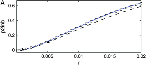
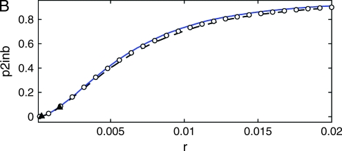
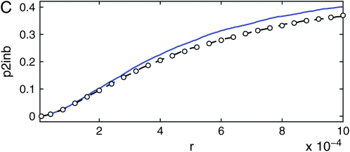
where dW is the differential of a Wiener process W (characterized by and dW² = dt) (see, e.g., Gardiner 2004 for more information). We simulate Equation 38 forward in time to obtain a trajectory x(t) starting at x(0) = 1/2N until fixation, i.e., until the first time x(t) > 1 − 1/2N. Given a realization of the curve x(t) we generate a sample gene genealogy using the standard structured coalescent. Although it is possible to time reverse the Moran process to avoid storing the path (Coop and Griffiths 2004), we perform the simulation forward in time. This allows us to use the same coalescent code as for the other models. Figure 11 shows the probability p2inb that both lines escape the selective sweep separately as a function of the genetic distance r between the neutral and the selected locus, from 10,000 samples, for three values of the selection parameter s (the other partitions, p2cinB, p2cinb, and p1B1b, exhibit similar differences between the models). The population size is N = 10⁴, and the selection parameters s = 0.1 (Figure 11A), s = 0.03 (Figure 11B), and s = 0.001 (Figure 11C). When selection is weak (Figure 11B), the diffusion approximation and our model are in close agreement with each other and with the Moran simulations. For very weak selection (Figure 11C), the diffusion approximation is more accurate. This is not surprising considering that the fluctuations of the duration of the sweep becomes increasingly important as the selection becomes weaker (but we still condition on the fixation of the advantageous allele). For stronger selection, however, our method is more accurate than the diffusion approximation that starts to show significant differences from the Moran model (Figure 11A).

Figure 11.—

The probability p2inb that both lines escape the selective sweep separately, as a function of the genetic distance r between the neutral and the selected locus, from 10,000 samples. The population size is N = 10⁴, and the selection parameters are s = 0.1 (A), s = 0.03 (B), and s = 0.001 (C). The data shown are Moran simulations (circles), integration of the SDE with the standard rates (dashed black line), our model (solid blue line), and coalescent simulations of Durrett and Schweinsberg (2004) (triangles).

Conclusions:

We have implemented a new model for genetic hitchhiking on the basis of a deterministic approximation for the growth of the favored-allele frequency during the selective sweep, in combination with a coalescent process for a locus (or set of loci) close to the selected locus. By comparison with direct Moran-model simulations we could show that our new model is very accurate. Two reasons for this success are that our model faithfully approximates the expected duration of the selective sweep and it is conditioned on the success of the sweep.

Our algorithm is as easily implemented as the standard logistic model, but is far more accurate, even applicable beyond the range of parameters given by Durrett and Schweinsberg (2004) for their algorithm. We have also shown that it compares favorably to the diffusion approximation of the Moran process, especially when selection is strong. For practical purposes it is important that the sweep is not assumed to happen instantaneously, so mutations occurring during the sweep are not neglected. Furthermore, the algorithm determines the fate of a contiguous segment of neutral loci in the vicinity of the selected locus, so that the method lends itself to the study of multilocus associations.

Our results have implications beyond the immediate context of this article. First, we introduced a new approximate representation of selective sweeps (the sorted sweep) that locally averages over fluctuations in the favored-allele frequency. We suspect that this approximation retains the fluctuations relevant for an accurate description of the genealogies of neutral loci close to the selected site. In which range of parameters this is true will be the subject of a subsequent study. Second, in the coalescent for the neutral loci, we have shown that the standard expression for the rates (Equation 28) must be modified. We expect that similar modifications are necessary in other cases, e.g., Moran models with changing population sizes, as, for instance, in population expansions and bottlenecks.

References

- Barton, N. H., 1998. The effect of hitch-hiking on neutral genealogies. Genet. Res. 72: 123–133. [Google Scholar]
- Braverman, J. M., R. R. Hudson, N. L. Kaplan, C. H. Langley and W. Stephan, 1995. The hitchhiking effect on the site frequency spectrum of DNA polymorphism. Genetics 140: 783–796. [DOI] [PMC free article] [PubMed] [Google Scholar]
- Coop, G., and R. C. Griffiths, 2004. Ancestral inference on gene trees under selection. Theor. Popul. Biol. 66: 219–232. [DOI] [PubMed] [Google Scholar]
- Donnelly, P., 1986. Partition structures, Polya urns, the Ewens sampling formula and the ages of alleles. Theor. Popul. Biol. 30: 271–288. [DOI] [PubMed] [Google Scholar]
- Durrett, R., 2002. Probability Models for DNA Sequence Evolution. Springer-Verlag, New York.
- Durrett, R., and J. Schweinsberg, 2004. Approximating selective sweeps. Theor. Popul. Biol. 66: 129–138. [DOI] [PubMed] [Google Scholar]
- Etheridge, A., P. Pfaffelhuber and A. Wakolbinger, 2006. An approximate sampling formula under genetic hitchhiking. Ann. Appl. Probab. 16: 685–729. [Google Scholar]
- Ewens, W. J., 1979. Mathematical Population Genetics. Springer, Berlin.
- Fisher, R. A., 1930. The Genetical Theory of Natural Selection, Variorum Ed. Oxford University Press, London/New York/Oxford.
- Gardiner, C., 2004. Handbook of Stochastic Methods for Physics, Chemistry, and Natural Sciences (Springer Series in Synergetics, Vol. 13, Ed. 3). Springer-Verlag, Berlin/Heidelberg, Germany/New York.
- Hudson, R. R., 1983. Properties of a neutral allele model with intragenetic recombination. Theor. Popul. Biol. 23: 183–201. [DOI] [PubMed] [Google Scholar]
- Hudson, R. R., 1990. Gene genealogies and the coalescent process, pp. 1–43 in Oxford Surveys in Evolutionary Biology, edited by D. Futuyma and J. Antonovics. Oxford University Press, Oxford.
- Hudson, R. R., 2002. Generating samples under a Wright-Fisher neutral model of genetic variation. Bioinformatics 18: 337–338. [DOI] [PubMed] [Google Scholar]
- Innan, H., and Y. Kim, 2004. Pattern of polymorphism after strong artificial selection in a domestication event. Proc. Natl. Acad. Sci. USA 101: 10667–10672. [DOI] [PMC free article] [PubMed] [Google Scholar]
- Kaplan, N. L., T. Darden and R. R. Hudson, 1988. The coalescent process in models with selection. Genetics 120: 819–829. [DOI] [PMC free article] [PubMed] [Google Scholar]
- Kaplan, N. L., R. R. Hudson and C. H. Langley, 1989. The “hitchhiking effect” revisited. Genetics 123: 887–899. [DOI] [PMC free article] [PubMed] [Google Scholar]
- Kim, Y., and R. Nielsen, 2004. Linkage disequilibrium as a signature of selective sweeps. Genetics 167: 1513–1524. [DOI] [PMC free article] [PubMed] [Google Scholar]
- Kim, Y., and W. Stephan, 2002. Detecting a local signature of genetic hitchhiking along a recombining chromosome. Genetics 160: 765–777. [DOI] [PMC free article] [PubMed] [Google Scholar]
- Kingman, J. F. C., 1982. The coalescent. Stoch. Proc. Appl. 13: 235–248. [Google Scholar]
- Maynard Smith, J., and J. Haigh, 1974. The hitch-hiking effect of a favourable gene. Genet. Res. 23: 23–35. [PubMed] [Google Scholar]
- McPeek, M. S., and T. P. Speed, 1995. Modelling interference in genetic recombination. Genetics 139: 1031–1044. [DOI] [PMC free article] [PubMed] [Google Scholar]
- Moran, P. A. P., 1958. Random processes in genetics. Proc. Camb. Philos. Soc. 54: 60–71. [Google Scholar]
- Nordborg, M., 2001. Coalescent theory, Chap. 7, pp. 179–212 in Handbook of Statistical Genetics, edited by D. J. Balding, M. Bishop and C. Cannings. John Wiley & Sons, New York.
- Otto, S. P., and N. H. Barton, 1997. The evolution of recombination: removing the limits to natural selection. Genetics 147: 879–906. [DOI] [PMC free article] [PubMed] [Google Scholar]
- Przeworski, M., 2002. The signature of positive selection at randomly chosen loci. Genetics 160: 1179–1189. [DOI] [PMC free article] [PubMed] [Google Scholar]
- Schweinsberg, J., and R. Durrett, 2005. Random partitions approximating the coalescence of lineages during a selective sweep. Ann. Appl. Prob. 15: 1591–1651. [Google Scholar]
- Slatkin, M., 2001. Simulating genealogies of selected alleles in a population of variable size. Genet. Res. 78: 49–57. [DOI] [PubMed] [Google Scholar]
- Stephan, W., T. Wiehe and M. W. Lenz, 1992. The effect of strongly selected substitutions of neural polymorphisms: analytical results based on diffusion theory. Theor. Popul. Biol. 41: 237–254. [Google Scholar]
- Wright, S., 1931. Evolution in Mendelian populations. Genetics 16: 97–159. [DOI] [PMC free article] [PubMed] [Google Scholar]