

Abstract
In this paper, we report a knowledge-based potential function, named the OPUS-Ca potential, that requires only Cα positions as input. The contributions from other atomic positions were established from pseudo-positions artificially built from a Cα trace for auxiliary purposes. The potential function is formed based on seven major representative molecular interactions in proteins: distance-dependent pairwise energy with orientational preference, hydrogen bonding energy, short-range energy, packing energy, tri-peptide packing energy, three-body energy, and solvation energy. From the testing of decoy recognition on a number of commonly used decoy sets, it is shown that the new potential function outperforms all known Cα-based potentials and most other coarse-grained ones that require more information than Cα positions. We hope that this potential function adds a new tool for protein structural modeling.
Keywords: knowledge-based potential function, decoy recognition, structure prediction, protein folding
Protein folding is one of the most challenging problems in both computational and experimental biophysics (Dobson and Karplus 1999). The goal is to determine three-dimensional structures from one-dimensional amino acid sequences. In computational studies, a potential function plays a central role in accurately predicting the structures. There are two general types of potential functions: One is physics-based and another is knowledge-based. The physics-based potential functions are derived from quantum mechanical calculations, e.g., the CHARMM force field (MacKerell et al. 1998), the essence of which is molecular mechanics. The knowledge-based potential functions are derived from statistical analysis of known protein structures, the essence of which is the potential of mean force, or free energy. In many applications, it has been shown that the knowledge-based potential functions outperform the physics-based ones. There are many comprehensive reviews for various potential functions in the literature (Sippl 1995; Jernigan and Bahar 1996; Moult 1997; Lazaridis and Karplus 2000; Gohlke and Klebe 2001; Meller and Elber 2002; Russ and Ranganathan 2002; Buchete et al. 2004a; Poole and Ranganathan 2006; Skolnick 2006; Zhou et al. 2006).
The knowledge-based potential functions can usually be divided into two types: atomic level potentials (DeBolt and Skolnick 1996; Zhang et al. 1997; Melo and Feytmans 1998; Samudrala and Moult 1998; Gatchell et al. 2000; Lu and Skolnick 2001; Zhou and Zhou 2002; McConkey et al. 2003; Hubner et al. 2005; Qiu and Elber 2005; Shen and Sali 2006) and coarse-grained potentials (Tanaka and Scheraga 1976; Miyazawa and Jernigan 1985; Hendlich et al. 1990; Sippl 1990; Hinds and Levitt 1992; Jones et al. 1992; Godzik et al. 1995; Miyazawa and Jernigan 1996; Bahar and Jernigan 1997; Eisenberg et al. 1997; Betancourt and Thirumalai 1999; Liwo et al. 1999; Simons et al. 1999; Tobi and Elber 2000; Melo et al. 2002; Zhang et al. 2003, 2004, 2006; Buchete et al. 2004b; Loose et al. 2004; Colubri et al. 2006; Dehouck et al. 2006; Dong et al. 2006; Rajgaria et al. 2006). The latter have been demonstrated to be highly effective in reducing the computational cost in modeling native protein structures, although they are sometimes thought not to be physically rigorous enough to reflect the entire landscape of the potential surface (Thomas and Dill 1996; Skolnick 2006). The performance and applicability of coarse-grained potential functions are largely modulated by the choice of a coarse-graining scheme. In many applications, an ability to accurately calculate the potential energy solely based on Cα positions would certainly give one some advantages. Typical examples are recent studies on modeling protein chain topology based on low-resolution density maps (Wu et al. 2005a) and on a coarse-grained folding simulation based on a Cα model (Wu et al. 2005b).
In this study, we have developed a knowledge-based potential function, named the OPUS-Ca potential, that requires only the Cα positions as input. The potential function contains seven terms for representing typical molecular interactions in proteins. They are distance-dependent pairwise energy with orientational preference, hydrogen bonding energy, short-range energy, packing energy, tri-peptide packing energy, three-body energy, and solvation energy. It was tested against a number of commonly used decoy sets. The results show that the OPUS-Ca potential outperforms all known Cα-based potentials and most other coarse-grained ones that require more information than Cα positions. We hope that this potential function adds a new tool for protein structural modeling.
Results
Performance of individual terms
We first demonstrate the performance of five major individual energy terms in Equation 1 (see Materials and Methods) in terms of decoy recognition. They are distance-dependent pairwise energy with orientational preference Epairwise, hydrogen bonding energy EHbond, short-range energy Eshort_range, packing energy Epacking, and solvation energy Esolvation. There are two other terms: tri-peptide packing energy Etri–peptide and three-body energy E 3–body. Due to their relatively small contributions, their individual performance is not presented in detail here.
The decoy sets used in this study were from two collections. One was the so-called Decoys'R'Us collection, which included decoy sets 4state_reduced (seven proteins) (Park and Levitt 1996), fisa (four proteins) (Simons et al. 1997), fisa_casp3 (five proteins) (Simons et al. 1997), lattice_ssfit (eight proteins) (Samudrala et al. 1999; Xia et al. 2000), and lmds (eight proteins) (Keasar and Levitt 2003). In total, there are 32 proteins in the Decoys'R'Us collection. Another collection was the LKF decoy set (185 proteins) (Loose et al. 2004).
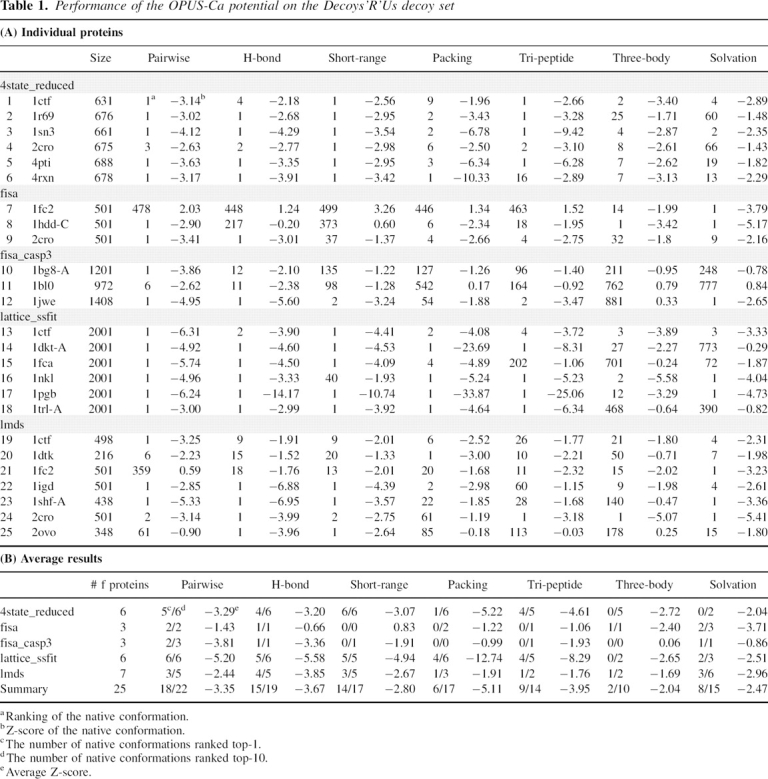
Table 1 gives the detailed ranking and Z-scores for individual proteins in the Decoys'R'Us collection. Note that only the results for 25 commonly used proteins in Decoys'R'Us (Tobi and Elber 2000; Dehouck et al. 2006) are listed.
Table 1.
Performance of the OPUS-Ca potential on the Decoys'R'Us decoy set
Distance-dependent pairwise energy with orientational preference
For the distance-dependent pairwise energy term Epairwise, the energy was calculated with respect to pseudo-Cβ atoms built from Cα atoms. In the literature (Zhang et al. 2004), it had been shown that pairwise energy based on Cβ atoms taken from X-ray structures was better than that based on Cα atoms because the distance between two Cβ atoms could better represent side chain packing than that between Cα atoms. This was confirmed in this study. Moreover, it has been shown that it is advantageous to include the orientational preference of residues (Buchete et al. 2004b; Miyazawa and Jernigan 2005). In this study, the pairwise energy in the OPUS-Ca potential took into account the relative orientation of two pairing residues. The comparison of decoy recognition for pairwise energy with and without orientation preference indicates that the energy with orientation preference could recognize the native conformation of more decoy sets than that without orientation preference. Also, the average Z-scores for the native structure in the two collections of decoy sets was observed to be 0.2–0.3 better in the case with the orientation preference than the case without. Figure 1 shows the performance on two decoy set collections, Decoys'R'Us (25 proteins) and LKF (185 proteins). The upper and middle panels give the percentage of proteins in the decoy sets whose native conformations were correctly ranked as the top 1 and within the top 10, respectively. It is clear that the trends in both decoy set collections are consistent; the performance of pairwise energy with pseudo-Cβ is better than the case without, and the performance of the energy with the orientational preference is better than the case without. Finally, the average Z-scores show exactly the same trend as well (Fig. 1, lower panels).
Figure 1.
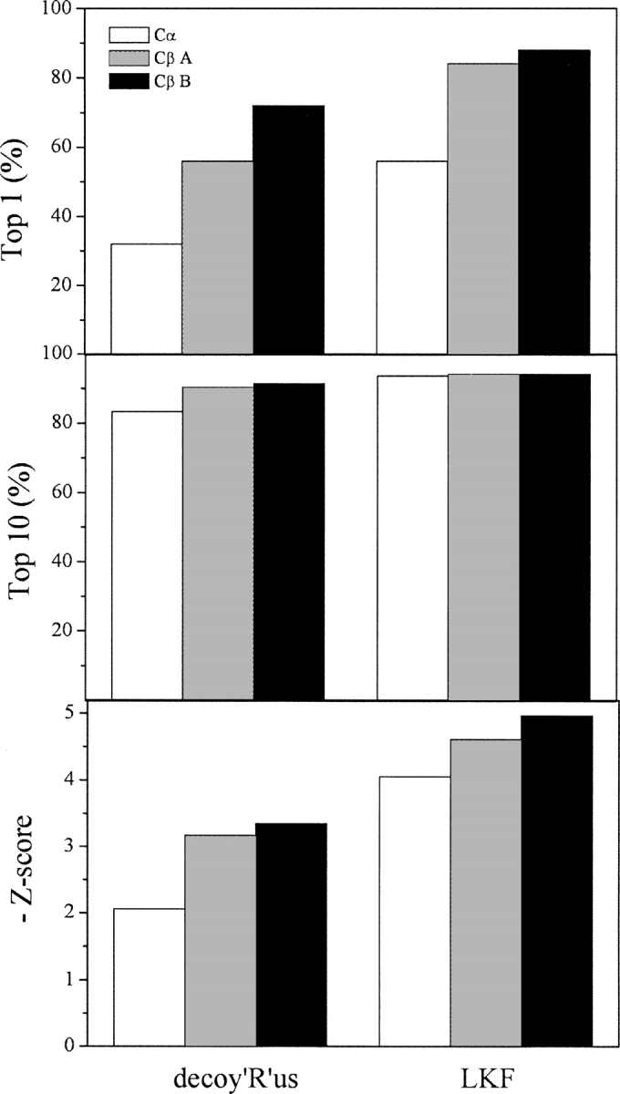
Performance of pairwise energy. (Top panel) Percentage of proteins in decoy sets whose native conformations were ranked top-1, (middle panel) percentage of proteins in decoy sets whose native conformations were ranked top-10, (bottom panel) the negative average Z-scores. (Cα) Pairwise energy based on Cα positions, (Cβ A) pairwise energy based on pseudo-Cβ positions built from Cα positions without orientation preference, (Cβ B) pairwise energy based on pseudo-Cβ positions built from Cα positions with orientation preference.
Hydrogen bonding energy
The hydrogen bonding energy term EHbond is required to build pseudo-backbone atoms from the original Cα atoms. They were the N and H atoms of amide groups and the C and O atoms of carbonyl groups. To compensate for error from building backbone atoms, the hydrogen bonding criteria were slightly modified. First, Cα-based hydrogen bonding energy was compared with all-atom-based hydrogen bonding energy, which directly used original backbone atoms and standard hydrogen bond criteria. By testing on 25 proteins in the Decoys'R'Us sets, it was found that Cα-based hydrogen bonding energy recognized more native conformations and had only a slightly lower Z-score than all-atom-based energy (Fig. 2). The Cα-based hydrogen bonding energy term also performed better than the all-atom-based calculation in the top-10 ranking.
Figure 2.
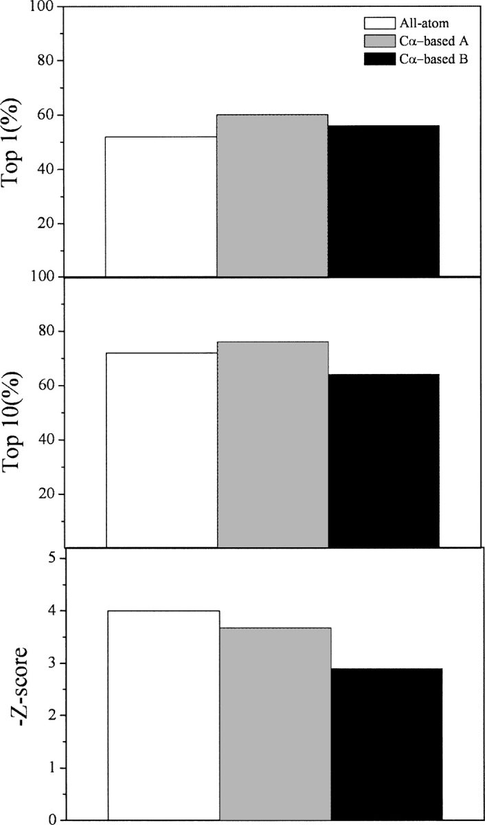
Performance of hydrogen bond energy. (Top panel) Percentage of proteins in decoy sets whose native conformations were ranked top-1, (middle panel) percentage of proteins in decoy sets whose native conformations were ranked top-10, (bottom panel) the negative average Z-scores. (All-atom) All-atom-based hydrogen bond energy, (Cα-based A) Cα-based hydrogen bond energy with an energy shift, (Cα-based B) Cα-based hydrogen bond energy without an energy shift. Results are shown for 25 proteins in the Decoys'R'Us collection.
Another feature of our hydrogen bonding energy was that an unfavorable energy barrier for hydrogen bond formation was eliminated by a constant energy shift. The occurrence of hydrogen bonds with a large CN distance and a large CON angle was rare. That caused hydrogen bonds to have higher energy at these regions than at the optimal hydrogen bonding region. The energy values sometimes could even be positive, so that hydrogen bond formation was not favorable. To better describe hydrogen bonding as an energetically favorable interaction, a constant energy shift was added to ensure that the energy was near zero when a hydrogen bond was about to form. Hence, hydrogen bonds could readily form without encountering an energy barrier when an amide group was close to a carbonyl group.
From Figure 2, one can see that, comparing with the case with a constant energy shift, the hydrogen bonding energy without a constant energy shift performed persistently worse in recognizing native conformation as top-1, top-10 ranking, and average Z-scores. It was also found that the ranking of the native conformations of three proteins (1nkl in lattice_ssfit, 1dtk in lmds, and 1fc2 in lmds) was dramatically worsened from within top-20 to below top-50. However, comparing with the case with an energy shift, it was found that our energy term performed worse in the lattice_ssfit and lmds decoy sets, while it performed better in the 4state_reduced and fisa decoy sets. So the effect of an energy shift was decoy-set-dependent, which was presumably related to how each decoy set was generated.
Short-range energy
For the short-range energy term Eshort_range, different types of secondary structures were considered separately. This was because residues in different secondary structure types had different preferences for local conformations. From Table 1A, one can see that the short-range energy could perform quite well in all decoy sets except for fisa and fisa_casp3 decoy sets, in which case it couldn't recognize any native conformation and only one in the top 10 (PDB code: 1jwe). This was probably because the decoys in fisa and fisa_casp3 were generated by Rosetta based on native small fragments (Simons et al. 1997); thus, the native-like nature of short-range conformations caused insensitivity in the energy term.
Packing energy
The packing energy term Epacking could be divided into seven smaller terms. They belong to three types: short-range packing that facilitated the formation of a single helix or single strand (EH_self, ES_self); long-range packing in paired strands that facilitated strand pairing (ES_pairing); and long-range packing between different helices or strands in stabilizing tertiary structure (EH–H_packing, EH–S_packing, ES–S_packing). Equal weight was used for all seven terms. At the i,i + 3 or i,i + 4 position in a single helix, Pro and Gly were less likely to be involved, as the EH_self was among the highest when packing pairs involved Pro and Gly. Ser, Thr, Asp, and Asn were the next four unfavorable residues. Also, Cys was less likely to pair with one of these four types of residues. In contrast, Ala was more likely to be involved in helices. It was also identified that Met–Met, Glu–Arg, and Glu–Lys pairs were favorable at both the i,i + 3 and i,i + 4 positions. A Met–Met pair had an EH_self of −1.086 and −1.149 at the i,i + 3 and i,i + 4 positions, respectively; a Glu–Arg pair had an EH_self of −1.333 and −1.275 at the i,i + 3 and i,i + 4 positions, respectively; and a Glu–Lys pair had an EH_self of −1.177 and −1.248 at the i,i + 3 and i,i + 4 positions, respectively. For the i,i + 2 position in a strand, Pro was identified to be unfavorable, while hydrophobic residues preferred these positions. For example, a Val–Val pair had an ES_self of −1.793, and a Val–Ile pair had an ES_self of −1.677. For two paired strands, packing residues tended to have hydrogen bond and electrostatic interactions. Preferred contacting residues contained Cys–Cys, Glu/Asp–Arg/Lys, His–His, Ser–Asn/Gln, Trp–Trp pairs, etc. For example, ES_pairing (averaged over seven cases) for Cys–Cys was −0.811; ES_pairing (averaged over seven cases) for Glu–Arg was −0.894; ES_pairing (averaged over seven cases) for His–His was −0.605. For long-range tertiary packing, it was found that hydrophobic and large aromatic residues were favorable. For example, Tyr–Trp had an ES–S_packing of −2.470, and Ile–Leu had an EH–H_packing of −1.687.
The overall performance of the packing energy term in Decoys'R'Us recognized six native conformations in the top-1 ranking and 17 in the top-10 ranking (Table 1).
Solvation energy
The solvation energy term Esolvation was based on side chain solvent-accessible surfaces (SAS). An all-atom-based energy function was first established based on the SAS calculated from an all-atom model. Then, the SAS for the Cα model was estimated based on a coarse-grained method in which all parameters involved were systemically optimized from a structure database (see Materials and Methods). Using this estimated SAS as an approximate value, the solvation energy for the Cα model can be estimated from the all-atom-based energy function.
As indicated in Figure 3, in the Decoys'R'Us test, solvation energy based on an all-atom SAS found native conformations of 11 decoy sets in the top-1 ranking, and 22 native conformations in the top-10 ranking. This implied reasonable accuracy of the solvation energy term when the SAS was obtained from the all-atom structure. For the Cα model, the energy function was not as good as its all-atom counterpart. However, it still recognized eight native conformations in the top-1 ranking and 15 in the top-10 ranking. The average Z-scores are also listed in Figure 3.
Figure 3.

Performance of solvation energy. (Top panel) The negative average Z-scores, (bottom panel) the number of proteins in decoy sets whose native conformations were ranked top-1 (left) and top-10 (right). (All-atom) Solvation energy based on the solvent-accessible surface calculated from all atom positions, (Cα-based) solvation energy based on the solvent-accessible surface calculated from Cα positions only. Results are shown for 25 proteins in the Decoys'R'Us collection.
Performance of the overall energy function
To examine the performance of the overall energy function, weights had to be assigned to seven energy terms, a procedure that could sometimes be subjective. Two different ways of weight assigning were tried.
In the first way, all energy terms were calculated for all proteins in a non-homology database that had no chain break (a total of 1673 proteins [Wang and Dunbrack Jr. 2003]). The average energy was calculated for each term. Weights were assigned in such a way that they were anti-proportional to the average energy so as to make the numerical contribution from each term roughly equal. As indicated in Table 2, this scheme of weight assignment resulted in 18 out of 25 decoy sets in Decoys'R'Us with their native conformations correctly recognized as the lowest in energy (Subset 1 in Table 2). In the LKF decoy collection (Subset 2 in Table 2), it recognized 148 out of 151 decoy sets. As the tri-peptide and three-body energy terms could be regarded as higher order corrections of other terms, we also empirically lowered the magnitudes of these two weights to 0.1. It was found that the energy function with the modified weights could slightly improve the performance (19 out of 25 Decoys'R'Us decoy sets), indicating the less important nature of these two terms.
Table 2.
Weights and performance in decoy set recognition

In the second way, all seven weights were optimized iteratively on three subsets of decoy sets (see Materials and Methods). Strikingly, it was found that the magnitudes of the optimized weights were very close to the modified weight mentioned above. With the optimized weights, the energy function could recognize 21 native conformations out of 25 decoy sets in Decoys'R'Us and 146 native conformations out of 151 LKF decoy sets. The performance in Subset-3 was also similar. Overall, the performance with the optimized weights was close to the case with the modified weight. This result indicates that the optimized weights are not very biased by the weight optimization procedure. We suggest using optimized weights in real applications as they have included the most diverse features of all decoy sets.
The correlation between the root mean square deviation (RMSD) of decoy conformations from the native conformation and the energy of decoy conformations was evaluated. As indicated in Figure 4, a most linear-like correlation between the RMSD and energy was observed for 4state_reduced. Decoy set LKF had reasonable correlations. However, in other decoy sets the correlations were not so good. This suggests that the correlation between RMSD and energy depended on how the decoy sets were generated.
Figure 4.

Scatter plots of total energy vs. RMSD of decoy from the native structure (based on Cα atoms). Results of eight proteins (1r69 and 4pti in the 4state_reduced decoy set, 1hdd-C in the fisa decoy set, 1jwe in the fisa_casp3 decoy set, 1fca in the lattice_ssfit decoy set, 2cro in the lmds decoy set, and 1bg8, 1bo0 in the LKF decoy set) are shown.
The performance of the OPUS-Ca potential was also compared with that of other potentials. In the literature, there are a few energy functions solely based on Cα atoms (Loose et al. 2004; Rajgaria et al. 2006; Zhang et al. 2006). The results are listed in Table 3. The performance of the OPUS-Ca potential seems to be better in terms of decoy set recognition and Z-scores. It also outperformed many other coarse-grained potential functions that require more information than Cα positions (Hinds and Levitt 1992; Godzik et al. 1995; Miyazawa and Jernigan 1996; Bahar and Jernigan 1997; Betancourt and Thirumalai 1999; Tobi and Elber 2000; Zhang et al. 2004; Dong et al. 2006). In two cases (Zhou and Zhou 2002; Dehouck et al. 2006), the performance was similar.
Table 3.
Comparison of performance between OPUS-Ca and other potential functions

Discussion
In this study, a knowledge-based potential function, named the OPUS-Ca potential, was developed. To evaluate the potential function, only Cα positions are needed as input. Since it is hard to establish a sensitive enough potential function based only on Cα positions, the contributions from other atomic positions were established from pseudo-positions artificially built from the Cα trace. The potential function was constructed based on seven major terms representing dominant molecular interactions in proteins. The seven terms are distance-dependent pairwise energy with orientational preference, hydrogen bonding energy, short-range energy, packing energy, tri-peptide packing energy, three-body energy, and solvation energy.
Decoy set recognition indicated that the overall potential function outperformed all known Cα-based potentials and most of the other coarse-grained ones that require more information than Cα positions. For the performance of individual terms, it was found that the distance-dependent pairwise energy with orientational preference performed the best, which could identify 18 native conformations alone (out of 25 proteins in the Decoys'R'Us collection). Hydrogen bonding and short-range energy could also identify 15 and 14 native conformations, respectively. If the top-10 was used for native conformation ranking, then five out of seven energy terms could identify >15 native conformations alone (especially, the distance-dependent pairwise energy with orientational preference could identify 22 native conformations). The performance of some individual terms could even perform better than some of the other potentials published in the literature. This highly optimized performance of individual terms is advantageous because, in certain situations, one may want to use the individual energy terms separately based on their physical nature.
An important and difficult issue in developing knowledge-based potential functions is the assignment of weight for each term (Feng et al. 2007). In general, each term represents one or more aspects of physical interactions, so the contribution of each term should be inherently determined by the physical features of protein structures. Ideally, the magnitudes of weights should be independent of their performance on decoy sets, and independent of the methods in generating decoy sets. However, there is no ab initio way to determine the contribution of each energy term. Besides, some energy terms, like pairwise, three-body, and tri-peptide terms, have a mixture of several basic physical interactions; i.e., they are not completely orthogonal to each other. That makes weight optimization even more subjective. This is why weight optimization by using a specific training set often introduces biases. In this study, several different ways of assigning weights were tried in order to minimize the bias.
Materials and Methods
The total energy function consists of seven terms,
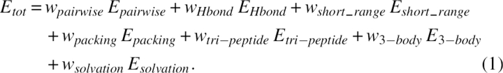 |
Here, w is the weight for that energy term. The statistical analysis of the knowledge-based potential function was performed over a nonhomologous structure database from the PISCES server by Dunbrack (Wang and Dunbrack Jr. 2003). Only X-ray structures were used. The percentage identity cutoff was 30%. The resolution cutoff was 1.8 Å. The R-factor cutoff was 0.25. The total number of chains was 2232.
Building pseudo-main chain atoms
Although the energy function only requires a Cα trace as input, to reliably build some of the terms in Equation (1), pseudo-main chain (including N, C, O, and H atoms) and Cβ conformations were established from a Cα trace. The procedure was based on the observation that main chain conformation can be mostly determined by local conformation of Cα atoms (Fidelis et al. 1994; Milik et al. 1997). In general, a main chain atom database was established, and it contained positional information of main chain atoms with respect to the local conformation of Cα atoms extracted from the nonhomologous structure database.
In detail, all main chain atoms of residue i were built from the position of four consecutive Cα atoms of residues i − 1, i, i + 1, and i + 2. The local Cα conformation was based on three parameters: Cα−Cα distance (di −1,i+1) between residues i − 1 and i + 1, Cα−Cα distance (d i,i+2) between residues i and i + 2, and the dihedral angle (φi) formed by all four Cα atoms. Figure 5 schematically illustrates these parameters. Here, the distance was divided into 10 bins with a bin width of 0.3 Å. The range of the distance in the analysis was 4.6–7.6 Å. The dihedral angle was divided into 36 bins with a bin width of 10°. This led to a total of 10 × 10 × 36 = 3,600 three-dimensional bins. To establish the main chain atom database, the positions of all main chain atoms (N, C, O, H) found in the structure database were averaged within each bin. To perform the averaging, a local reference frame was used. Its origin was set at the Cα atom of residue i, and Cartesian coordinate axes v x, v y, v z were defined as:
Figure 5.

Schematic illustration of parameters used to build pseudo-main chain atoms and Cβ atoms from Cα positions. The three parameters are the Cα−Cα distance (di −1,i+1) between residues i − 1 and i + 1, the Cα−Cα distance (d i,i+2) between residues i and i + 2, and the dihedral angle (φi) formed by all four Cα atoms. v x, v y, v z are local Cartesian coordinate axes to build atoms.
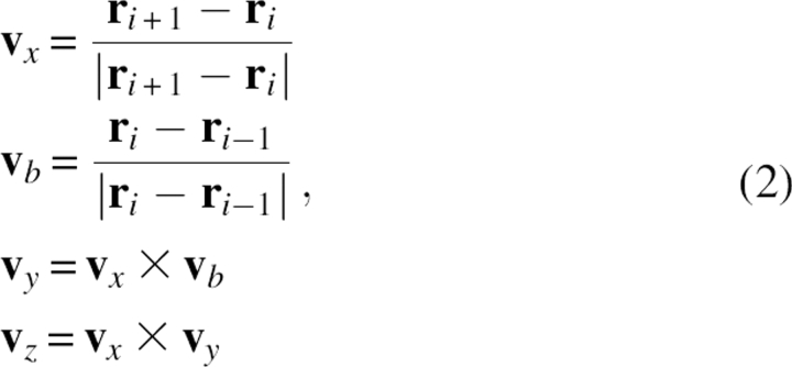 |
where r i was the Cα positional vector of residue i and v b was an auxiliary vector.
In addition, if the Cα distance between residues i and i + 1 was 2.7–3.3 Å, e.g., the cis-peptide bond in the case such as proline, statistical analysis of the histogram was performed separately. In the case where not enough statistical data were available for a particular bin, data from the most similar bins were assigned. For the first and last two residues, their local Cα conformations were assumed to be the same as those of the nearby residues so that their main chain atoms could be built as well (note, for most proteins, these residues were highly flexible). Also, to build the main chain atoms between the first Cα and second Cα atoms, local reference coordinate axes v′x, v′y, v′z on the first Cα atom were defined as
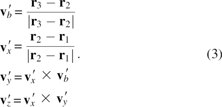 |
In a real application, given the conformation of four consecutive Cα atoms, one would look up the corresponding bin based on the distances and dihedral parameters, and assign the main chain atoms coordinates extracted from the database. After establishing the positions of the main chain atoms, Cβ atoms could be built from the N, Cα, and C atoms according to the standard parameters: The bond length of the Cα−Cβ bond was 1.53Å, the bond angle of the N-Cα−Cβ angle was 110°, and the dihedral angle between plane N-Cα-C and plane Cα-C-Cβ was 124°.
Distance-dependent pairwise energy with orientational preference
The term Epairwise was the distance-dependent pairwise energy term. It had an orientational preference in such a way that cases in which the side chain of one residue points away from the partner residue and points toward the partner residue were distinguished. Specifically, a Cα to Cβ vector was used to represent the rough direction of the side chain. The distance-scaled finite ideal-gas reference state was used to normalize the statistical data (Zhou and Zhou 2002). For a pair of residues whose Cβ atoms were within the cutoff distance (rcut = 15Å), the energy Epairwise for residues i with respect to residue j was given by
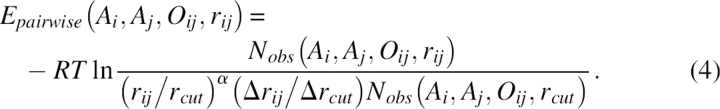 |
Here, Ai was the residue type, rij was the Cβ−Cβ distance between residues i and j, and Δrij and Δrcut were the bin width at distance rij and rcut. The constant R was the gas constant and T was temperature (both were set to 1 in practice). The total number of bins used in the study was 20. The bin width was 2 Å for rij < 2 Å, 0.5 Å for 2 Å < rij < 8 Å, and 1 Å for 8 Å < rij < 15 Å. The exponent α was 1.61. The term Nobs(Ai, Aj, Oij, rij) gave the observed number of pairs of Cβ atoms at the designated distance in their respective orientation in the structural database. The symbol Oij was expressed as
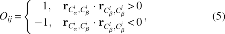 |
where r atom1,atom2 was the displacement vector from atom 1 to atom 2. The symbol Oij was used to distinguish the effect of the relative orientation of the two residues. If the value of Oij was 1, residue i pointed toward residue j; if the value of Oij was −1, residue i pointed away from residue j. Note this means that the case of i pointing toward j and the case of j pointing toward i can be different. Figure 6 schematically illustrates the two cases; in panel A, residue i points toward j, but residue j points away from i. In panel B, both residues point toward each other. Because of the normalization, the energy term Epairwise naturally decays to zero at cutoff distance rcut. In the case of glycine, Cα atoms were used instead, and the effect of orientation was omitted.
Figure 6.

Schematic illustration of the different orientations of interacting Cβ pairs. (A) Residue i points toward j, but residue j points away from i. (B) Both residues point toward each other.
Hydrogen bonding energy
The term EHbond was the main chain hydrogen bonding energy. It was developed first via statistical analysis of those residue pairs in the nonhomologous structure database based on an all-atom structure model. Then, for Cα models in real applications, the energy was computed based on the constructed pseudo-backbone atom positions.
The hydrogen bonding criterion based on the all-atom structure model was from Fabiola et al. (2002),
Figure 7 illustrates the parameters. For a particular pair distance rij = rC,N and interaction angle θij = ∠CON, the total number of main chain hydrogen bonds was counted as N(rij,θij) in a space region defined from (rij,θij) to (rij + Δrij, θij + Δθij) with volume V(rij,θij) (Δrij was 0.1 Å and Δθij was π/36). This region was cylindrically symmetric with respect to the main chain carbonyl bond (it was assumed that the nitrogen atoms in hydrogen bonding interactions in this region were uniformly distributed). Then, the hydrogen bonding energy EHbond as a function of (rij,θij) was given by
Figure 7.

Schematic illustration of the parameters used in H-bond energy. ∠CON, ∠NHO, rO,N, rO,H are used in hydrogen bonding criterion. ∠CON, rC,N are used as energy parameters.
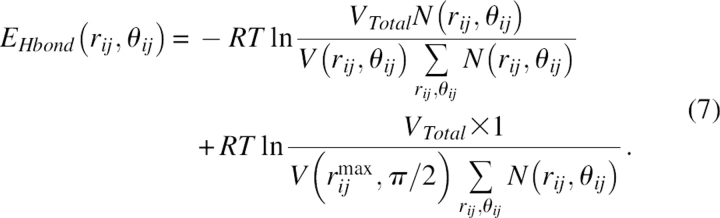 |
Here, VTotal was the volume of the entire search space defined as the spherical shell with rij in the range of 1.8–3.3 Å, rij max was 4.8 Å, and θij was in the range of [0,π]. The sum in the denominator gave the total number of hydrogen bonding pairs in the research region. The counting only applied to residues that were at least two residues apart in sequence. The second part of the energy term was a constant energy shift to eliminate the energy barrier during hydrogen bond formation. Note that in this study, proline was never considered a donor, and chain C termini were never considered as acceptors.
In real applications, main chain atoms (including hydrogen atoms) were built from Cα atoms first. It was found that the N and C atoms built from Cα atoms had ∼0.1 Å RMSD from native positions, while O atoms had ∼0.3–0.4 Å. In order to avoid the wrong assignment of hydrogen bonds owning to the error of the estimated main chain, a modified criterion was used:
It was found that by using this criterion, ∼91% of the hydrogen bonds identified by the old criterion in Equation 6 were found by the new criterion in Equation 8. Thus, the current only-Cα-based method could provide a reasonably close energy value to the all-atom main chain hydrogen bond energy.
Cα-based secondary structure assignment
Several terms in the energy function required the secondary structure assignment. The Cα trace alone does not allow one to accurately identify the secondary structure by methods such as the DSSP algorithm (Kabsch and Sander 1983), and the positions of main chain atoms built were pseudo-positions for auxiliary purposes; i.e., they were not accurate enough for regular secondary structure assignment. As indicated above, a modified definition of hydrogen bonds was used for DSSP analysis. Since, with the new definition, only 9% of hydrogen bonds were missed, it was expected that the accuracy of the secondary structure assignment on the sole Cα level would be reasonable. Only three types of secondary structure elements were used: α-helix, 10–3 helix, and π-helix were categorized as helix; extended sheet and β-bridge were categorized as sheet; others, such as loop and bend, were categorized as loop.
Short-range term
The term Eshort_range is a short-range energy term. The conformation of each pentapeptide fragment was divided into discrete bins, associated with the sequence information. The correlation between the sequence and local secondary structure for each pentapeptide fragment was constructed and transferred into energy functions based on the statistical distribution extracted from the nonhomologous structure database. This short-range energy term presents the structural preference of local fragments.
The conformation of the Cα trace for a protein of N residues was thus defined by 3N − 6 parameters: N − 1 pseudo-bonds connecting two neighboring Cα atoms, N − 2 pseudo-bond angles (θ) formed by three Cα atoms, and N − 3 pseudo-dihedral angles (φ) formed by four Cα atoms. All the degrees of freedom are illustrated in Figure 8. The energy function was expressed as:
Figure 8.

Schematic illustration of short-range parameters. θ is the pseudo-bond angle formed by three consecutive Cα atoms; φ is pseudo-dihedral angles formed by four consecutive Cα atoms.
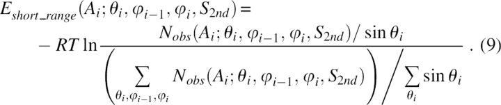 |
Here, Ai was the residue type of the central residue in the pentapeptide (20-letter code) and S 2nd was the secondary structure type. The bond angle, which was from 0°–180°, was divided into six bins. The dihedral angle, which was from −180° to 180°, was divided into 24 bins.
Packing term
The term Epacking was for pairwise packing energy related to the side chain orientation, residue type, and secondary structure. The packing energy can be expressed as a sum of six terms,
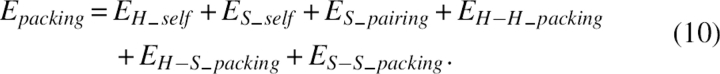 |
The first term, EH_self, was the helix self-packing energy. Side chain interactions within a helix have been analyzed previously (Stapley and Doig 1997; Adamian and Liang 2001; Andrew et al. 2001; Shi et al. 2002), and (i,i + 3), (i,i + 4) residue pairs play a significant role in stabilizing helix structure. Hence, the sequence propensity of such residue pairs in a helix was statistically analyzed in the structure database. The term EH_self can be expressed as:
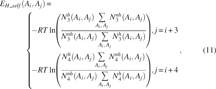 |
where N 3 h(Ai, Aj) was the number of cases in which residue i of type Ai was three residues ahead in sequence of residue j of type Aj on the helix, N 3 nh(Ai, Aj) was for the cases in which both residues were not in the helix, N 4 h(Ai, Aj) was the number of cases in which residue i of type Ai was four residues ahead in sequence of residue j of type Aj in the helix, and N 4 nh(Ai, Aj) was for the cases in which both residues were not on the helix.
The second term, ES_self, is sheet self-packing energy, very similar to the first term. The sequence propensity of (i,i + 2) residue pairs in a sheet was statistically analyzed in the structure database. So,
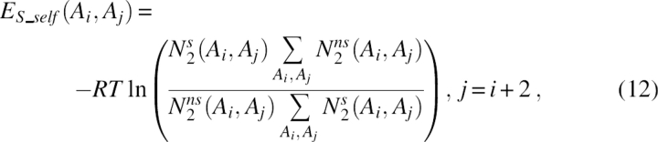 |
where N 2 s(Ai, Aj) was the number of cases in which residue i of type Ai was two residues ahead in sequence of residue j of type Aj on the strand, and N 2 ns(Ai, Aj) was for the cases in which both residues were not on the strand.
The third term, ES_pairing, was the intrasheet strand–strand pairing energy. In this term, the sequence propensity of any interacting residue pair in both antiparallel and parallel cases was analyzed. Comparing with what has been reported in the literature (Hutchinson et al. 1998; Steward and Thornton 2002), a more complete set of interacting types for residue pairs was included. This energy term is very useful in determining the sequence register of pairing β-strands. Let Tij denote the type of interacting residue pairs i, j. There were in total four types of interacting residue pairs for the antiparallel sheet (schematically shown in Fig. 9A): a hydrogen-bond-involving pair (type AA, Tij = (0, 0)), a non-hydrogen-bond-involving pair (type aa, Tij = (1, 1)), a hydrogen-bond-involving residue interacting with the next hydrogen-bond-involving residue on the opposite strand [type AB, Tij = (0,2)], and a non-hydrogen-bond-involving residue interacting with the next non-hydrogen-bond-involving residue on the opposite strand [type ab, Tij = (1,3)]. Similarly, there were three types of interacting residue pairs for the parallel sheet (schematically shown in Fig. 9B): a hydrogen-bond-involving residue interacting with a non-hydrogen-bond-involving residue [type Aa, Tij = (0,1)], a hydrogen-bond-involving residue interacting with the next non-hydrogen-bond-involving residue on the opposite strand toward the C terminus [type Ab, Tij = (0,3)], and a non-hydrogen-bond-involving residue interacting with a hydrogen-bond-involving residue on the opposite strand toward the C terminus [type aB, Tij = (3,0)]. Note that the four types in the antiparallel sheet were symmetric, while the three types in the parallel sheet were asymmetric with respect to the direction of the polypeptide chain. The term ES_pairing could be expressed as:
Figure 9.
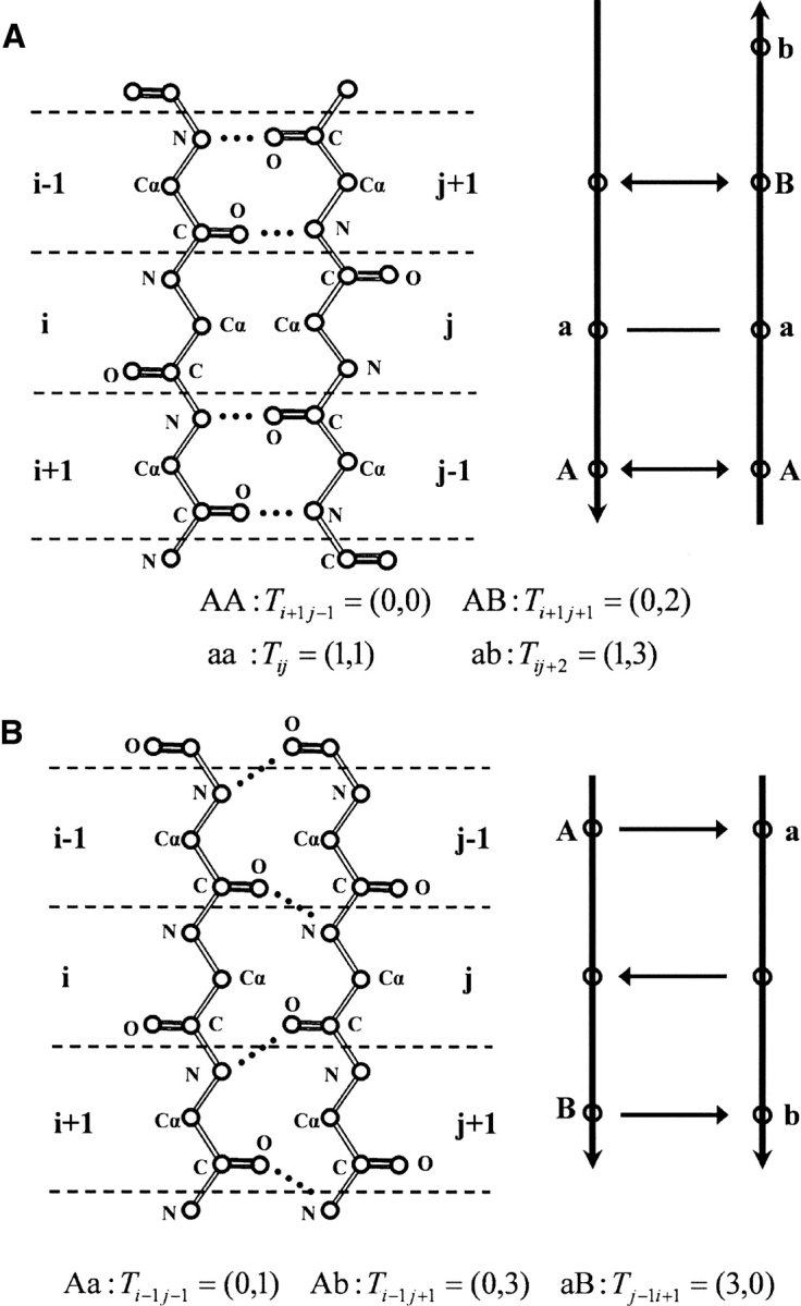
Seven types of interacting residue pairs in two pairing β-strands. (A) Four types of interacting residue pairs in antiparallel β-strands. (AA) A hydrogen-bond-involving pair [Ti +1j−1 = (0,0); note for illustration purposes that the subscripts of Tpq are based on the diagram in the figure]; (aa) a non-hydrogen-bond-involving pair [Tij = (1,1)]; (AB) a hydrogen-bond-involving residue interacting with the next hydrogen-bond-involving residue on the opposite strand [Ti +1j+1 = (0,2)]; (ab) a non-hydrogen-bond-involving residue interacting with the next non-hydrogen-bond-involving residue on the opposite strand [Tij +2 = (1,3)]. (B) Three types of interacting residue pairs in parallel β-strands. (Aa) A hydrogen-bond-involving residue interacting with a non-hydrogen-bond-involving residue [Ti −1j−1 = (0,1)]; (Ab) a hydrogen-bond-involving residue interacting with the next non-hydrogen-bond-involving residue on the opposite strand toward the C terminus [Ti −1j+1 = (0,3)]; (aB) a non-hydrogen-bond-involving residue interacting with the next hydrogen-bond-involving residue on the opposite strand toward the C terminus [Tj −1i+1 = (3,0)].
 |
where Nobs(Ai, Aj, Tij) was the observed number of one specific interacting residue pair of type Ai and Aj.
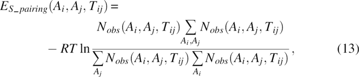
The fourth term, EH–H_packing, was the interhelix packing energy. The sequence propensity of the packing residue pairs in different helices was analyzed. The strategy was to define a Cα-based condition for interhelix packing, then to develop an energy term based on that. First, a residue-type-dependent cutoff distance, dcuthh(Ai,Aj), was defined as the distance between the Cβ (or Cα in the case of glycine) of two residues for an interhelix interaction. To determine dcuthh(Ai,Aj), the distances between the Cβ atoms (or Cα in the case of glycine) of two residues in different helices whose side chains had contacts was analyzed in the structure database. Two side chains were considered to have contacts if the distance between two atoms from each side chain was <5 Å. The cutoff distance dcuthh(Ai,Aj) was chosen to include most of the contacting residue pairs while having reasonably low false positives, and its value was kept in a lookup table. The interhelix packing criterion based on the pseudo-Cβ position was:
 |
The energy term can be expressed as:
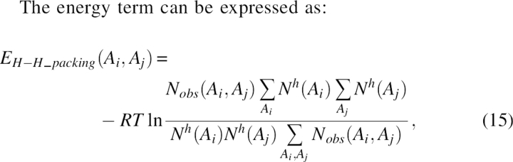 |
where Nobs(Ai, Aj) was the observed number of interacting packing pairs in a helix of residues of type Ai and Aj, and Nh(Ai) was the total number of residues of type Ai in the helix.
The fifth term, EH–S_packing, was the helix-strand packing energy. The helix-sheet packing criterion was almost the same as the interhelix packing criterion in Equation 14, except that the cutoff distance dcuths(Ai,Aj) for helix-strand packing was extracted from the structure database. The energy term can be expressed as:
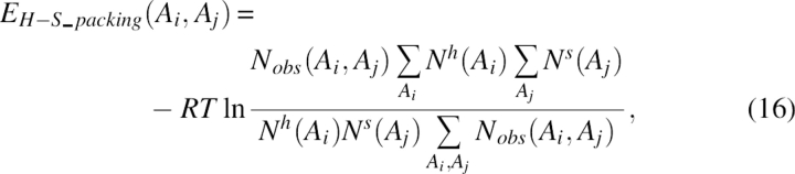 |
where Nobs(Ai, Aj) was the observed number of interacting packing pairs for two residues of type Ai in a helix and Aj in a sheet, Nh(Ai) was the total number of residue of type Ai in a helix, and Ns(Aj) was the total number of residues of type Aj in a sheet.
The sixth term, ES–S_packing, was the intersheet strand–strand packing energy. Differing from the third term, this term represented the sequence propensity of packing residue pairs in different β-sheets. The criterion of packing residue pairs in strand–strand packing was:
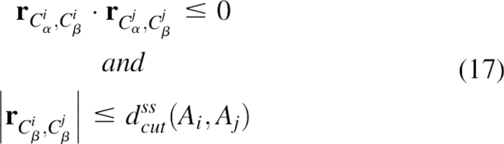 |
where dcutss(Ai,Aj) was the cutoff distance extracted from the structure database. Note that the residue pairs belonging to two contacting strands in the same sheet were excluded. The energy term can be expressed as:
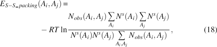 |
where Nobs(Ai, Aj) was the observed number of interacting packing pairs in a sheet for two residues of type Ai, Aj, and Ns(Ai) was the total number of residues of type Ai in a sheet.
Tri-peptide packing term
The term Etri–lpeptide was for the tri-peptide energy, defined as the contact energy of two specific tri-peptides with corresponding secondary structure types. The amino acids were grouped into four categories based on their physicochemical properties and sizes: (Asp, Glu, Lys, Arg, His), (Ser, Thr, Asn, Gln), (Gly, Ala, Val, Cys, Met), and (Ile, Leu, Pro, Phe, Tyr, Trp). Three types of secondary structure, α-helix, β-strand, and loop, were used. Therefore, there was a total of 64 × 3 = 192 different types of tri-peptides, in which 64 = 4 × 4 × 4 was for the coarse-grained residue types, and three was for the secondary structure types. The tertiary packing potential was given by
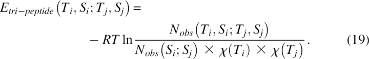 |
Here, Ti was for the ith tri-peptide, Si was for the secondary structure type of that tri-peptide, and χ(Ti) was the mole fraction of tri-peptide i extracted from the structural database. Also, Nobs was the observed number of contact pairs in the structural database: Nobs(Ti,Si;Tj,Sj) was for the contacts between tri-peptides and Nobs(Si;Sj) was for the contacts between two secondary structural elements defined as a pair of secondary structural elements with at least one pair of tri-peptide contacts. To define a contact between two tri-peptides, a 3 × 3 distance matrix Dij was constructed for the pair, in which the element d ki,lj of the matrix gave the distance between the kth residue in tri-peptide i and the lth residue in tri-peptide j. Two tri-peptides were regarded as being in contact if more than five elements of their 3 × 3 distance matrix were within the cutoff distance, which was set to 5 Å for a strand–strand contact, 10 Å for a helix–helix contact, and 12 Å for all other contacts.
Three-body term
The term E 3-body was a three-body energy for including the multi-body effect. A triplet of residues was defined as three residues (not nearest neighbor in sequence) with their Cβ atoms in long-range contact (defined as all three pair distances smaller than a cut-off distance rc < 7.5 Å). All the triplets in the nonredundant structure database were recorded. The energy term for a residue triplet (type Ai, Aj, and Ak) was given by
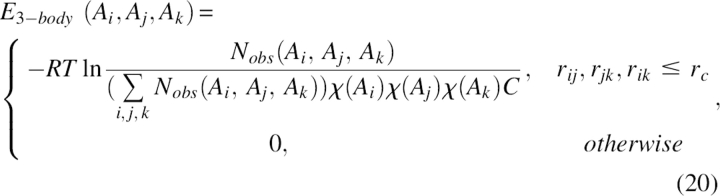 |
where Nobs(Ai, Aj, Ak) was the number of triplets of type (Ai, Aj, Ak) extracted from the database, and χ(Ai) was the mole fraction of the residue type Ai. C was a factor defined as:
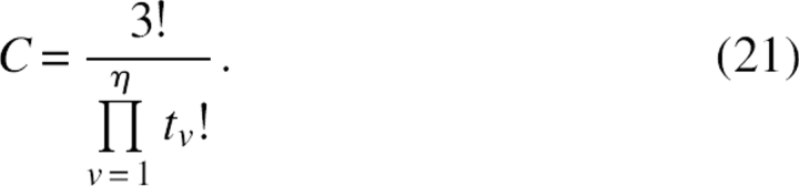 |
Here, η was the number of distinct residue types in the triplet (1 ≤ η ≤ 3), and tv was the number of residues of type v in the triplet.
Solvation energy based on the solvent-accessible surface
The term Esolvation was for the solvation energy based on the solvent-accessible surface (SAS). It was developed via statistical analysis of the side chain solvent-accessible surface in the nonhomologous structure database based on the all-atom structure model. For the Cα model, an approximate method for calculating the side chain SAS was developed, and the solvation energy was evaluated accordingly.
An approximate method was developed to calculate the side chain SAS from Cα atoms. Here, rres(i) was defined as the effective radius of the whole residue i, and SSC(i) was defined as the effective total solvent-accessible surface for the side chain of residue i. SSC(i) could be expressed by 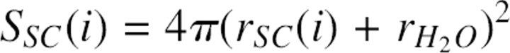 ; rSC(i) was the effective radius for the side chain of residue i, and
  was the radius of a water molecule (set to 1.4 Å). Also, dSC(i) was defined as the distance between the Cα atom and effective side chain center of residue i, and the positional vector of the side chain center was defined as R SC(i). It was assumed that the effective side chain center was always along the Cα to Cβ direction (Fig. 10). So,
 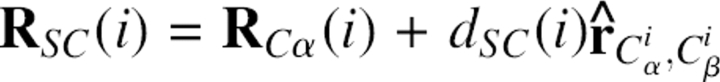 , where R Cα(i) was the Cα positional vector of residue i, and
  was the unit vector along the Cα to Cβ direction. The side chain SAS for residue i could then be calculated by:
Figure 10.

Schematic illustration of the parameters of the side-chain SAS from the Cα position. For residue i, rres(i) is the effective radius of the whole residue, rSC(i) is the effective radius for the side chain, dSC(i) is the distance between the Cα atom and effective side chain center, and R SC(i) is the positional vector of the side chain center. is the radius of a water molecule (1.4 Å).
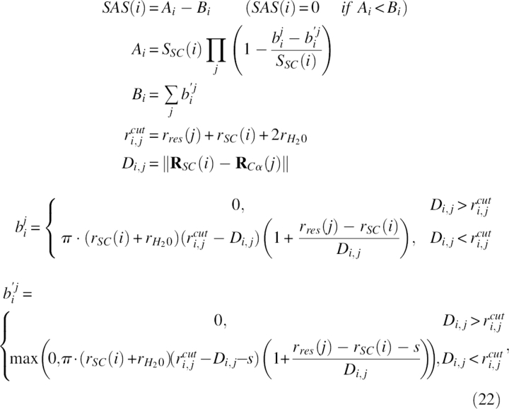 |
where s = 2.5 Å according to the literature (Wodak and Janin 1980). Here, there were 20 of rres(i), 19 of SSC(i), and 19 of dSC(i) as all the parameters in the SAS calculation.
In order to obtain the side chain SAS accurately for the coarse-grained model, all 58 parameters were trained against the atomic side chain SAS. The atomic side chain SAS was calculated based on look-up table methods (Bystroff 2002) and they were regarded as expected values. Then, a simulated annealing Monte Carlo simulation was used to optimize parameters according to the following target function on a set of 392 protein chains, which were selected from the nonhomologous structure database whose total number of residues range from 60 to 150 and there were no chain break, heteroatoms,, and missing atoms. The target function was:
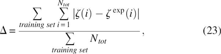 |
where Ntot was the total number of residues of a protein chain, and ζ(i), ζ exp(i) were the coarse-grained and expected fraction of solvent-accessible surface, respectively, which can be defined as the ratio between the side chain solvent-accessible surface and the total side chain surface area of that residue in isolation with the same configuration; i.e.,
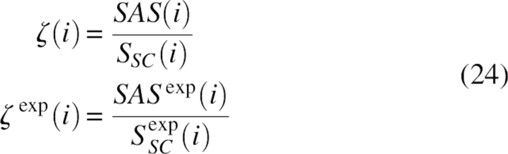 |
The optimized parameters can be found in Table 4, and the best target function value after optimization was 0.0917, indicating the existence of small error.
Table 4.
Values of 58 optimized parameters for determining the SAS of side chains

Finally, the energy term was related to the fraction of solvent-accessible surface ζ, which had a value between [0,1], and was uniformly divided into nbins = 20 bins. It was given by
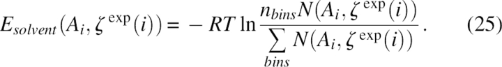 |
Here, Ai was the residue type of the target residue, and N(Ai, ζ exp (i)) was the observed number of occurrences of residue type Ai. When using the solvent energy term, ζ from the coarse-grained side chain SAS was used as the approximation of atomic value.
Weight optimization
Weights were optimized against all proteins in the LKF and Decoys'R'Us decoy set collections. To ease the decoy set dependence of weight optimization, these decoy sets were regrouped into three subsets based on the literature: The first subset consisted of 25 proteins in the Decoys'R'Us sets (Tobi and Elber 2000) (Subset-1 in Table 2), the second group consisted of 151 proteins in the LKF set (Loose et al. 2004; Zhang et al. 2006) (Subset-2 in Table 2), the third group consisted of the remaining 34 proteins in the LKF set and seven proteins in the Decoys'R'Us sets (Subset-3 in Table 2). The seven proteins from Decoys'R'Us in Subset-3 were 3icb in the 4state_reduced decoy set, 4icb in the fisa decoy set, 1eh2 and smd3 in the fisa_casp3 decoy set, 1beo and 4icb in the lattice_ssfit decoy set, and 4pti in the lmds decoy set.
In this study, an iterative protocol of Monte Carlo-simulated annealing was used on the three subsets of decoy collections. The cost function for optimization was:
where  was the average Z-score for all proteins in the group and N missing was the number of proteins whose native structures failed to be ranked first in energy. The Z-score of the native structure was defined as:
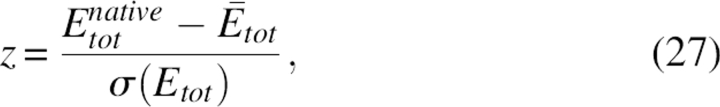 |
where Etotnative and Etot were the energy of the native and decoy structures for a particular protein, respectively,  and σ(Etot) were the average and standard deviation of energy of all decoys for a particular protein. The temperature factor kBT in the Monte Carlo simulation was decreased gradually during simulated annealing from 1.0 to 0.01 in 19,800 steps. Then, kBT was set to zero in Metropolis sampling, and the scoring function in Equation 26 was minimized for another 200 steps. The simulation started with predefined initial weights. Then, a randomly selected weight was increased or decreased by 0.1 in each Monte Carlo move, if the weight was within the predefined allowed range (see below for more details).
In detail, simulated annealing optimization was first performed on a randomly picked decoy subset with randomly assigned weights to obtain a set of optimized weights. Then, those weights were set as the new initial values for another round of simulated annealing optimization on a different decoy subset picked randomly. Optimizations were repeated among three decoy subsets 100 times. To make the simulation converge, the percentage changes of each weight with respect to the initial weight were restricted. In each round of simulation, the allowed percentage changes gradually decreased from 300% to a minimal 20%. However, to prevent the weights from being trapped at zero, the absolute allowed changes were no less than 0.5. According to weight optimization, weights finally converged. But the overall performance was not necessarily the best for the weight in the last step of annealing. So, we selected the best performing weights from the last few annealing steps.
Acknowledgments
M.C. and M.L. are partially supported by a predoctoral fellowship from the W.M. Keck Foundation of the Gulf Coast Consortia through the Keck Center for Computational and Structural Biology. Y.W. is partially supported by a grant from the Doer Foundation. J.M. acknowledges support from a grant from the National Institutes of Health (R01-GM067801).
Footnotes
Reprint requests to: Jianpeng Ma, One Baylor Plaza, BCM-125, Baylor College of Medicine, Houston, TX 77030, USA; e-mail: jpma@bcm.tmc.edu; fax: (713) 796-9438.
Article and publication are at http://www.proteinscience.org/cgi/doi/10.1110/ps.072796107.
References
- Adamian L. and Liang, J. 2001. Helix–helix packing and interfacial pairwise interactions of residues in membrane proteins. J. Mol. Biol. 311: 891–907. [DOI] [PubMed] [Google Scholar]
- Andrew C.D., Penel, S., Jones, G.R., and Doig, A.J. 2001. Stabilizing nonpolar/polar side-chain interactions in the α-helix. Proteins 45: 449–455. [DOI] [PubMed] [Google Scholar]
- Bahar I. and Jernigan, R.L. 1997. Inter-residue potentials in globular proteins and the dominance of highly specific hydrophilic interactions at close separation. J. Mol. Biol. 266: 195–214. [DOI] [PubMed] [Google Scholar]
- Betancourt M.R. and Thirumalai, D. 1999. Pair potentials for protein folding: Choice of reference states and sensitivity of predicted native states to variations in the interaction schemes. Protein Sci. 8: 361–369. [DOI] [PMC free article] [PubMed] [Google Scholar]
- Buchete N.V., Straub, J.E., and Thirumalai, D. 2004a. Development of novel statistical potentials for protein fold recognition. Curr. Opin. Struct. Biol. 14: 225–232. [DOI] [PubMed] [Google Scholar]
- Buchete N.V., Straub, J.E., and Thirumalai, D. 2004b. Orientational potentials extracted from protein structures improve native fold recognition. Protein Sci. 13: 862–874. [DOI] [PMC free article] [PubMed] [Google Scholar]
- Bystroff C. 2002. MASKER: Improved solvent-excluded molecular surface area estimations using Boolean masks. Protein Eng. 15: 959–965. [DOI] [PubMed] [Google Scholar]
- Colubri A., Jha, A.K., Shen, M.Y., Sali, A., Berry, R.S., Sosnick, T.R., and Freed, K.F. 2006. Minimalist representations and the importance of nearest neighbor effects in protein folding simulations. J. Mol. Biol. 363: 835–857. [DOI] [PubMed] [Google Scholar]
- DeBolt S.E. and Skolnick, J. 1996. Evaluation of atomic level mean force potentials via inverse folding and inverse refinement of protein structures: Atomic burial position and pairwise non-bonded interactions. Protein Eng. 9: 637–655. [DOI] [PubMed] [Google Scholar]
- Dehouck Y., Gilis, D., and Rooman, M. 2006. A new generation of statistical potentials for proteins. Biophys. J. 90: 4010–4017. [DOI] [PMC free article] [PubMed] [Google Scholar]
- Dobson C.M. and Karplus, M. 1999. The fundamentals of protein folding: Bringing together theory and experiment. Curr. Opin. Struct. Biol. 9: 92–101. [DOI] [PubMed] [Google Scholar]
- Dong Q., Wang, X., and Lin, L. 2006. Novel knowledge-based mean force potential at the profile level. BMC Bioinformatics 7: 324. [DOI] [PMC free article] [PubMed] [Google Scholar]
- Eisenberg D., Luthy, R., and Bowie, J.U. 1997. VERIFY3D: Assessment of protein models with three-dimensional profiles. Methods Enzymol. 277: 396–404. [DOI] [PubMed] [Google Scholar]
- Fabiola F., Bertram, R., Korostelev, A., and Chapman, M.S. 2002. An improved hydrogen bond potential: Impact on medium resolution protein structures. Protein Sci. 11: 1415–1423. [DOI] [PMC free article] [PubMed] [Google Scholar]
- Feng Y., Kloczkowski, A., and Jernigan, R.L. 2007. Four-body contact potentials derived from two protein datasets to discriminate native structures from decoys. Proteins doi: 10.1002/prot.21362. [DOI] [PubMed]
- Fidelis K., Stern, P.S., Bacon, D., and Moult, J. 1994. Comparison of systematic search and database methods for constructing segments of protein structure. Protein Eng. 7: 953–960. [DOI] [PubMed] [Google Scholar]
- Gatchell D.W., Dennis, S., and Vajda, S. 2000. Discrimination of near-native protein structures from misfolded models by empirical free energy functions. Proteins 41: 518–534. [PubMed] [Google Scholar]
- Godzik A., Kolinski, A., and Skolnick, J. 1995. Are proteins ideal mixtures of amino acids? Analysis of energy parameter sets. Protein Sci. 4: 2107–2117. [DOI] [PMC free article] [PubMed] [Google Scholar]
- Gohlke H. and Klebe, G. 2001. Statistical potentials and scoring functions applied to protein–ligand binding. Curr. Opin. Struct. Biol. 11: 231–235. [DOI] [PubMed] [Google Scholar]
- Hendlich M., Lackner, P., Weitckus, S., Floeckner, H., Froschauer, R., Gottsbacher, K., Casari, G., and Sippl, M.J. 1990. Identification of native protein folds amongst a large number of incorrect models. The calculation of low energy conformations from potentials of mean force. J. Mol. Biol. 216: 167–180. [DOI] [PubMed] [Google Scholar]
- Hinds D.A. and Levitt, M. 1992. A lattice model for protein structure prediction at low resolution. Proc. Natl. Acad. Sci. 89: 2536–2540. [DOI] [PMC free article] [PubMed] [Google Scholar]
- Hubner I.A., Deeds, E.J., and Shakhnovich, E.I. 2005. High-resolution protein folding with a transferable potential. Proc. Natl. Acad. Sci. 102: 18914–18919. [DOI] [PMC free article] [PubMed] [Google Scholar]
- Hutchinson E.G., Sessions, R.B., Thornton, J.M., and Woolfson, D.N. 1998. Determinants of strand register in antiparallel β-sheets of proteins. Protein Sci. 7: 2287–2300. [DOI] [PMC free article] [PubMed] [Google Scholar]
- Jernigan R.L. and Bahar, I. 1996. Structure-derived potentials and protein simulations. Curr. Opin. Struct. Biol. 6: 195–209. [DOI] [PubMed] [Google Scholar]
- Jones D.T., Taylor, W.R., and Thornton, J.M. 1992. A new approach to protein fold recognition. Nature 358: 86–89. [DOI] [PubMed] [Google Scholar]
- Kabsch W. and Sander, C. 1983. Dictionary of protein secondary structure—Pattern-recognition of hydrogen-bonded and geometrical features. Biopolymers 22: 2577–2637. [DOI] [PubMed] [Google Scholar]
- Keasar C. and Levitt, M. 2003. A novel approach to decoy set generation: Designing a physical energy function having local minima with native structure characteristics. J. Mol. Biol. 329: 159–174. [DOI] [PMC free article] [PubMed] [Google Scholar]
- Lazaridis T. and Karplus, M. 2000. Effective energy functions for protein structure prediction. Curr. Opin. Struct. Biol. 10: 139–145. [DOI] [PubMed] [Google Scholar]
- Liwo A., Lee, J., Ripoll, D.R., Pillardy, J., and Scheraga, H.A. 1999. Protein structure prediction by global optimization of a potential energy function. Proc. Natl. Acad. Sci. 96: 5482–5485. [DOI] [PMC free article] [PubMed] [Google Scholar]
- Loose C., Klepeis, J.L., and Floudas, C.A. 2004. A new pairwise folding potential based on improved decoy generation and side-chain packing. Proteins 54: 303–314. [DOI] [PubMed] [Google Scholar]
- Lu H. and Skolnick, J. 2001. A distance-dependent atomic knowledge-based potential for improved protein structure selection. Proteins 44: 223–232. [DOI] [PubMed] [Google Scholar]
- MacKerell A.D., Bashford Jr, D., Bellott, M., Dunbrack Jr, R.L., Evanseck, J.D., Field, M.J., Fischer, S., Gao, J., Guo, H., Ha, S., et al. 1998. All-atom empirical potential for molecular modeling and dynamics studies of proteins. J. Phys. Chem. B102: 3586–3616. [DOI] [PubMed] [Google Scholar]
- McConkey B.J., Sobolev, V., and Edelman, M. 2003. Discrimination of native protein structures using atom–atom contact scoring. Proc. Natl. Acad. Sci. 100: 3215–3220. [DOI] [PMC free article] [PubMed] [Google Scholar]
- Meller J. and Elber, R. 2002. Protein recognition by sequence-to-structure fitness: Bridging efficiency and capacity of threading models. Adv. Chem. Phys. 120: 77–130. [Google Scholar]
- Melo F. and Feytmans, E. 1998. Assessing protein structures with a non-local atomic interaction energy. J. Mol. Biol. 277: 1141–1152. [DOI] [PubMed] [Google Scholar]
- Melo F., Sanchez, R., and Sali, A. 2002. Statistical potentials for fold assessment. Protein Sci. 11: 430–448. [DOI] [PMC free article] [PubMed] [Google Scholar]
- Milik M., Kolinski, A., and Skolnick, J. 1997. Algorithm for rapid reconstruction of protein backbone from α carbon coordinates. J. Comput. Chem. 18: 80–85. [Google Scholar]
- Miyazawa S. and Jernigan, R.L. 1985. Estimation of effective interresidue contact energies from protein crystal-structures—Quasi-chemical approximation. Macromolecules 18: 534–552. [Google Scholar]
- Miyazawa S. and Jernigan, R.L. 1996. Residue–residue potentials with a favorable contact pair term and an unfavorable high packing density term, for simulation and threading. J. Mol. Biol. 256: 623–644. [DOI] [PubMed] [Google Scholar]
- Miyazawa S. and Jernigan, R.L. 2005. How effective for fold recognition is a potential of mean force that includes relative orientations between contacting residues in proteins? J. Chem. Phys. doi: 10.1063/1.1824012. [DOI] [PubMed]
- Moult J. 1997. Comparison of database potentials and molecular mechanics force fields. Curr. Opin. Struct. Biol. 7: 194–199. [DOI] [PubMed] [Google Scholar]
- Park B. and Levitt, M. 1996. Energy functions that discriminate X-ray and near native folds from well-constructed decoys. J. Mol. Biol. 258: 367–392. [DOI] [PubMed] [Google Scholar]
- Poole A.M. and Ranganathan, R. 2006. Knowledge-based potentials in protein design. Curr. Opin. Struct. Biol. 16: 508–513. [DOI] [PubMed] [Google Scholar]
- Qiu J. and Elber, R. 2005. Atomically detailed potentials to recognize native and approximate protein structures. Proteins 61: 44–55. [DOI] [PubMed] [Google Scholar]
- Rajgaria R., McAllister, S.R., and Floudas, C.A. 2006. A novel high resolution Cα–Cα distance dependent force field based on a high quality decoy set. Proteins 65: 726–741. [DOI] [PubMed] [Google Scholar]
- Russ W.P. and Ranganathan, R. 2002. Knowledge-based potential functions in protein design. Curr. Opin. Struct. Biol. 12: 447–452. [DOI] [PubMed] [Google Scholar]
- Samudrala R. and Moult, J. 1998. An all-atom distance-dependent conditional probability discriminatory function for protein structure prediction. J. Mol. Biol. 275: 895–916. [DOI] [PubMed] [Google Scholar]
- Samudrala R., Xia, Y., Levitt, M., and Huang, E.S. 1999. A combined approach for ab initio construction of low resolution protein tertiary structures from sequence. Pacific Symposium on Biocomputing 4: 505–516. [DOI] [PubMed] [Google Scholar]
- Shen M.Y. and Sali, A. 2006. Statistical potential for assessment and prediction of protein structures. Protein Sci. 15: 2507–2524. [DOI] [PMC free article] [PubMed] [Google Scholar]
- Shi Z., Olson, C.A., and Kallenbach, N.R. 2002. Cation-π interaction in model α-helical peptides. J. Am. Chem. Soc. 124: 3284–3291. [DOI] [PubMed] [Google Scholar]
- Simons K.T., Kooperberg, C., Huang, E., and Baker, D. 1997. Assembly of protein tertiary structures from fragments with similar local sequences using simulated annealing and Bayesian scoring functions. J. Mol. Biol. 268: 209–225. [DOI] [PubMed] [Google Scholar]
- Simons K.T., Ruczinski, I., Kooperberg, C., Fox, B.A., Bystroff, C., and Baker, D. 1999. Improved recognition of native-like protein structures using a combination of sequence-dependent and sequence-independent features of proteins. Proteins 34: 82–95. [DOI] [PubMed] [Google Scholar]
- Sippl M.J. 1990. Calculation of conformational ensembles from potentials of mean force. An approach to the knowledge-based prediction of local structures in globular proteins. J. Mol. Biol. 213: 859–883. [DOI] [PubMed] [Google Scholar]
- Sippl M.J. 1995. Knowledge-based potentials for proteins. Curr. Opin. Struct. Biol. 5: 229–235. [DOI] [PubMed] [Google Scholar]
- Skolnick J. 2006. In quest of an empirical potential for protein structure prediction. Curr. Opin. Struct. Biol. 16: 166–171. [DOI] [PubMed] [Google Scholar]
- Stapley B.J. and Doig, A.J. 1997. Hydrogen bonding interactions between glutamine and asparagine in α-helical peptides. J. Mol. Biol. 272: 465–473. [DOI] [PubMed] [Google Scholar]
- Steward R.E. and Thornton, J.M. 2002. Prediction of strand pairing in antiparallel and parallel β-sheets using information theory. Proteins 48: 178–191. [DOI] [PubMed] [Google Scholar]
- Tanaka S. and Scheraga, H.A. 1976. Medium- and long-range interaction parameters between amino acids for predicting three-dimensional structures of proteins. Macromolecules 9: 945–950. [DOI] [PubMed] [Google Scholar]
- Thomas P.D. and Dill, K.A. 1996. Statistical potentials extracted from protein structures: How accurate are they? J. Mol. Biol. 257: 457–469. [DOI] [PubMed] [Google Scholar]
- Tobi D. and Elber, R. 2000. Distance-dependent, pair potential for protein folding: Results from linear optimization. Proteins 41: 40–46. [PubMed] [Google Scholar]
- Wang G. and Dunbrack Jr, R.L. 2003. PISCES: A protein sequence culling server. Bioinformatics 19: 1589–1591. [DOI] [PubMed] [Google Scholar]
- Wodak S.J. and Janin, J. 1980. Analytical approximation to the accessible surface-area of proteins. Proc. Natl. Acad. Sci. USA 77: 1736–1740. [DOI] [PMC free article] [PubMed] [Google Scholar]
- Wu Y., Chen, M., Lu, M., Wang, Q., and Ma, J. 2005a. Determining protein topology from skeletons of secondary structures. J. Mol. Biol. 350: 571–586. [DOI] [PubMed] [Google Scholar]
- Wu Y., Tian, X., Lu, M., Chen, M., Wang, Q., and Ma, J. 2005b. Folding of small helical proteins assisted by small-angle X-ray scattering profiles. Structure 13: 1587–1597. [DOI] [PubMed] [Google Scholar]
- Xia Y., Huang, E.S., Levitt, M., and Samudrala, R. 2000. Ab initio construction of protein tertiary structures using a hierarchical approach. J. Mol. Biol. 300: 171–185. [DOI] [PubMed] [Google Scholar]
- Zhang C., Vasmatzis, G., Cornette, J.L., and DeLisi, C. 1997. Determination of atomic desolvation energies from the structures of crystallized proteins. J. Mol. Biol. 267: 707–726. [DOI] [PubMed] [Google Scholar]
- Zhang Y., Kolinski, A., and Skolnick, J. 2003. TOUCHSTONE II: A new approach to ab initio protein structure prediction. Biophys. J. 85: 1145–1164. [DOI] [PMC free article] [PubMed] [Google Scholar]
- Zhang C., Liu, S., Zhou, H., and Zhou, Y. 2004. An accurate, residue-level, pair potential of mean force for folding and binding based on the distance-scaled, ideal-gas reference state. Protein Sci. 13: 400–411. [DOI] [PMC free article] [PubMed] [Google Scholar]
- Zhang J., Chen, R., and Liang, J. 2006. Empirical potential function for simplified protein models: Combining contact and local sequence-structure descriptors. Proteins 63: 949–960. [DOI] [PubMed] [Google Scholar]
- Zhou H. and Zhou, Y. 2002. Distance-scaled, finite ideal-gas reference state improves structure-derived potentials of mean force for structure selection and stability prediction. Protein Sci. 11: 2714–2726. [DOI] [PMC free article] [PubMed] [Google Scholar]
- Zhou Y., Zhou, H., Zhang, C., and Liu, S. 2006. What is a desirable statistical energy function for proteins and how can it be obtained? Cell Biochem. Biophys. 46: 165–174. [DOI] [PubMed] [Google Scholar]