

Abstract
Retinotopy is a fundamental organizing principle of the visual cortex. Over the years, a variety of techniques have been used to examine it. None of these techniques, however, provides a way to rapidly characterize retinotopy, at the submillimeter range, in alert, behaving subjects. Voltage-sensitive dye imaging (VSDI) can be used to monitor neuronal population activity at high spatial and temporal resolutions. Here we present a VSDI protocol for rapid and precise retinotopic mapping in the behaving monkey. Two monkeys performed a fixation task while thin visual stimuli swept periodically at a high speed in one of two possible directions through a small region of visual space. Because visual space is represented systematically across the cortical surface, each moving stimulus produced a traveling wave of activity in the cortex that could be precisely measured with VSDI. The time at which the peak of the traveling wave reached each location in the cortex linked this location with its retinotopic representation. We obtained detailed retinotopic maps from a region of about 1 cm2 over the dorsal portion of areas V1 and V2. Retinotopy obtained during <4 min of imaging had a spatial precision of 0.11–0.19 mm, was consistent across experiments, and reliably predicted the locations of the response to small localized stimuli. The ability to rapidly obtain precise retinotopic maps in behaving monkeys opens the door for detailed analysis of the relationship between spatiotemporal dynamics of population responses in the visual cortex and perceptually guided behavior.
INTRODUCTION
Topography—the orderly representation of sensory and motor information—is a fundamental feature of many sensory and motor cortical areas (e.g., Hubel and Weisel 1977; Knudsen et al. 1987; Woolsey 1952). In a topographic map, neurons that share response properties are clustered together into columns that extend radially from the pial surface to the white matter (Hubel and Weisel 1963; Mountcastle 1957). Neurons in nearby locations along the cortical surface represent similar sensory or motor parameters, forming a systematic map of those parameters.
A visual cortical area is considered retinotopically or visuotopically organized if nearby locations within this area represent nearby locations in visual space. In primates, the striate cortex (V1) and many extrastriate visual cortical areas including the secondary visual area (V2) are retinotopically organized (for review, see Gattass et al. 2005; Polimeni et al. 2006). The retinotopic organization of primate V1 and V2 has been studied extensively using a variety of experimental approaches, including lesions studies (e.g., Glickstein and Whitteridge 1987; Holmes 1945; Horton and Hoyt 1991), electrophysiological recordings (e.g., Allman and Kaas 1974; Daniel and Witteridge 1961; Hubel and Wiesel 1974; Talbot and Marshall 1941; Van Essen and Zeki 1978; Van Essen et al. 1984), 2-deoxyglucose autoradiography (Tootell et al. 1982, 1988), cytochrome oxidase staining of the representation of angioscotomas (Adams and Horton 2003), electrical stimulation (e.g., Bradley et al. 2005; Dobelle et al. 1979), positron emission tomography (Fox et al. 1987), functional magnetic resonance imaging (fMRI) (e.g., Brewer et al. 2002; DeYoe et al. 1996; Engel et al. 1994, 1997; Fize et al. 2003; Larsson and Heeger 2006; Sereno et al. 1995; Wandell et al. 2005), and optical imaging of intrinsic signals (Blasdel and Campbell 2001). None of these techniques, however, allows for rapid and precise retinotopic mapping of the cortex at the submillimeter range in alert, behaving subjects.
Optical imaging with voltage-sensitive dyes provides a method for directly measuring changes in electrical activity of populations of neurons (for review, see Grinvald and Hildesheim 2004) and can be used to monitor neural population responses in the cortex of alert, behaving monkeys (Chen et al. 2006; Seidemann et al. 2002; Slovin et al. 2002). Because changes in membrane potentials are converted by the dye molecules into changes in fluorescence within microseconds (Grinvald et al. 1999), VSDI is a particularly powerful tool for studying the dynamics of neural population responses to moving stimuli (e.g., Jancke et al. 2004).
Here we report the first use of VSDI to obtain high-precision retinotopic maps from V1 and V2 of two alert, behaving monkeys. To measure retinotopy, we combined VSDI in the behaving monkey with phase-encoding techniques in which the phase of the response to a periodic moving stimulus is used to obtain the retinotopic coordinate at each location. Phase-encoding techniques have been used to map the visual cortex of humans using fMRI (e.g., DeYoe et al. 1996; Engel et al. 1994, 1997; Sereno et al. 1995). More recently, these techniques have been adopted to map the visual cortex of the anesthetized mouse and cat using optical imaging of intrinsic signals (Kalatsky and Stryker 2003). We now demonstrate that retinotopic maps that are obtained within minutes of VSDI imaging have high precision (<0.2 mm), are highly reproducible across experiments, and can be used to predict the location of the response to small localized visual stimuli.
METHODS
Two macaque monkeys were used in this study. Our general experimental techniques have been described in detail elsewhere (Arieli et al. 2002; Chen et al. 2006; Grinvald et al. 1999; Seidemann et al. 2002; Slovin et al. 2002). We subsequently focus on details that are specific to the current study. All procedures were approved by the University of Texas Institutional Animal Care and Use Committee and conformed to National Institutes of Health standards.
Visual stimulus
Visual stimuli were presented on a 21-in. color display extending over 20.5 × 15.4° at a viewing distance of 108 cm. The display had pixel resolution of 1,024 × 768 (50 pixels/deg) and a refresh rate of 100 Hz.
STIMULI FOR RETINOTOPIC MAPPING
We used two types of visual stimuli for the detailed retinotopic mapping. To map polar angle, we used a short segment of a thin radial wedge stimulus (2.88° of visual angle long) that moved from the contralateral side (relative to the mapped hemisphere) toward the lower vertical meridian (counterclockwise direction in Fig. 1D because, in this case, imaging was from the right hemisphere) over a distance of 60 angular degrees at 45 angular degrees off the vertical. To map eccentricity, we used a short segment of a thin ring (60 angular degrees long) that moved inward toward the fovea over a distance of 2.88° of visual angle starting at eccentricity of 4.2° (Fig. 1E). In all cases, as the stimulus moved it covered exactly the same area in visual space that was approximately a trapezoidal aperture in the lower visual field. The two stimuli started and ended their movement well outside the mapped region of cortex to avoid possible artifacts arising from the transient onset and offset of the stimulus.
FIG. 1.
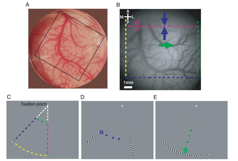
Imaging area, visual stimulus, and coarse retinotopy. A: imaging chamber over the dorsal portion of primary visual cortex (V1) and secondary visual cortex (V2) in the right hemisphere. A typical imaging area of 14 × 14 mm is indicated by the black square. B: image of the cortical vasculature taken through the imaging camera in one of the retinotopic mapping experiments. Four colored dashed lines delineate roughly the cortical representation of the stimulus in C. Magenta line indicates the V1/V2 border. Arrows indicate the directions that correspond to the directions of motion of the stimuli shown in D and E. Scale bar in this and all other figures is 1 mm. C: mapped region of visual space. Four colored dashed lines correspond roughly to those in B. D: radial wedge stimulus moving in the counterclockwise direction. E: ring segment stimulus moving in the inward direction.
On each trial, the stimulus appeared at one of the sides of the trapezoidal aperture and moved in equal steps until it reached the opposite side after 24 video frames. After the 24th video frame, the stimulus returned to its starting position and repeated the same trajectory for a total of seven cycles. The period of each sweep was therefore 24 video frames (240 ms).
Stimulation at this temporal frequency provided excellent signal-to-noise ratios because the power spectrum of the noise at this frequency was relatively low compared with lower frequencies and because multiple cycles were acquired in a relatively short imaging interval. Short imaging intervals were advantageous because they limited bleaching of the dye and possible photodynamic damage to the tissue (Grinvald et al. 1999) and because they allowed more precise synchronization to the monkey’s heart beat (Grinvald et al. 1999).
We used two possible stimulus configurations for the moving stimuli. In the first configuration the stimulus moved on every video frame in 24 equal steps and had a width of 1/24 of the length of its trajectory (wedge width, 2.5 angular degrees; ring width, 0.12° of visual angle). In the second configuration, the same stimulus was displayed for two consecutive frames (effective refresh rate of 50 Hz). In this case, the stimulus moved in 12 equal steps and had a width of 1/12 of the length of its trajectory (wedge width, 5 angular degrees; ring width, 0.24° of visual angle). We did not observe significant differences between these two types of stimuli (see Fig. 5, C and D for direct comparison between the retinotopic maps obtained by these two configurations).
FIG. 5.
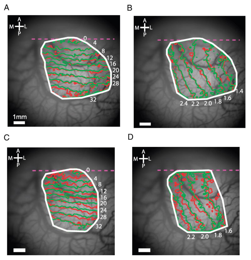
Reproducibility of retinotopic maps. A: polar maps obtained separately for 18 odd and 18 even trials. B: eccentricity maps obtained separately from 18 odd and 18 even trials. C: polar map from a second experiment with 10 repetitions (red curves) aligned with the polar map from the first experiment (green curves) based on the cortical vasculature. D: eccentricity maps from the 2 experiments aligned based on the cortical vasculature.
On each frame, the stimulus (wedge or ring segment) was a thin slice of a fixed spiral grating oriented at 45° relative to radial (100% contrast, 16 cycles/deg at the most foveal location, and 5.2 cycles/deg at the most peripheral location). Stimulus orientation was not varied in this study, but because stimulus speed and spatial frequencies were quite high, it seems unlikely that stimulus pattern orientation would affect the retinotopic maps. The stimulus was presented on a uniform gray background with the same mean luminance (24 cd/m2).
In a given experiment, each of the two possible stimuli was repeated 10–36 times together with the same number of trials with no visual stimulus (blank trials) in a pseudorandom order. A full block of trials took 5–15 min to complete, leaving plenty of time for other experimental conditions to be tested in the same recording session (typically ~3 h long).
SINGLE-FRAME STIMULUS
To confirm the retinotopy obtained using the moving stimuli, we also included a few conditions in which only a single frame from the movie was presented periodically. This stimulus had identical timing to the movies used in the retinotopic mapping with the exception that all frames but one were replaced with a uniform gray stimulus. For example, in one such stimulus, a wedge would appear for one video frame on the vertical meridian at the same time as in the counterclockwise movie, and then reappear at the same location after 24 video frames for a total of seven cycles.
To obtain the retinotopic representation of this single-frame stimulus, we first determined the region of cortex in which reliable modulations at the stimulus frequency could be measured (see following text). At each location within this region, we obtained the amplitude and phase of the modulation at the stimulus frequency using fast Fourier transform (FFT). The locations in the cortex with the shortest phase were considered the cortical representation of this stimulus. We then compared the locations with the shortest phase with the predicted locations based on the retinotopic maps.
Eye position monitoring
Eye position was monitored at 250 Hz using an infrared analog eye tracker (Dr. Bouis, Karlsruhe, Germany). The monkey was required to maintain fixation within a window (<2°) centered around the fixation point to receive a liquid reward. Trials in which the eyes strayed outside of the fixation window were immediately aborted and were followed by a time-out period. Only trials with successful fixation were further analyzed.
Imaging parameters and data analysis
We used an Imager 3001 system (Optical Imaging, Rehovot, Israel) to image brain activity. Each imaging trial lasted 2.1 s in which the camera collected 230 frames at 110 Hz. Each VSDI image frame had 512 × 512 pixels with a pixel size of approximately 0.03 × 0.03 mm.
PREPROCESSING
VSDI signals were first smoothed with Gaussian filters (σ = 0.055 mm in space and σ = 4.55 ms in time) to remove high-frequency spatial and temporal noise. The smoothed signals at each location were then normalized by the average fluorescence at that location across all trials and frames to remove the effects of uneven illumination and nonuniform staining. To remove a slow, roughly linear drift in the VSD signal, a linear regression was performed at each location on each trial and the fitted linear trend was removed from the dye signal. For each condition, the median dye signal across all trials at each time point was obtained and the medians for stimulus conditions minus the median for the blank condition were taken as the final VSDI responses. Subtracting the response in the blank condition served to remove systematic and repeatable artifacts that are common to all trials such as heartbeat artifacts. Finally, to remove any residual differences in the initial responses, the mean of the first seven imaging frames before stimulus presentation was subtracted from the VSDI responses.
DATA ANALYSIS
VSDI responses showed clear modulations at the stimulus frequency (see Figs. 2 and 3). To minimize the effect of the transients at stimulus onset and offset, the first and the last cycles of the response were excluded from the quantitative analysis of response phase. The interval over which VSDI responses were analyzed is indicated by the vertical lines in Fig. 2B. Response phase was estimated from the responses at each location using FFT.
FIG. 2.
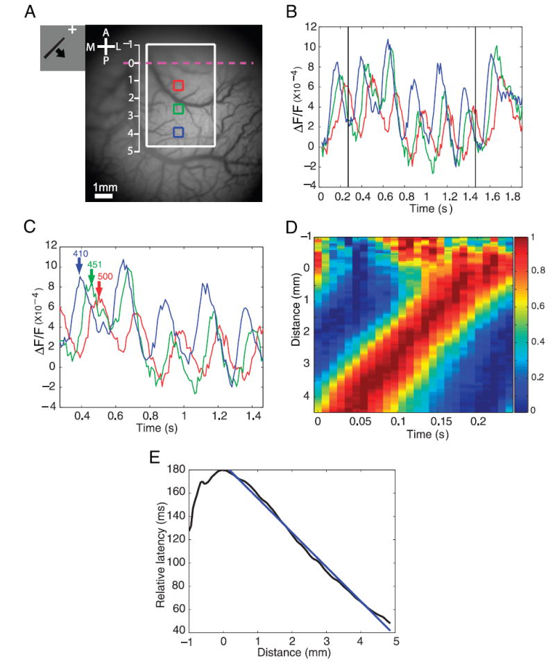
Cortical wave of activity in response to a radial wedge moving in the counterclockwise direction. A: image of cortical vasculature. Imaging area of about 10 × 10 mm. White rectangle, subregion (4.14 × 6.07 mm) used for the analysis in D and E. Vertical scale, distances measured in millimeters from the V1/V2 border. B: time course of voltage-sensitive dye imaging (VSDI) response at 3 selected locations (colored squares in A). Squares had a size of 0.607 × 0.607 mm and their centers were 1.38 mm apart. C: time courses in the middle 5 cycles. Here and in Fig. 3C, fast Fourier transform (FFT) was performed on the 5 middle cycles to obtain the phase from which the time-to-peak of the response relative to stimulus onset (inset numbers in milliseconds are time-to-second peak) was derived (see METHODS). D: space–time color plot of normalized average time courses within the white rectangle as a function of the distance from the V1/V2 border. Time courses at each location were averaged across the 5 cycles, then averaged across the horizontal (lateral–medial) spatial dimension, and finally normalized to [0, 1]. E: relative time-to-peak vs. distance from V1/V2 border, identified by the reversal in the polar angle component of the retinotopic map, i.e., as the strip of cortex with longest latency. Time-to-peak at the V1/V2 border (vertical meridian) was set to 180 ms, the time it took for the stimulus to travel from its initial position at 225 ° to the vertical meridian in the first cycle. All other latencies shown here and in Fig. 3E were specified relative to the lower vertical meridian such that they represent only the delay arising from the time it took the visual stimulus to reach the neurons’ receptive fields (see METHODS). Straight blue line is a linear fit to the latency–distance relation in the region of interest (ROI).
FIG. 3.
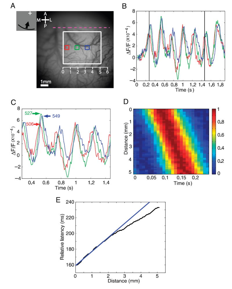
Cortical wave of activity in response to a ring segment moving inward. A: image of cortical vasculature. Imaging area of about 10 × 10 mm. White rectangle, subregion (5.24 × 4.42 mm) used for the analysis in D and E. Horizontal scale, distances measured in millimeters from the most medial portion of the white rectangle. B: time course of VSDI response at 3 selected locations (colored squares in A). Squares had a size of 0.607 × 0.607 mm and their centers were 1.38 mm apart. C: time courses in the middle 5 cycles. D: space–time color plot of normalized time courses as a function of the distance from the most medial point within the white square. Time courses at each location were averaged across the 5 cycles, then averaged across the vertical (anterior–posterior) spatial dimension, and finally normalized to the range [0, 1]. E: time-to-peak vs. distance from the medial edge of the white rectangle. Straight blue line is a linear fit to part of the latency–distance relation in the ROI.
The time it takes for the response to a moving stimulus to reach its peak at location i, ti, is the sum of two components: 1) a fixed delay l attributed to the neural latency of the response (i.e., the time it takes the response to a stimulus that directly activates the receptive field of the neurons at this cortical location to reach its peak) and 2) a variable delay that depends on the time it takes the moving stimulus to reach the receptive field of the neurons at the selected location. Thus ti = l + (di/s), where di is the distance between the retinotopic coordinate at location i and the initial location of the stimulus (e.g., 225 angular deg for the wedge moving in the counterclockwise direction) and s is the speed of the stimulus (e.g., 60 angular deg per 240 ms).
A polar wedge moving toward the lower vertical meridian triggered two waves of activity in V1 and V2 that moved toward each other. These waves met at the V1/V2 border (Fig. 2, D and E). By assuming that the location where the two cortical waves met represents the vertical meridian, an assumption that we subsequently verify (Fig. 6A), we obtained the fixed-latency component as the time-to-peak at the V1/V2 border minus 180 ms (the time it took the wedge to reach the vertical meridian). By further assuming that the fixed latency was constant within our region of interest (ROI) (an assumption that is subsequently confirmed), we directly obtained the retinotopic coordinate at each location i by computing its distance from the initial position as di = (ti − l)s and adding this value to the initial position of the stimulus.
FIG. 6.
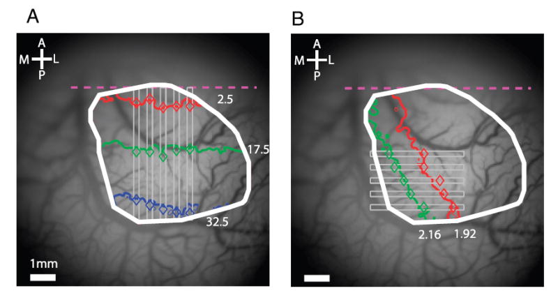
Predicted vs. observed locations of responses to thin wedges and ring segments. A: polar angle component of retinotopic map. Diamonds, observed locations corresponding to thin wedges (5 deg of polar angle wide) presented at 2.5° (red), 17.5° (green), and 32.5° (blue) relative to the lower vertical meridian. These locations exhibited the shortest response latency in each of 5 vertical strips (thin gray rectangles, 0.276 mm wide, 0.552 mm apart). Colored lines, isopolar contours corresponding to the same locations in the visual field from the retinotopic map in Fig. 4B. B: radial component of the retinotopic map. Diamonds, observed locations corresponding to thin ring segments (0.24° of visual angle wide) presented at eccentricities of 1.92° (red) and 2.16° (green). These locations exhibited the shortest response latencies in each of 5 horizontal strips (thin gray rectangles, 0.276 mm wide, 0.552 mm apart) extending across the ROI (white rectangle). Colored lines, isoeccentricity contours from the retinotopic map in Fig. 4D. Times-to-peak were computed within each thin rectangular ROI by first averaging the signals along the narrow dimension of the ROI.
Quantitative analysis of retinotopy was restricted to an ROI that was selected based on two criteria: 1) the correlation between the stimuli and corresponding responses [the ratio of amplitude at stimulus frequency to the square root of the time-series power (Engel et al. 1997) was >0.5] and 2) the amplitude at stimulus frequency at the specific location was >50% of the maximal modulation amplitude across all locations. Convex, connected ROIs were cropped manually based on these criteria. The resulting ROIs were usually about 5 × 5 mm.
To assess the precision of our retinotopic measurements, a bootstrap sampling procedure was performed. A set of 28 trials was randomly selected with replacement from the 36 repetitions for each condition and the retinotopic coordinates at each location within the ROI were obtained based on this sample using the procedures described earlier. This procedure was repeated 500 times and a distribution of retinotopic coordinates at each location in the ROI was obtained. From this distribution, a 95% confidence interval on the retinotopic coordinates was obtained. In addition, we used this procedure to determine the distance in the cortex at which the overlap in the distributions of retinotopic coordinates was <5%.
To evaluate quantitatively the reproducibility (Fig. 5) and predictability (Fig. 6) of the retinotopy, we first computed at each cortical location the distance between the two retinotopic coordinates (e.g., the coordinates obtained in two separate experiments or in the same experiment using two different stimuli). Distance in the cortex was obtained by multiplying distance in retinotopic coordinates by the average cortical magnification factor (CMF) in the ROI.
Large curvature in the imaged area could lead to significant distortions in our retinotopic maps. The regions of interest analyzed here were restricted to relatively planar portions of the cortex. We estimated (based on the depth of field of the camera) that the differences in depth within these regions were less than 200 microns. Such small differences are likely to produce negligible distortions.
ALIGNMENT PROTOCOL
To compare maps obtained in different experimental sessions (on different days), we used an image-registration algorithm based on techniques adopted from the computer vision literature and modified from an algorithm used to align data from fMRI experiments (Nestares and Heeger 2000). Most image-registration techniques rely on the assumption that corresponding pixels in the two images have equal intensity, which is not true for optical imaging of the brain across experiment sessions because of differences in the geometric arrangement of the camera and lighting with respect to the cortical surface. Thus the images were preprocessed with intensity normalization and contrast equalization to minimize the differences between the intensities of the two images (for details, see Nestares and Heeger 2000). However, because these preprocessing steps did not correct perfectly for the image differences, the alignment algorithm relied on robust estimation (Beaton and Tukey 1974; Hampel et al. 1986; Holland and Welsch 1977) to automatically ignore pixels where the intensities were sufficiently different in the two images. The output of the registration algorithm was an affine transformation (rotation, translation, scaling in x and y, linear shear in x and y) that best matched (using the robust, not least-squares, metric) the intensity- and contrast-corrected images of the vasculature from the two experimental sessions. An implementation of this algorithm is available to download (http://earth.psy.utexas.edu/sourcecode/vsdAlign).
RESULTS
Experimental design
We used VSDI to obtain high-resolution retinotopic maps from two macaque monkeys. Retinotopic maps were obtained from a region of approximately 1 cm2 over the dorsal portion of areas V1 and V2 (Fig. 1, A and B). In the macaque, the dorsal border between V1 and V2 (dashed magenta line in Fig. 1B) runs roughly parallel to the lunate sulcus and is located a few millimeters posterior to it.
The coarse retinotopy in this portion of the macaque cortex is well established (e.g., Daniel and Witteridge 1961; Tootell et al. 1988; Van Essen et al. 1984) and is illustrated by the approximate mapping between the colored curves in Fig. 1C and their corresponding representation in V1 and V2 (colored lines in Fig. 1B). Specifically, neurons at the border between V1 and V2 represent the lower vertical meridian. As one moves outward from the fovea toward the periphery along the vertical meridian, the cortical representation shifts from lateral to medial along the V1/V2 border. Therefore the more foveal ring section (green curve, Fig. 1C) is represented by the more lateral vertical green line in V1 and V2 (Fig. 1B). The more peripheral ring section (yellow curve, Fig. 1C) is represented by the more medial yellow vertical line in V1 and V2 (Fig. 1B).
Polar angle representation in V1 and V2 is mirror symmetric relative to the V1/V2 border. As one changes the polar angle away from vertical toward the contralateral direction (clockwise direction because this is the right hemisphere), the cortical representation advances in the posterior direction in V1 and in the anterior direction in V2 but remains roughly parallel to the V1/V2 border. Because most of V2 is located in the posterior bank of the lunate sulcus, with only a small portion extending to the cortical surface posterior to the lunate, the representation of the blue bar in Fig. 1C is visible in V1 but not in V2.
The visual stimuli used in the current study were designed to take advantage of this known organization. The monkeys were trained to maintain gaze on a central fixation point. While the monkey maintained fixation, a thin radial wedge or a thin-ring segment with alternating light and dark stripes appeared at one side of an approximately trapezoidal aperture and swept rapidly toward the opposite side of the aperture (see METHODS).
To obtain a detailed retinotopic map of polar angle, a short radial wedge rotated periodically from the contralateral side toward the vertical meridian (counterclockwise direction in Fig. 1D). To obtain a detailed retinotopic map of eccentricity, a short ring segment moved periodically in the inward direction (Fig. 1E). Note that the two stimuli (polar and radial) spanned exactly the same region of visual space.
Given the coarse retinotopic organization in this region, each sweep of the wedge moving toward the lower vertical meridian was expected to trigger two simultaneous waves of cortical activity that would start far from the V1/V2 border and propagate toward the border in the anterior direction in V1 and in the posterior direction in V2 (blue arrows in Fig. 1B). These waves were expected to be oriented approximately parallel to the V1/V2 border. Similarly, each sweep of the ring segment moving inward was expected to trigger a wave of cortical activity that would start in the medial portion of V1 and V2 and propagate laterally (green arrow in Fig. 1B). As subsequently described in detail, we used the times at which these cortical waves reached each location in the cortex to obtain the corresponding retinotopic polar and eccentricity coordinates at that location.
Cortical waves in response to moving stimuli
While the monkey performed the fixation task, VSDI signals were measured from the visual cortex using the oxonol dyes RH-1691 or RH-1838 (Grinvald and Hildesheim 2004; Shoham et al. 1999). Figure 2B shows the average time course of the optical signal in three selected regions in V1 (colored squares in Fig. 2A) in response to the radial wedge moving in the counterclockwise direction. At all three regions, the VSD response rose up rapidly after stimulus onset and then continued to modulate at the stimulus frequency (4.166 Hz) for seven cycles.
The propagation of the cortical wave of activity that was triggered by a wedge moving in the counterclockwise direction can be observed by comparing the time courses of the response at different distances from the V1/V2 border. There were clear time lags between the time courses at the three selected regions (Fig. 2C). As expected, the response peaked first at the location further away from the V1/V2 border (blue curve), then at the middle location (green curve), and finally at the location closest to the V1/V2 border (red curve). The green trace was 41 ms delayed relative to the blue trace, and 49 ms ahead of the red trace. These time differences can be used to obtain the distance between the retinotopic representations at these three regions. Because the stimulus period was 240 ms and the distance traveled by the stimulus was 60 angular deg, these time differences correspond to a distance of 10.25 angular deg between the blue and green regions and a distance of 12.25 angular deg between the green and red regions.
As expected, a wedge moving in the counterclockwise direction triggered two waves of activity that started far from the V1/V2 border and moved toward it. To examine these waves in more detail, we computed the counterclockwise responses at each location in a rectangular ROI (white rectangle, Fig. 2A) and averaged the responses over space along the horizontal (medial–lateral) direction. We then averaged the responses across the middle five cycles, normalized the response, and plotted these time courses as a function of their distance from the V1/V2 border (Fig. 2D). The cortical wave was clearly evident in V1, starting far from the V1/V2 border (Fig. 2D, bottom left) and moving toward the border where it met a second wave that arrived from V2. The peak of the cortical activity advanced at a relatively constant speed in V1 and in V2 as the waves propagated toward the V1/V2 border (Fig. 2E).
As expected, a ring segment moving inward triggered a cortical wave of activity that propagated from the medial portion of V1 and V2 toward the lateral portion. The propagation of this wave can be observed by comparing the time courses at the three regions along its path (colored squares in Fig. 3A). As with the wedge moving in the counterclockwise direction, the ring segment moving inward elicited a strong response at all three regions that modulated for seven cycles at 4.166 Hz (Fig. 3B). As expected, the response peaked first at the most medial region (Fig. 3C, red trace), then at the middle region (Fig. 3C, green trace), and finally at the most lateral region (Fig. 3C, blue trace). The differences in the time-to-peak were 21 ms between the red and green regions and 22 ms between the green and blue regions. These differences correspond to distances of 0.25° of visual angle between the centers of the green and red regions and 0.26° of visual angle between the centers of the green and blue regions.
To examine in more detail the cortical wave that is triggered by the ring segment moving inward, we averaged the responses along the vertical (anterior–posterior) direction in an ROI in V1 (white rectangle, Fig. 3A). We then averaged the responses at each location across the five middle cycles, normalized the response, and plotted the time courses as a function of the distance from the most medial edge of the rectangular region (Fig. 3D). The peak of the response advanced systematically as the wave propagated from the medial portion of V1 toward the more lateral portion of V1. The time-to-peak versus distance curve was slightly curved (Fig. 3E), demonstrating that the wave of activity accelerated as it propagated toward the fovea. This is expected given the increase in cortical magnification factor with decreasing eccentricity (discussed further below).
Detailed topographic maps
To obtain a detailed retinotopic map, we measured the counterclockwise responses and the inward responses at each location within an ROI that included all locations with reliable responses (see METHODS). We then converted the phase of the periodic response at each location into a time-to-peak (see METHODS). As expected, time-to-peak was longest along the V1/V2 border and decreased with distance from the border in V1 and in V2 (Fig. 4A). Locations with equal time-to-peak formed lines parallel to the V1/V2 border. Figure 4B shows the detailed retinotopic map of polar angle obtained from the time-to-peak (see METHODS). Similarly, time-to-peak of the inward response was longest at the lateral edge of the ROI (Fig. 4C). Here, isoeccentricity contours were curved, bending toward the foveal representation in the lateral direction. Figure 4D shows the detailed retinotopic map of eccentricity obtained from the time-to-peak in Fig. 4C. A detailed retinotopic map from the second monkey is shown in Fig. 7, E and G.
FIG. 4.
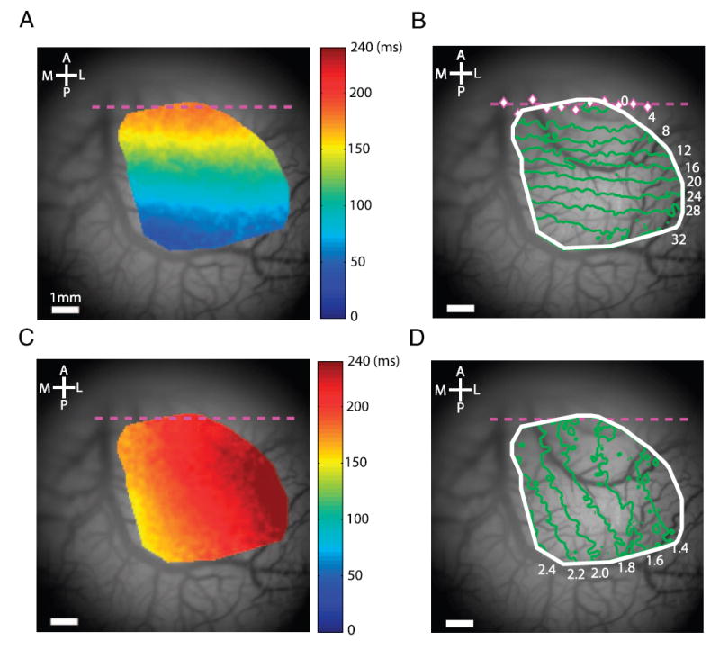
Retinotopic map. A: time-to-peak map generated by a radial wedge moving in the counterclockwise direction. Gray background of cortical vasculature, cortical regions for which latency could not be reliably estimated (see METHODS). B: polar angle component of the retinotopic map measured relative to the lower vertical meridian. Magenta diamonds indicate the locations of phase reversals in narrow vertical strips (0.552 mm wide, 0.552 mm apart) extending through the V1/V2 border region. Dashed magenta line is the best-fit linear regression line through these phase reversal points and represents the approximate location of the V1/V2 border used in all other figures. C: time-to-peak map generated by a ring segment moving inward. D: eccentricity component of the retinotopic map.
FIG. 7.
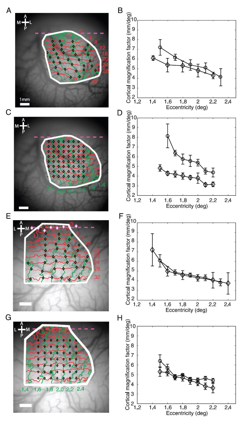
Cortical magnification. A: sampled locations in the retinotopic map for computing cortical magnification factors along isopolar contours and along isoeccentricity contours (black diamonds). B: cortical magnification factors along isopolar contours (circle) and along isoeccentricity contours (diamond) as a function of eccentricity. C: sampled locations on the retinotopic map for computing cortical magnification factors parallel and normal to the V1/V2 border. D: cortical magnification factors parallel (circle) and normal (diamonds) to the V1/V2 border as a function of eccentricity. E: retinotopic map obtained from the left hemisphere of a second monkey. Magenta diamonds indicate the locations of phase reversals in narrow vertical strips (0.552 mm wide, 0.552 mm apart) extending through the V1/V2 border region. Dashed magenta line is the best-fit linear regression line through these phase reversal points and represents the approximate location of the V1/V2 border. Black diamonds indicate the sampled locations in the retinotopic map for computing cortical magnification factors along isopolar contours and along isoeccentricity contours. F: cortical magnification factors along isopolar contours (circle) and along isoeccentricity contours (diamond) as a function of eccentricity in the second monkey. G: sampled locations on the retinotopic map of the second monkey for computing cortical magnification factors parallel and normal to the V1/V2 border. H: cortical magnification factors parallel (circle) and normal (diamonds) to the V1/V2 border as a function of eccentricity in the second monkey.
We next examined the reproducibility of these maps.
Reproducibility of retinotopic maps
The maps generated by this protocol were highly reproducible within the same experiment and across experiments. Figure 5, A and B shows the polar and eccentricity maps of V1 obtained separately from all odd trials (red traces) and all even trials (green traces) in one experiment. The average distances between the results from the odd and even trials were 0.046 mm for the polar map and 0.104 mm for the eccentricity map. These small differences corresponded to an average difference of 0.011° of visual angle in the polar map and 0.019° of visual angle in the eccentricity map.
We next compared the retinotopic map obtained from the experiment shown in Fig. 5, A and B with the polar and eccentricity maps obtained from a second experiment in the same hemisphere. In this experiment the camera was located at a slightly different position, allowing us to map retinotopy in different but partially overlapping regions of V1. To compare maps obtained in different experiments, we used an alignment algorithm to find the affine transformation that minimized the difference between the images of the vasculature from the two experiments (see METHODS). This affine transformation was then applied to the retinotopic maps from the two experiments and the two maps were overlaid in the region in which they overlapped (Fig. 5, C and D).
There was good agreement between the maps in the overlapping regions. The average distances between the retinotopic coordinates were 0.13 mm for the polar map and 0.24 mm for the eccentricity map. These small differences corresponded to an average difference of 0.028° of visual angle for the polar map and 0.045° for the eccentricity map. The fact that these differences were higher than those obtained from nonoverlapping trials in the same experiments suggests that some of the differences could be explained by errors in the alignment procedure. The correspondence between retinotopic maps acquired on different days was particularly encouraging, given that these experiments were conducted in behaving monkeys with imperfect fixation. Our results demonstrate that despite the variability introduced by small fixational eye movements, high-precision and highly reproducible retinotopic maps can be obtained. A detailed analysis of the effects of fixational eye movements is given below.
Possible effect of eye movement
During the imaging period the eyes were quite stable. The average SD of the eye position within individual trials was 0.496°. The variation in eye position across trials was somewhat higher (SD of the average eye position across trials, 0.82°). This additional variability was attributed to slow changes in the initial eye position across trials. We suspected that these slow changes were the result of a drift in the signal acquired from the eye tracker.
To examine this possibility, we analyzed the eye position signal in a separate experimental session in which one of the two monkeys was required to make saccadic eye movements to a small, high-contrast, visual target. For each trial, we computed the eye position in the 400 ms before saccade onset and in the 100 ms after the saccade. We then computed the horizontal and vertical components of the deviation from the mean position before and after each saccade. If slow drifts in the eye tracker signal contributed to the variability in the initial eye position across trials, we would expect the deviations in the eye position before the saccade and after the saccade to be highly correlated. Consistent with this possibility, we found that the average correlation coefficient over eight experiments was 0.64 for the horizontal offset and 0.61 for the vertical offset (total of 222 saccades). These results indicate that a large fraction of the observed variability in the initial eye position arose from slow drifts in the eye tracker signal.
We also examined possible differences in fixation between the stimulus conditions because such variations could distort the estimated retinotopic maps. We computed the average eye position in all trials of a given stimulus condition. Differences in the average eye position between the blank trials and the moving stimuli and single-frame conditions were small (average difference <0.1°) and not statistically significant (P > 0.05, t-test), indicating that our maps are not likely to be distorted by differences in fixations between stimulus conditions.
Consistency with responses to small localized stimuli
To confirm our analysis methods, we compared the retinotopic maps obtained from the moving stimuli with responses produced by single stationary wedges or ring segments (see METHODS). Figure 6A shows the locations with the shortest time-to-peak in response to single wedges centered at 237.5 angular deg (blue symbols), 252.5° (green symbols), and 267.5° (red symbols). The three colored curves indicate the corresponding retinotopic coordinates from the retinotopic map in Fig. 4B. The two measurements were in close agreement (average distance between predicted and observed, 0.17 mm).
Similarly, Fig. 6B shows the locations with the shortest time-to-peak in response to single ring segments centered at eccentricities of 1.92° (red symbols) and 2.16° (green symbols). The two colored curves indicate the corresponding retinotopic coordinates from the retinotopic map in Fig. 4D. As with the polar map, the two measurements were in close agreement (mean distance between predicted and observed, 0.16 mm).
Our method for computing the retinotopic map relies on the assumption that the neural latency of the response (i.e., the time-to-peak of the response to a stimulus that directly activates the receptive field of the neurons at a given cortical location) is constant across the mapped area. To test this assumption, we computed the neural latency (the shortest time-to-peak relative to stimulus onset) for each of the five stationary stimuli (two rings and three wedges), at each of five narrow ROIs. For measuring the latency in response to the single wedges, we measured the shortest time-to-peak in five thin vertical strips in Fig. 6A (gray rectangles, 0.276 mm wide, 0.552 mm apart). For measuring the latency in response to the single ring segments, we measured the shortest time-to-peak in five thin horizontal strips in Fig. 6B (gray rectangles, 0.276 mm wide, 0.552 mm apart). The neural latency was very similar for the five stimuli at all five locations (mean latency = 109.2 ms; SD = 5.8 ms), indicating that the latency of the neural response was fairly constant across V1.
Estimation of cortical magnification factors
We used the detailed retinotopic maps to measure the cortical magnification factor (CMF) within the mapped area. To calculate the linear CMF, we selected the intersections between isopolar contours and isoeccentricity contours (Fig. 7A, black symbols) and computed the average retinotopic coordinate in a region of 0.5 × 0.5 mm centered at each of the selected locations. CMF was then computed as the ratio of the cortical distance to the retinotopic distance between two neighboring locations. Figure 7B shows the CMF as a function of eccentricity along isopolar contours (circles) and along isoeccentricity contours (diamonds). As expected, CMF dropped as eccentricity increased (e.g., Tootell et al. 1988). CMF was almost the same along isoeccentricity curves and along isopolar curves showing weak anisotropy (the average ratio of CMF along isopolar contours to CMF along isoeccentricity contours was 1.14).
Stronger anisotropy was obtained when comparing CMF along the directions parallel to the V1/V2 border and normal to the V1/V2 border (Fig. 7, C and D). The average ratio of CMF parallel to and normal to the V1/V2 border was 1.51, more comparable to previous studies (e.g., Blasdel and Campbell 2001). CMF normal to the V1/V2 border was lower than that along isoeccentricity contours because isoeccentricity contours were curved laterally toward the foveal representation (Fig. 4D).
Results from the left hemisphere in the second monkey showed a similar pattern of CMF (Fig. 7, E–H). In this animal, however, there was no anisotropy along isopolar contours and isoeccentricity contours (average CMF ratio was 1.01), whereas the average ratio of CMF parallel to and normal to the V1/V2 border was 1.11. Such differences in the level of anisotropy could reflect individual variability in the organization of the retinotopic map (e.g., Van Essen et al. 1984).
Spatial precision of retinotopy in V1
To examine the spatial precision of the retinotopic maps, we performed a bootstrap procedure (see METHODS) that allowed us to estimate the 95% confidence interval for the retinotopic coordinate at each cortical location. Figure 8B shows the distribution of polar coordinates obtained from four sites in V1 that were 0.276 mm apart along a line normal to the V1/V2 border (colored symbols in Fig. 8A). Figure 8E shows the distribution of eccentricity coordinates obtained from four sites in V1 that were 0.276 mm apart along a line parallel to the V1/V2 border (colored symbols in Fig. 8D). There was very little overlap between the distributions of retinotopic coordinates at neighboring sites.
FIG. 8.
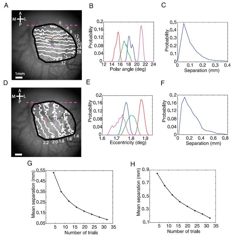
Precision of the retinotopic maps. A: map of polar angle and 4 selected locations (colored symbols) 0.276 mm apart for assessing spatial precision of retinotopy. B: bootstrapped distributions of the polar coordinates at the 4 color-coded locations in A. Distribution was obtained by a bootstrap procedure, sampling 28 trials with replacement from a total of 36 trials (see METHODS). C: distributions of the spatial separations at which the bootstrapped retinotopic coordinate distributions overlapped by <5% in response to the radial wedge moving in the counterclockwise direction. D–F: same as A–C, but for the eccentricity map. G: mean separation shown in C as a function of the number of trial repetitions. H: mean separation shown in F as a function of the number of trial repetitions.
Comparable precision was observed across all locations within the ROI (Fig. 8, C and F). The mean 95% confidence intervals were 0.11 mm for the polar map, which corresponds to 0.026° of visual angle (Fig. 8C), and 0.19 mm for the eccentricity map, which corresponds to 0.04° of visual angle (Fig. 8F). The mean 95% confidence intervals from the second monkey were 0.22 mm for the polar map and 0.33 mm for the eccentricity map with 15 repetitions per condition. A bootstrap analysis of the precision of the retinotopic map as a function of the number of repetitions per condition indicated that retinotopy with arbitrarily high precision could be obtained with a larger number of repeated measurements (Fig. 8, G and H).
DISCUSSION
By combining voltage-sensitive dye imaging with phase-encoding techniques, we were able to obtain high-precision retinotopic maps from V1 and V2 in two behaving monkeys. Maps that were obtained within <4 min of imaging had spatial precision <0.2 mm. We demonstrated that these maps are reliable and consistent across experiments. Furthermore, we showed that these maps can be used to predict the location of the response to small localized visual stimuli.
Our results show that the retinotopic map in macaque V1 is highly regular and precise. The retinotopic maps showed no evidence for reversals, fractures, or pronounced discontinuities. Our results are consistent with previous studies that demonstrated that the retinotopic map is precise down to the 100- to 200-micron level (Blasdel and Fitzpatrick 1984; Tootell et al. 1982, 1988). The precision of our measurements indicates that despite the relatively large point spread in V1 (e.g., Engel et al. 1997; Grinvald et al. 1994) and despite fixational eye movements, V1 population responses can support extremely precise localization of visual stimuli.
It may seem surprising that we can obtain retinotopic maps with a precision of 100–200 microns despite the monkeys’ fixational eye movements. Our analysis of the eye position signals suggests that the fixational eye movements were much smaller than the allowable fixation window. Furthermore, eye movements, as long as they are isotropic, only contribute to blurring the neural response, but do not limit the precision of the retinotopic maps. In fact, even in anesthetized animals, the point spread of the cortical response is an order of magnitude larger than the precision obtained in the current study (e.g., McLlwain 1986). What limits the precision of the retinotopic maps is the signal-to-noise ratio. Increase in the blurring due to eye movements can be compensated for by increasing the number of repetitions for each condition, as our bootstrap analysis demonstrated (Fig. 8).
In conclusion, we demonstrated that VSDI signals can reliably track the propagation of waves of neural population activity in the visual cortex. Combined with the methods developed here for detailed mapping of retinotopy in the cortex, these techniques could be used to study dynamic propagation of waves of activity in the visual cortex in response to other types of moving visual stimuli. The ability to precisely measure the propagation of cortical waves could be used to study the correlation between the spatiotemporal responses in V1 and behavior in a variety of perceptual tasks that involve dynamic visual stimuli. For example, these techniques could be used to measure cortical waves under conditions of binocular rivalry (Lee et al. 2005; Wilson et al. 2001).
Acknowledgments
We thank Y. Chen and W. Bosking for assistance with experiments and for discussions; T. Matsui, C. Michelson, and C. Palmer for discussions; and T. Cakic, C. Creeger, and M. Wu for technical support.
GRANTS This work was supported by National Eye Institute Grants EY-016454 to E. Seidemann and EY-016752 to D. J. Heeger and E. Seidemann and by a Sloan Foundation Fellowship to E. Seidemann.
References
- Adams DL, Horton JC. A precise retinotopic map of primate striate cortex generated from the representation of angioscotomas. J Neurosci. 2003;23:3771–3789. doi: 10.1523/JNEUROSCI.23-09-03771.2003. [DOI] [PMC free article] [PubMed] [Google Scholar]
- Allman JM, Kaas JH. The organization of the second visual area (V II) in the owl monkey: a second order transformation of the visual hemifield. Brain Res. 1974;76:247–265. doi: 10.1016/0006-8993(74)90458-2. [DOI] [PubMed] [Google Scholar]
- Arieli A, Grinvald A, Slovin H. Dural substitute for long-term imaging of cortical activity in behaving monkeys and its clinical implications. J Neurosci Methods. 2002;114:119–133. doi: 10.1016/s0165-0270(01)00507-6. [DOI] [PubMed] [Google Scholar]
- Beaton AE, Tukey JW. The fitting of power series, meaning polynomials, illustrated on band-spectroscopic data. Technometrics. 1974;16:147–185. [Google Scholar]
- Blasdel G, Campbell D. Functional retinotopy of monkey visual cortex. J Neurosci. 2001;21:8286–8301. doi: 10.1523/JNEUROSCI.21-20-08286.2001. [DOI] [PMC free article] [PubMed] [Google Scholar]
- Blasdel GG, Fitzpatrick D. Physiological organization of layer 4 in macaque striate cortex. J Neurosci. 1984;4:880–895. doi: 10.1523/JNEUROSCI.04-03-00880.1984. [DOI] [PMC free article] [PubMed] [Google Scholar]
- Bradley DC, Troyk PR, Berg JA, Bak M, Cogan S, Erickson R, Kufta C, Mascaro M, McCreery D, Schmidt EM, Towle VL, Xu H. Visuotopic mapping through a multichannel stimulating implant in primate V1. J Neurophysiol. 2005;93:1659–1670. doi: 10.1152/jn.01213.2003. [DOI] [PubMed] [Google Scholar]
- Brewer AA, Press WA, Logothetis NK, Wandell BA. Visual areas in macaque cortex measured using functional magnetic resonance imaging. J Neurosci. 2002;22:10416–10426. doi: 10.1523/JNEUROSCI.22-23-10416.2002. [DOI] [PMC free article] [PubMed] [Google Scholar]
- Chen Y, Geisler WS, Seidemann E. Optimal decoding of correlated neural population responses in the primate visual cortex. Nat Neurosci. 2006;9:1412–1420. doi: 10.1038/nn1792. [DOI] [PMC free article] [PubMed] [Google Scholar]
- Daniel PM, Witteridge D. The representation of the visual field on the cerebral cortex in monkeys. J Physiol. 1961;159:203–221. doi: 10.1113/jphysiol.1961.sp006803. [DOI] [PMC free article] [PubMed] [Google Scholar]
- DeYoe EA, Carman GJ, Bandettini P, Glickman S, Wieser J, Cox R, Miller D, Neitz J. Mapping striate and extrastriate visual areas in human cerebral cortex. Proc Natl Acad Sci USA. 1996;93:2382–2386. doi: 10.1073/pnas.93.6.2382. [DOI] [PMC free article] [PubMed] [Google Scholar]
- Dobelle WH, Turkel J, Henderson DC, Evans JR. Mapping the representation of the visual field by electrical stimulation of human visual cortex. Am J Ophthalmol. 1979;88:727–735. doi: 10.1016/0002-9394(79)90673-1. [DOI] [PubMed] [Google Scholar]
- Engel SA, Glover GH, Wandell BA. Retinotopic organization in human visual cortex and the spatial precision of functional MRI. Cereb Cortex. 1997;7:181–192. doi: 10.1093/cercor/7.2.181. [DOI] [PubMed] [Google Scholar]
- Engel SA, Rumelhart DE, Wandell BA, Lee AT, Glover GH, Chichilnisky EJ, Shadlen MN. fMRI of human visual-cortex. Nature. 1994;369:525–525. doi: 10.1038/369525a0. [DOI] [PubMed] [Google Scholar]
- Fize D, Vanduffel W, Nelissen K, Denys K, d’Hotel CC, Faugeras O, Orban GA. The retinotopic organization of primate dorsal V4 and surrounding areas: a functional magnetic resonance imaging study in awake monkeys. J Neurosci. 2003;23:7395–7406. doi: 10.1523/JNEUROSCI.23-19-07395.2003. [DOI] [PMC free article] [PubMed] [Google Scholar]
- Fox PT, Miezin FM, Allman JM, Vanessen DC, Raichle ME. Retinotopic organization of human visual-cortex mapped with positron-emission tomography. J Neurosci. 1987;7:913–922. doi: 10.1523/JNEUROSCI.07-03-00913.1987. [DOI] [PMC free article] [PubMed] [Google Scholar]
- Gattass R, Nascimento-Silva S, Soares JGM, Lima B, Jansen AK, Diogo ACM, Farias MF, Marcondes M, Botelho EP, Mariani OS, Azzi J, Fiorani M. Cortical visual areas in monkeys: location, topography, connections, columns, plasticity and cortical dynamics. Philos Trans R Soc Lond B Biol Sci. 2005;360:709–731. doi: 10.1098/rstb.2005.1629. [DOI] [PMC free article] [PubMed] [Google Scholar]
- Glickstein M, Whitteridge D. Tatsuji Inouye and the mapping of the visual field on the human cerebral cortex. Trends Neurosci. 1987;10:350–353. [Google Scholar]
- Grinvald A, Hildesheim R. VSDI: a new era in functional imaging of cortical dynamics. Nat Rev Neurosci. 2004;5:874–885. doi: 10.1038/nrn1536. [DOI] [PubMed] [Google Scholar]
- Grinvald A, Lieke EE, Frostig RD, Hildesheim R. Cortical point-spread function and long-range lateral interactions revealed by real-time optical imaging of macaque monkey primary visual-cortex. J Neurosci. 1994;14:2545–2568. doi: 10.1523/JNEUROSCI.14-05-02545.1994. [DOI] [PMC free article] [PubMed] [Google Scholar]
- Grinvald A, Shoham D, Shmuel A, Glaser DE, Vanzetta I, Shtoyerman E, Slovin H, Wijnbergen C, Hildesheim R, Sterkin A, Arieli A. In-vivo optical imaging of cortical architecture and dynamics. In: Windhorst U, Johansson H, editors. Modern Techniques in Neuroscience Research. New York: Springer; 1999. pp. 893–969. [Google Scholar]
- Hampel FR, Ronchetti EM, Rousseeuw PJ, Stahel WA. Robust Statistics: The Approach Based on Influence Functions. New York: Wiley; 1986. [Google Scholar]
- Holland PW, Welsch RE. Robust regression using iteratively reweighted least-squares. Commun Stat Theory Methods A. 1977;6:813–827. [Google Scholar]
- Holmes G. The organization of the visual cortex in man. Proc R Soc Lond B Biol Sci. 1945;132:348–361. [Google Scholar]
- Horton JC, Hoyt WF. The representation of the visual field in human striate cortex a revision of the classic Holmes map. Arch Ophthalmol. 1991;109:816–824. doi: 10.1001/archopht.1991.01080060080030. [DOI] [PubMed] [Google Scholar]
- Hubel DH, Weisel TN. Shape and arrangement of columns in cat’s striate cortex. J Physiol. 1963;165:559–568. doi: 10.1113/jphysiol.1963.sp007079. [DOI] [PMC free article] [PubMed] [Google Scholar]
- Hubel DH, Wiesel TN. Uniformity of monkey striate cortex: a parallel relationship between field size, scatter and magnification factor. J Comp Neurol. 1974;158:295–306. doi: 10.1002/cne.901580305. [DOI] [PubMed] [Google Scholar]
- Hubel DH, Weisel TN. Ferrier lecture. Functional architecture of macaque monkey visual cortex. Proc R Soc Lond B Biol Sci. 1977;198:1–59. doi: 10.1098/rspb.1977.0085. [DOI] [PubMed] [Google Scholar]
- Jancke D, Chavane F, Naaman S, Grinvald A. Imaging cortical correlates of illusion in early visual cortex. Nature. 2004;428:423–426. doi: 10.1038/nature02396. [DOI] [PubMed] [Google Scholar]
- Kalatsky VA, Stryker MP. New paradigm for optical imaging: temporally encoded maps of intrinsic signal. Neuron. 2003;38:529–545. doi: 10.1016/s0896-6273(03)00286-1. [DOI] [PubMed] [Google Scholar]
- Knudsen EI, Lac S, Esterly SD. Computational maps in the brain. Annu Rev Neurosci. 1987;10:41–65. doi: 10.1146/annurev.ne.10.030187.000353. [DOI] [PubMed] [Google Scholar]
- Larsson J, Heeger DJ. Two retinotopic visual areas in human lateral occipital cortex. J Neurosci. 2006;26:13128–13142. doi: 10.1523/JNEUROSCI.1657-06.2006. [DOI] [PMC free article] [PubMed] [Google Scholar]
- Lee SH, Blake R, Heeger DJ. Traveling waves of activity in primary visual cortex during binocular rivalry. Nat Neurosci. 2005;8:22–23. doi: 10.1038/nn1365. [DOI] [PMC free article] [PubMed] [Google Scholar]
- McLlwain JT. Point images in the visual system: new interest in an old idea. Trends Neurosci. 1986;9:354–358. [Google Scholar]
- Mountcastle VB. Modality and topographic properties of single neurons of cat’s somatic sensory cortex. J Neurophysiol. 1957;20:408–434. doi: 10.1152/jn.1957.20.4.408. [DOI] [PubMed] [Google Scholar]
- Nestares O, Heeger DJ. Robust multiresolution alignment of MRI brain volumes. Magn Reson Med. 2000;43:705–715. doi: 10.1002/(sici)1522-2594(200005)43:5<705::aid-mrm13>3.0.co;2-r. [DOI] [PubMed] [Google Scholar]
- Polimeni JR, Balasubramanian M, Schwartz EL. Multi-area visuotopic map complexes in macaque striate and extra-striate cortex. Vision Res. 2006;46:3336–3359. doi: 10.1016/j.visres.2006.03.006. [DOI] [PMC free article] [PubMed] [Google Scholar]
- Seidemann E, Arieli A, Grinvald A, Slovin H. Dynamics of depolarization and hyperpolarization in the frontal cortex and saccade goal. Science. 2002;295:862–865. doi: 10.1126/science.1066641. [DOI] [PubMed] [Google Scholar]
- Sereno MI, Dale AM, Reppas JB, Kwong KK, Belliveau JW, Brady TJ, Rosen BR, Tootell RBH. Borders of multiple visual areas in humans revealed by functional magnetic-resonance-imaging. Science. 1995;268:889–893. doi: 10.1126/science.7754376. [DOI] [PubMed] [Google Scholar]
- Shoham D, Glaser DE, Arieli A, Kenet T, Wijnbergen C, Toledo Y, Hildesheim R, Grinvald A. Imaging cortical dynamics at high spatial and temporal resolution with novel blue voltage-sensitive dyes. Neuron. 1999;24:791–802. doi: 10.1016/s0896-6273(00)81027-2. [DOI] [PubMed] [Google Scholar]
- Slovin H, Arieli A, Hildesheim R, Grinvald A. Long-term voltage-sensitive dye imaging reveals cortical dynamics in behaving monkeys. J Neurophysiol. 2002;88:3421–3438. doi: 10.1152/jn.00194.2002. [DOI] [PubMed] [Google Scholar]
- Talbot SA, Marshall WH. Physiological studies on neural mechanisms of visual localization and discrimination. Am J Ophthalmol. 1941;24:1255–1264. [Google Scholar]
- Tootell RBH, Silverman MS, Switkes E, Devalois RL. Deoxyglucose analysis of retinotopic organization in primate striate cortex. Science. 1982;218:902–904. doi: 10.1126/science.7134981. [DOI] [PubMed] [Google Scholar]
- Tootell RBH, Switkes E, Silverman MS, Hamilton SL. Functional-anatomy of macaque striate cortex. 2. Retinotopic organization. J Neurosci. 1988;8:1531–1568. doi: 10.1523/JNEUROSCI.08-05-01531.1988. [DOI] [PMC free article] [PubMed] [Google Scholar]
- Van Essen DC, Newsome WT, Maunsell JHR. The visual field representation in striate cortex of the macaque monkey: asymmetries, anisotropies, and individual variability. Vision Res. 1984;24:429–448. doi: 10.1016/0042-6989(84)90041-5. [DOI] [PubMed] [Google Scholar]
- Van Essen DC, Zeki SM. The topographic organization of rhesus monkey prestriate cortex. J Physiol. 1978;277:193–226. doi: 10.1113/jphysiol.1978.sp012269. [DOI] [PMC free article] [PubMed] [Google Scholar]
- Wandell BA, Brewer AA, Dougherty RF. Visual field map clusters in human cortex. Philos Trans R Soc Lond B Biol Sci. 2005;360:693–707. doi: 10.1098/rstb.2005.1628. [DOI] [PMC free article] [PubMed] [Google Scholar]
- Wilson HR, Blake R, Lee SH. Dynamics of travelling waves in visual perception. Nature. 2001;412:907–910. doi: 10.1038/35091066. [DOI] [PubMed] [Google Scholar]
- Woolsey CN. The Biology of Mental Health and Disease. New York: Hoeber; 1952. Patterns of localization in sensory and motor areas of the cerebral cortex; pp. 193–206. [Google Scholar]