Properties of Single Voltage-gated Proton Channels in Human Eosinophils Estimated by Noise Analysis and by Direct Measurement

Abstract

Voltage-gated proton channels were studied under voltage clamp in excised, inside-out patches of human eosinophils, at various pH_i with pH_o 7.5 or 6.5 pipette solutions. H⁺ current fluctuations were observed consistently when the membrane was depolarized to voltages that activated H⁺ current. At pH_i ≤ 5.5 the variance increased nonmonotonically with depolarization to a maximum near the midpoint of the H⁺ conductance-voltage relationship, g _H-V, and then decreased, supporting the idea that the noise is generated by H⁺ channel gating. Power spectral analysis indicated Lorentzian and 1/f components, both related to H⁺ currents. Unitary H⁺ current amplitude was estimated from stationary or quasi-stationary variance, . We analyze data obtained at various voltages on a linearized plot that provides estimates of both unitary conductance and the number of channels in the patch, without requiring knowledge of open probability. The unitary conductance averaged 38 fS at pH_i 6.5, and increased nearly fourfold to 140 fS at pH_i 5.5, but was independent of pH_o. In contrast, the macroscopic g _H was only 1.8-fold larger at pH_i 5.5 than at pH_i 6.5. The maximum H⁺ channel open probability during large depolarizations was 0.75 at pH_i 6.5 and 0.95 at pH_i 5.5. Because the unitary conductance increases at lower pH_i more than the macroscopic g _H, the number of functional channels must decrease. Single H⁺ channel currents were too small to record directly at physiological pH, but at pH_i ≤ 5.5 near V _threshold (the voltage at which g _H turns on), single channel–like current events were observed with amplitudes 7–16 fA.

INTRODUCTION

Voltage-gated proton channels differ in several respects from other voltage-gated ion channels. Indeed, it is still debated whether they are ion channels or carriers. Like ion channels, H⁺ channels conduct protons passively down their electrochemical gradient, and independently of other ionic species. They probably do not meet a narrow definition of an ion channel as a water-filled pore through which ions diffuse, because the mechanism of permeation is believed to be radically different. Proton channels appear to conduct by a Grotthuss-like mechanism in which protons hop across a hydrogen-bonded chain spanning the membrane (Nagle and Morowitz, 1978; DeCoursey, 2003). Several distinctive properties of voltage-gated proton channels are likely a consequence of this unique conduction mechanism. H⁺ channels are extremely selective for H⁺ (P _H/P _cation > 10⁶) (DeCoursey and Cherny, 1994). H⁺ conduction has much greater temperature dependence (Byerly and Suen, 1989; Kuno et al., 1997; DeCoursey and Cherny, 1998) and stronger deuterium isotope effects (DeCoursey and Cherny, 1997) than the vast majority of ion channels. Nevertheless, H⁺ permeates passively down its electrochemical gradient, and H⁺ channels exhibit time- and voltage-dependent gating, and thus resemble ion channels more than other transporters. If proton channels are genuine voltage-gated ion channels, their gating ought to generate current fluctuations that could be used to estimate the single channel conductance. The H⁺ current fluctuations described here provide strong evidence of gating, a defining property of ion channels, and thus support the designation of voltage-gated proton channels as genuine ion channels

Three groups have attempted to detect H⁺ current fluctuations previously (Byerly and Suen, 1989; Bernheim et al., 1993; DeCoursey and Cherny, 1993). In the best case, the signal-to-noise ratio (S/N = the ratio of H⁺ current variance to the “background” variance when H⁺ channels are closed or blocked) was very poor, 0.5 (DeCoursey and Cherny, 1993). Byerly and Suen (1989) established an upper bound at <50 fS at pH_i 5.9. No excess fluctuations were seen (S/N = 0), but the data had to be filtered at 1 kHz because of the rapid gating kinetics in snail neurons. Bernheim et al. (1993) filtered at 5 kHz, and from a 6% reduction of variance in the presence of Cd²⁺ (S/N = 0.06), they estimated the conductance to be 90 fS at pH_i 5.5 (Bernheim et al., 1993). DeCoursey and Cherny (1993) improved S/N to 0.5 and estimated the unitary conductance at pH_i 6.0 in human neutrophils to be ∼10 fS. All of these estimates were compromised by poor S/N and should be considered very rough. Here we report noise measurements in which S/N was routinely >100 and sometimes >1,000. In whole-cell studies, stationary H⁺ current fluctuations can only be recorded just above V _threshold because prolonged H⁺ currents deplete intracellular buffer and change pH_i (Thomas and Meech, 1982; DeCoursey, 1991). To avoid this problem, we studied noise in excised inside-out patches. An additional benefit is that this approach enables varying pH_i in the same experiment.

MATERIALS AND METHODS

Eosinophil Isolation

Venous blood was drawn from healthy adult volunteers under informed consent according to procedures approved by our Institutional Review Board and in accordance with federal regulations. Neutrophils were isolated by density gradient centrifugation as described previously (DeCoursey et al., 2001) with one modification. In the two cycles of hypotonic lysis performed for removal of the red blood cells, isotonicity was restored by the addition of 2× concentrated Hank's balanced salt solution (HBSS)* (without Ca²⁺ or Mg²⁺) containing 5 mM HEPES, pH 7.4. Eosinophils were isolated from the neutrophil preparation by negative selection using anti-CD16 immunomagnetic beads as described by the manufacturer (Miltenyi Biotec, Inc.). The eosinophils were suspended in HEPES (10 mM)-buffered HBSS (with Ca²⁺ and Mg²⁺), pH 7.4, containing 1 mg/ml human serum albumin (HEPES-HBSS-HSA buffer). Eosinophil purity was routinely >98% as determined by counting Wright-stained cytospin preparations.

Solutions

External and internal solutions contained 100 or 200 mM buffer supplemented with tetramethylammonium methanesulfonate (TMAMeSO₃) to bring the osmolality to ∼300 mosmol kg⁻¹. Solutions contained 2 mM MgCl₂ and 1 mM EGTA. Solutions were titrated to the desired pH with tetramethylammonium hydroxide (TMAOH) or methanesulfonic acid (for solutions using BisTris as a buffer). A stock solution of TMAMeSO₃ was made by neutralizing TMAOH with methanesulfonic acid. The following buffers were used near their pK _a (at 20°C) for measurements at the following pH: pH 4.1, phosphate (phosphoric acid neutralized with TMAOH); pH 5.0, Homopipes (homopiperazine-N,N'-bis-2-(ethanesulfonic acid), pK _a 4.61); pH 5.5–6.0 Mes (pK _a 6.15); pH 6.5 Bis-Tris (bis[2-hydroxyethyl]imino-tris[hydroxymethyl]methane, pK _a 6.50); pH 7.5 HEPES (pK _a 7.55). Buffers were purchased from Sigma-Aldrich, except for Homopipes (Research Organics). In about half the experiments, solutions with 200 mM HEPES for pH 7.5 or 200 mM Mes for pH 5.5 and 6.5 were used. These solutions contained 2 mM MgCl₂ and 2 mM EGTA and were titrated to the desired pH with n-methyl-D-glucamine or with TMAOH.

TΩ seals.

The seal resistance in this study was typically in the TΩ (10¹² Ω) range. Our solutions were designed to minimize extraneous conductances by use of impermeant ions and to maximize control of pH by use of high buffer concentrations. The ionic strength was lower than more conventional solutions, especially for the 200 mM buffer solutions. Consequently, the conductivity of these solutions measured at 25°C with a Fisher Digital Conductivity Meter (Fisher Scientific) was low: 7.2–9.8 mS/cm for the 100 mM buffer solutions and 2.7–7.3 mS/cm for the 200 mM buffer solutions, compared, for example, with 15.9 mS/cm for Ringer's and 22.4 mS/cm for isotonic K⁺ Ringer's solutions. Both the low conductivity and the paucity of permeant ions may have contributed to the high seal resistances obtained. The patch resistance at voltages negative to the threshold for activating H⁺ currents averaged 1.33 ± 0.18 TΩ (mean ± SEM, n = 20) in patches studied with 100//100 mM buffer (out//in). With the 200//200 mM buffer solutions, the patch resistance was no higher, 1.32 ± 0.15 TΩ (n = 21). There was no significant difference between resistances measured in any two combinations of solutions. High resistance patches are not cell specific; a 0.9 TΩ resistance was obtained in an alveolar epithelial cell patch studied with similar solutions (Fig. 15 of DeCoursey, 2003). Resistances up to 4 TΩ were reported by Benndorf (1994), using hypertonic solutions (conductivity 36.6 mS/cm) and tiny pipette openings of only 0.2 μm (∼70 MΩ pipette resistance even with the highly conductive solution). Our pipettes had “normal” geometry and typically a 5–15 MΩ tip resistance.

Electrophysiology

All measurements were made using the inside-out patch configuration. Inside-out patches were formed by obtaining a tight seal and then lifting the pipette into the air briefly. Micropipettes were pulled using a Flaming Brown automatic pipette puller (Sutter Instruments Co.) from 7052 glass (Garner Glass Co.), coated with Sylgard 184 (Dow Corning Corp.), and heat polished. Electrical contact with the pipette solution was achieved by a thin sintered Ag-AgCl pellet (In Vivo Metric Systems) attached to a Teflon-encased silver wire. A reference electrode made from a Ag-AgCl pellet was connected to the bath through an agar bridge made with Ringer's solution. The current signal from the patch clamp (List Electronic) was passed through a secondary 8-pole lowpass Bessel filter (Frequency Devices model 902LPF) that was used to filter and amplify the signal by 20 dB, generally with a −3 dB cutoff frequency of 10–20 Hz. The minimum increment of digitization with a gain of 2,000 or 5,000 was ∼2.2 fA or ∼0.9 fA, respectively. The current was recorded simultaneously on both an Indec Laboratory Data Acquisition and Display System (Indec Corporation) and on a PC-based system with our own software written for the L780 ADC board (Measurement Computing Corp.). Seals were formed with Ringer's solution (in mM: 160 NaCl, 4.5 KCl, 2 CaCl₂, 1 MgCl₂, 5 HEPES, pH 7.4) in the bath, and the zero current potential established after the pipette was in contact with the cell. Then the bath was exchanged with one of the solutions described above. Bath temperature was controlled by Peltier devices, and monitored by a resistance temperature detector element (Omega Scientific) in the bath. The experiments were done at 21°C.

To calculate conductance, it is necessary to estimate the reversal potential, V _rev. This was done by conventional tail current analysis in patches in which the currents were large enough that tail currents could be resolved. In other patches, V _rev was estimated from the voltage at which H⁺ current first became activated, V _threshold, according to the empirical relationship between V _rev and V _threshold reported in Fig. 11 of DeCoursey and Cherny (1997), which appears to apply to voltage-gated proton channels in all cells (Fig. 19 in DeCoursey, 2003).

Figure 11.

The Lorentzian variance (▴) and the band-limited 1/f (○) and white noise (▾) variances were determined from fitted power spectra (Fig. 10) and are plotted here against membrane voltage (V). The white noise and 1/f variances were calculated over the interval [f ₀, f _N], where f ₀ is the lowest frequency in the spectrum and f _N is the Nyquist frequency. On average, the band-limited Lorentzian variance (open symbols in Fig. 4) was ∼10% less than the total Lorentzian variance (which is plotted here). The dashed lines without symbols show the calculated sum of the Johnson- and shot-noise variances (see Fig. 10) over the interval [f ₀, f _N]. (A) pH_o = 7.5, pH_i = 5.5, V _threshold = −55 mV; (B) pH_o = 7.5, pH_i = 6.5, V _threshold < −30 mV. Same two patches as in Fig. 10. In A, 1/f noise was not detectable between −10 and 20 mV; presumably it was masked by the Lorentzian. On the other hand, only 1/f noise was detected at 40 mV; apparently Lorentzian noise had fallen to undetectable levels, suggesting a P _max value close to unity. In B, no peak is observed in the Lorentzian variance, suggesting P _max ≤ 0.8 (see text and Fig. 5).

Conventions. We refer to pH in the format pH_o//pH_i. In the inside-out patch configuration the solution in the pipette sets pH_o, defined as the pH of the solution bathing the original extracellular surface of the membrane, and the bath solution sets pH_i. Currents and voltages are presented in the normal sense, that is, upward currents represent current flowing outward through the membrane from the original intracellular surface, and potentials are expressed by defining as 0 mV the original bath solution. Data are presented without correction for leak current or liquid junction potentials.

Evaluation of Adequacy of Noise Sample Duration

If a current sample is too short in relation to the time constants of the kinetic processes responsible for generating the noise, then σ ² will be underestimated (Diggle, 1990). To estimate the extent to which σ ² is underestimated by using finite records we pooled successive single records to form longer composite records and then determined σ ² as a function of sample length for each composite record. Plots like those in Fig. 1 were fitted with the following empirical function:

or one of its reduced forms (single exponential, exponential plus straight line). Models were chosen by considering the probability of Student's t values for the parameter estimates, followed by visual inspection. The “true” value of σ ² (σ ² _∞) was then estimated by extrapolating the saturating (exponential) components as t → ∞. 61 composite records were obtained from seven different patches, and included various suprathreshold voltages at pH_o 7.5 and 6.5, and pH_i 5.0, 5.5, and 6.5. Single record lengths ranged from 12 to 50 s, but were mostly 12–20 s. Composite-record lengths ranged from 16 to 166 s (two 16 s single records are included).

Figure 1.

Effect of sample length (Δt) on estimates of the current variance (σ ²). (A) pH_o//pH_i 7.5//5.0, V = −30 mV; the curve is a least-squares fit of with A ₀ = 4.0 × 10⁻²⁷ A², A ₁ = 1.5 × 10⁻²⁶ A², A ₂ = 2.0 × 10⁻²⁷ A², τ ₁ = 1.1 s and τ ₂ = 9.3 s. (B) pH_o//pH_i 7.5//6.5, V = 10 mV; the curve is a least-squares fit of , with A ₀ = 7.2 × 10⁻²⁹ A², A ₁ = 7.6 × 10⁻²⁸ A², τ ₁ = 1.3 s and B = 1.3 × 10⁻³⁰ A² s⁻¹. See text for details.

Values of σ ²(single-record)/σ ² _∞ ranged from 0.72 to 1.34, with a median of 0.99. [Some values of σ ²(single-record)/σ ² _∞ exceed unity because of scatter and/or the presence of a linear component.] Hence, errors in σ ² resulting from the use of finite (single) records appear to be negligible. Furthermore, there was no evidence that this error varied with pH_i. The presence of a linear (nonsaturating) component in 20 composite records (e.g., Fig. 1 B) apparently reflects the presence of 1/f noise, since the slope of the linear component was positively correlated with the band-limited variance of 1/f noise (unpublished data).

Spectral Analysis

For the determination of power spectra, the mean current was first subtracted from the current records. Records in which the current increased were fitted by linear or rising exponential functions, which were subtracted to eliminate spurious trends. The resulting residual time series were then analyzed by one of two methods. For pH regimes 7.5//5.0 and 7.5//5.5 (relatively fast kinetics), power spectra were obtained with program “spctrm” in Press et al. (1992). This program divides the data into at least two segments, estimates the spectral density for each segment using an FFT (fast Fourier transform), and then takes the average. Where several successive records at a given voltage were available, each record was treated as a segment. This gives the lowest frequency obtainable, because equally spaced data are required. Hence, the length of a segment (the reciprocal of which determines the lowest frequency) cannot exceed the length of a record when there are gaps between records. With this lower frequency limit, Lorentzian plateaus often were not detected for pH regimes 7.5//6.5 and 6.5//6.5, presumably because the slower gating kinetics shifted the Lorentzian component to lower frequencies than those resolved. Accordingly, a second method for determining power spectra was used for these data that allowed successive records (including gaps) to be treated as a single record, thus reducing the lower frequency limit of the spectrum. Gaps between records pose no problem for the estimation of the autocovariance function, which was calculated according to Eq. 2.5.5 in Diggle (1990). The one-sided spectral density was then obtained as the Fourier cosine transform of the autocovariance (Blackman-Tukey method) as described by Otnes and Enochson (1978). The reliability of both methods for estimating power spectra was checked with simulated data for a two-state kinetic scheme.

To correct for filtering, spectra were divided by the square modulus of the transfer function for an eight-pole low-pass Bessel filter using equation 3.11 and coefficients in Tietze and Schenk (1978). This had a negligible effect on most of the spectrum, but it did allow curve-fitting up to about the cutoff frequency of the filter (typically 20 Hz); data above this frequency were discarded. The data were then binned in log₁₀(f) intervals of 0.2 (where f is the frequency in Hz) before fitting with various functions by nonlinear least squares. The most general function employed treats the one-sided spectral density G(f) as the sum of Lorentzian, 1/f and white components:

where is the current variance attributed to open/closed transitions of the channels, τ _L is the “Lorentzian” time constant defined as (2πf _c)⁻¹, where f _c is the corner (half-power) frequency, and m, A, and B are constants. In practice, estimates of m were in the range 0.7 to 1.4; noise of this type is generally described as 1/f (Neumcke, 1978; DeFelice, 1981). Various reduced models were then fitted by removing one or more of these adjustable parameters. Initial selection of a minimum-parameter model was made using F-tests as described by Gallant (1975) and Walpole and Myers (1978). The fits were then checked visually and t-value probabilities for parameter estimates were inspected; in a few cases, the initial choice of minimum-parameter model was overridden.

Online Supplemental Material

The online supplemental material (available at http://www.jgp.org/cgi/content/full/jgp.200308813/DC1) evaluates quantitatively the possibility that pH changes due to H⁺ current might occur under the conditions of these experiments, and we estimate the errors introduced. Analysis of simulated y-g _H plots (e.g., Fig. 6) suggests that the errors in γ _H and N due to proton depletion/accumulation are relatively small and essentially independent of pH_i and pH_o. For typical values, γ _H was overestimated by 1–4% while N was underestimated by 2–10%. We also estimate that local pH changes due to current flow will be established within 0.1–1.2 s.

Figure 6.

Simultaneous estimation of γ_H and N at three pH_i in the same patch and with the same symbol meanings as in Figs. 2–4. The data set includes many records and different voltages. The lines are least-squares fits of Eq. 2, in which the Y-intercept is γ_H and the slope is −1/N, providing the following estimates: γ_H 36 fS, 181 fS, and 375 fS, and N 1210, 290, and 170 for pH_i 6.5, 5.5, and 5.0, respectively. ES-2596.

RESULTS

H⁺ Channel Gating Generates Current Fluctuations

The currents in excised patches were distinctly noisier when the H⁺ conductance was activated. Fig. 2 illustrates currents recorded during pulses or prolonged depolarizations in the same inside-out patch of membrane from a human eosinophil, at three different pH_i (the bath solution faces the intracellular side of the membrane). The threshold voltage, V _threshold, at which H⁺ current is first activated is exquisitely sensitive to pH, becoming more negative at lower pH_i, as in all other cells with voltage-gated proton channels (Byerly et al., 1984; DeCoursey, 2003). The patch currents exhibit little noise at subthreshold voltages, but become markedly noisier when small outward H⁺ current is activated just above V _threshold.

Figure 2.

Current fluctuations occur at voltages that activate voltage-gated proton current. Families of currents at pH_o 7.5 and three pH_i in the same membrane patch are illustrated at the same time and current calibrations. Raw currents are shown at 20-mV intervals, as indicated, with no leak correction. The holding potential was −100 mV at pH_i 5.0 and −80 mV for pH_i 5.5. The currents shown were obtained at 11–46 min for pH_i 6.5, 81 min for pH_i 5.5, and 83 min for pH_i 5.0, respectively, after patch excision. Filter was 20 Hz for all. ES-2596.

In Fig. 3 , chord conductance-voltage (g _H-V) relationships from the experiment in Fig. 2 are plotted. The curves show that the quasisteady-state g _H-V relationship is well described by a Boltzmann function. The slope factors are 5–8 mV, somewhat steeper than most estimates of 7–14 mV in whole-cell studies using shorter pulses (DeCoursey and Cherny, 1994; Cherny et al., 2001). The average slope factors were 8.16 ± 0.52 mV (mean ± SEM, n = 13) at pH 7.5//5.5 and 6.99 ± 0.48 mV (n = 16) at pH 7.5//6.5 (P > 0.1). The present values are probably more reliable for two reasons. First, they are more nearly steady-state, because they were measured after long times at each voltage. Second, H⁺ currents in excised patches are less distorted than in whole-cell configuration by pH changes that occur during current flow, due to depletion of protonated buffer (see online supplemental material, available at http://www.jgp.org/cgi/content/full/jgp.200308813/DC1).

Figure 3.

Steady-state g _H-V relationships for the patch illustrated in Fig. 2. Chord conductance, g _H, was calculated assuming V _rev of −40, −80, and −100 mV, at pH_i 6.5 (•), 5.5 (▪), and 5.0 (▴), respectively. Curves show best-fitting (by nonlinear least squares) Boltzmann functions: g _H = g _H,max {1 + exp[−(V − V _1/2)/k]}⁻¹ with midpoints (V _1/2) of −10.4, −26.9, and −43.0 mV, slope factors (k) of 5.2, 7.8, and 8.1 mV, and g _H,max of 32.6, 48.7, and 62.2 pS at pH_i 6.5, 5.5, and 5.0, respectively. ES-2596.

As evident in Fig. 3, lowering pH_i shifts the g _H-V relationship toward more negative voltages and increases g _H,max. The average shift in V _threshold between pH_i 6.5 and 5.5 was −36 ± 5 mV (mean ± SD, n = 9) and the average shift in the midpoint of the g _H-V relationship was −31 ± 9 mV (n = 8). Thus, in most patches, there was a larger shift in V _threshold than in the patch illustrated. Although this patch is not ideally representative in all respects, we use it in many figures in this paper because it was a rare patch in which we were able to record extensive data at three pH_i and it exhibits, at least qualitatively, all of the behaviors that characterize this system. The limiting g _H, g _H,max, consistently increased at lower pH_i. Rundown, which was often observed during long experiments (e.g., g _H,max might decrease 50%), compromises our comparison of g _H,max and of the number of channels in the patch, N, at different pH_i. However, measurements made before and after pH_i changes indicate that the macroscopic g _H,max has a relatively weak dependence on pH_i. On average, in nine patches in which sufficient data were recorded at both pH, g _H,max was 1.78 ± 0.10 (mean ± SE) times larger at pH_i 5.5 than 6.5 in each patch. This comparison was done with pH changes in both directions and the measurements were fairly close together in time to minimize effects of rundown.

Current fluctuations can be quantified by their variance, σ². Variance measured in the patch illustrated in Figs. 2 and 3 is plotted in Fig. 4 . Each data point represents a 12-s sample of current, collected during prolonged sojourns at each voltage. Comparison of Figs. 3 and 4 confirms that σ² increases precisely at the voltage at which the g _H becomes activated at each pH_i. At subthreshold voltages the variance is ≤10⁻²⁸ A². It is noteworthy that the signal-to-noise ratio (S/N, defined in introduction) at lower pH_i is >100 at many voltages, which is a two-order-of-magnitude improvement over previous studies (Byerly and Suen, 1989; Bernheim et al., 1993; DeCoursey and Cherny, 1993). In some patches, S/N was >1,000.

Figure 4.

Voltage dependence of total variance from the same patch as Figs. 2 and 3. Symbols have the same meaning. The midpoints of the P _open-voltage relationships determined as described in Fig. 7, are indicated by symbols near the X axis. The open symbols show the band-limited Lorentzian component of the σ² in this experiment, , obtained by fitting power spectra with Lorentzian plus 1/f components (as described in Fig. 10). There is divergence only at large depolarizations at pH_i 5.0, where the 1/f component became significant. ES-2596.

Several features indicate that the noise is related to the activation of H⁺ channels. First, when pH_i was varied, which shifted the g _H-V relationship, the current always became noisy (i.e., σ² increased) at V _threshold. Second, no other detectable ion-specific conductance is evident in eosinophil patches under these ionic conditions. During depolarizing pulses, the current turns on from a small initial level, indicating that practically all of the outward current is the result of voltage- and time-dependent gating. Finally, σ² increases rapidly with depolarization above V _threshold, but at larger depolarizing voltages, σ² does not increase in proportion, and at pH_i 5.5 or 5.0, actually decreases. Strikingly, σ² is maximal near the midpoint of the g _H-V relationship at pH_i 5.5 or 5.0 (symbols labeled V _1/2 in Fig. 4). If the noise were generated by some process other than channel gating fluctuations, one would expect σ² to increase with the current amplitude (DeFelice, 1981; Kogan, 1996). The 1/f component of σ² that is associated with ion transport through open ion channels often increases with I ² (Conti et al., 1975; DeCoursey et al., 1984). To the extent that we observe a distinct maximum in the σ²-V relationship (Fig. 4), any such component must be dwarfed by σ² generated by H⁺ channel gating, that is expected to have a Lorentzian spectrum (see Power spectra). In fact, the σ² contained within the Lorentzian component alone, plotted as open symbols in Fig. 4, is similar to the total σ² except at large depolarizations. As shown in Fig. 5 , the voltage dependence of the current variance behaves precisely as one would predict from a simple gating model.

Figure 5.

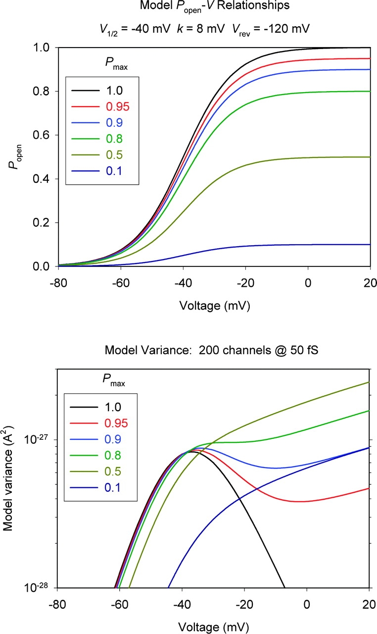
Model showing the voltage dependence of variance in a simple two-state channel, for different values of P _max, the maximum P _open during large depolarizations. The top panel shows the assumed P _open-V relationships with various P _max values, as indicated. All were calculated from a Boltzmann function with midpoint, V _1/2 = −40 mV and slope factor, k = 8 mV. The bottom panel shows the variance expected for 200 channels with γ_H 50 fS and V _rev −120 mV, assuming the various P _open-V relationships plotted above. The curves were generated using Eq. 1 with I _H = i _H N P _open = γ_H (V − V _rev) N P _open.

Ideally, the variance due to H⁺ channel gating, , would be measured under stationary conditions. At lower pH_i, the activation time course (turn-on) of H⁺ current was relatively rapid and accordingly these data appeared to be stationary. More rigorous tests of stationarity, in which the variance was estimated at different times during prolonged records also revealed no clear trends in σ². However, activation was much slower at pH_i 6.5, and up to several minutes were required at some voltages before stationarity was achieved. H⁺ current data that increased slowly during each successive record were “corrected” for the slow drift by subtracting a fitted single exponential curve. We discarded the first several records in which I _H increased more rapidly and used only the last few records, treating each one separately (i.e., with its own I _H, P _open, and ). In Fig. 1 (materials and methods) we showed empirically that measured during 12–20-s current records included >90% of the total that is expected to be obtained with much longer records.

Calculation of i_H from Stationary Variance of H⁺ Currents

Accepting that the current fluctuations originate in H⁺ channel gating, we would like to estimate the single channel H⁺ current, i _H, and related properties (the number of channels in the patch, N, and the open probability, P _open). i _H can be calculated from (Hille, 2001):

(1)

where is the H⁺ current variance, and I _H is the mean H⁺ current. Except for P _open, these parameters are directly measurable, although it is necessary to distinguish the contributions to current and variance that originate in H⁺ channels from background current or noise. The total σ² was essentially independent of voltage at subthreshold voltages where H⁺ channels are closed (Fig. 4). Therefore, we subtracted the average σ² at subthreshold voltages from that measured at voltages where H⁺ channels were open. This approach was used by Byerly and Suen (1989). Another approach is to inhibit H⁺ current with Zn²⁺ of Cd²⁺ and to consider the resulting σ² to be the background at that voltage (Bernheim et al., 1993). We avoided this approach because Zn²⁺ sometimes reduced both the background leak current and σ² at voltages where H⁺ channels were closed, and at high concentrations Zn²⁺ apparently caused membrane damage that increased σ² spuriously. In a few patches, the maximal H⁺ current was <1 pA and the fluctuations attributable to H⁺ channel gating were comparable with background levels (i.e., S/N ≈ 1). However, in most patches, S/N > 100, and sometimes S/N > 1,000, hence the subtraction of background variance had negligible effect. Determination of I _H required subtraction of leak current. Leak current at subthreshold voltages was usually Ohmic, and we extrapolated it to estimate the leak at each voltage where noise was measured. The most difficult parameter to estimate was P _open. In preliminary analyses, we approximated P _open as g _H measured during the noise record normalized to g _H,max from a family of pulses, which presumes that the maximum value of P _open (P _max) approaches 1.0 for large depolarizations. For measurements just above V _threshold where P _open is small, this assumption will cause only a small overestimation of i _H. However, knowledge of P _open becomes important at more positive voltages where g _H approaches saturation. For this reason, previous attempts to estimate i _H were restricted to voltages near V _threshold (Bernheim et al., 1993; DeCoursey and Cherny, 1993). Eventually, we adopted a procedure of data analysis (see below) that obviates the need to guess P _open.

What is the Limiting P_open at Large Depolarizations?

The calculation of i _H requires an estimate of P _open (Eq. 1). Although g _H may be proportional to P _open (after correction for rectification), it provides no information about P _max. However, the voltage dependence of the does provide evidence about P _max. Current fluctuations generate variance in proportion to the frequency of gating events, which is proportional to the product P _open(1-P _open) (Conti and Neher, 1980; Hille, 2001). Thus, gating transitions will occur most often and will be maximal near P _open = 0.5 (if P _max > 0.5). Fig. 5 (bottom) illustrates the voltage dependence of σ² calculated with a simple gating model using parameters typical of voltage-gated proton channels, assuming different values of P _max (Fig. 5, top). Although this heuristic model obviously ignores complexities of H⁺ channel gating, it describes the main features of the data remarkably well. If P _max is 1.0, σ² increases to a maximum near the midpoint of the g _H-V relationship and then decreases to 0 at large voltages where P _open → 1. If P _max is 0.1 or 0.5, the variance increases monotonically and almost linearly with depolarization (on a linear scale). If P _max is 0.8 there is a clear inflection, and if P _max is 0.9 the variance peaks and then decreases before increasing again. The P _max at which nonmonotonic -V behavior occurs depends somewhat on k, the slope factor of the g _H-V relationship. The appearance of these curves is also influenced by the relative positions of V _rev and the g _H-V relationship.

Comparison of the voltage dependence of actual σ² data (Fig. 4) with the model variance (Fig. 5) indicates that P _max ≥ ∼0.9 at low pH_i. In most patches studied at pH ≤ 5.5, reached a clear maximum with increasing depolarization, and then decreased before eventually increasing again. The maximum occurred near or slightly positive to V _1/2, indicated near the X axis in Fig. 4, precisely as expected from the simple model in Fig. 5. At pH_i 6.5, we did not see a clear maximum in , but usually a monotonic increase in with depolarization, although the increase was often more gradual during large depolarizations (i.e., positive to V _1/2 in Fig. 4). This behavior is suggestive of P _max ≤ 0.8. A more quantitative analysis of P _max is described in the next section.

Obtaining γ_H and N from a Linearized Plot of All Data

It is possible to obtain γ_H and N simultaneously without foreknowledge of P _open by plotting data obtained at multiple voltages in a simple format. From Sesti and Goldstein (1998):

(2)

where

(3)

Hence, provided γ _H is constant (e.g., no rectification) and N is constant (e.g., no rundown) a plot of y versus g _H should be linear. The Y intercept is the unitary conductance, γ _H, and the slope is −1/N. The intercept on the X axis is γ _H N, the maximum possible g _H if all channels were open simultaneously (which may be greater than the observed g _H,max). In practice, within the limits of experimental error, linear y-g_H plots were obtained, as in Fig. 6 . For pH_i 6.5, the slope was often small and sometimes not significantly different from zero. In such cases N could not be determined reliably, although γ_H could still be estimated.

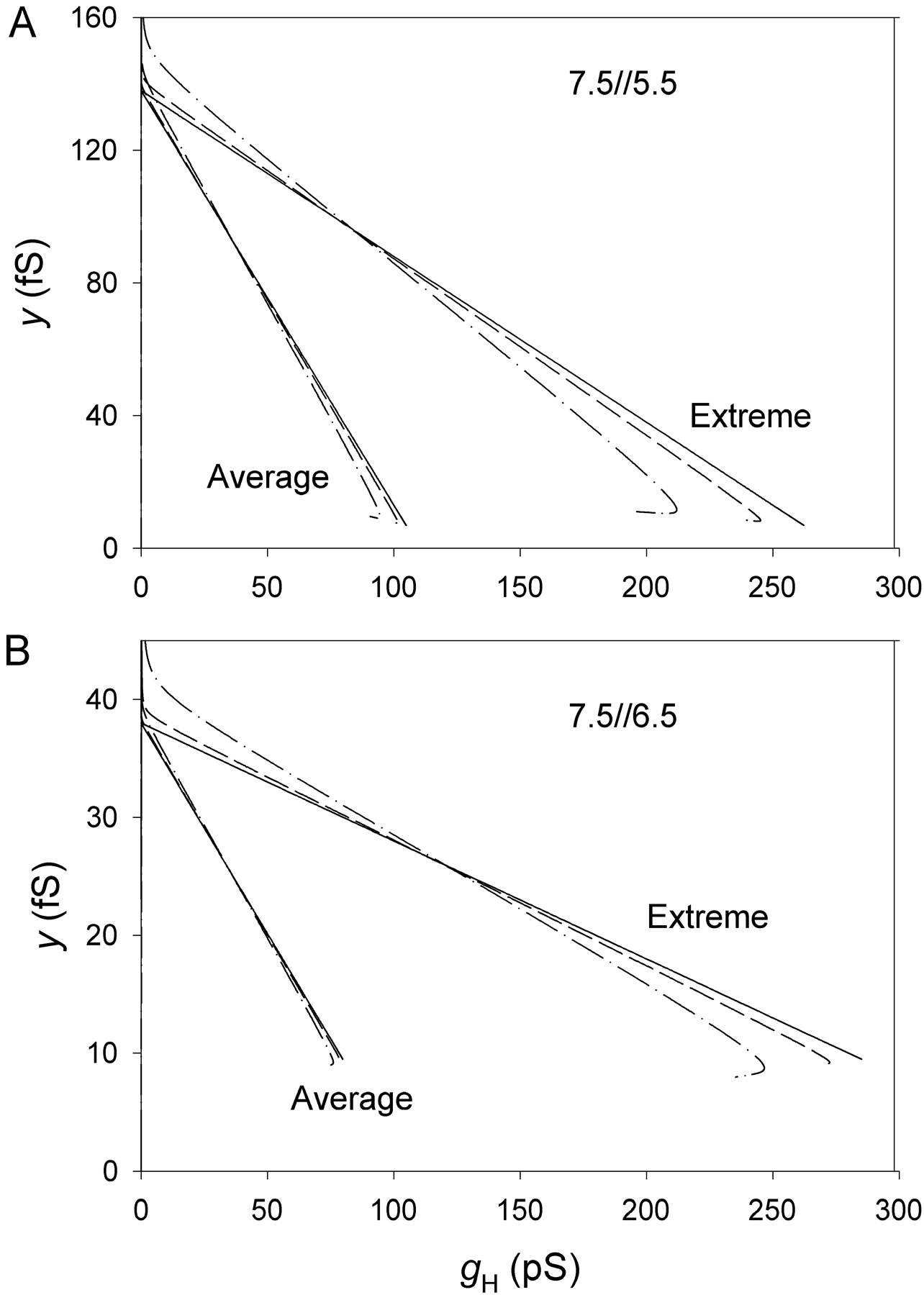
We adopted the y-g_H plot because (a) through N, it provides an estimate of P _open without requiring assuming an arbitrary value, and (b) it makes use of all the data over a range of voltages that include low to high P _open. Different errors are expected to occur at both extremes of P _open as well as at intermediate values. Near V _threshold, both I _H and σ² are close to background levels, and thus are poorly determined. During large depolarizations, i _H might be attenuated due to pH changes that result from prolonged H⁺ flux through the patch. This error is considered in the online supplemental material (available at http://www.jgp.org/cgi/content/full/jgp.200308813/DC1), and shown to have had little impact on the results. At intermediate voltages, the estimated I _H using Eq. 1 depends strongly on the limiting P _open value. Attempting to use Eq. 1 directly on individual records would require guessing P _open. By including all the data in plots such as in Fig. 6, we can estimate N, from which P _open can be calculated.

In Fig. 7 , P _open is plotted for the same patch as in other figures. To approach true steady-state, we plot only the estimate from the final record at each voltage. The results are quite similar to the simple g _H-V relationships in Fig. 3. The additional information obtained from Fig. 7 is the limiting value for P _open, P _max. Average values of P _max are given in Table I . Consistent with the behavior predicted from Figs. 4 and 5, P _max is 0.95 at pH_i ≤5.5, and at pH_i 6.5, P _max is 0.75. Almost all H⁺ channels open during large depolarizations at low pH_i, but P _max decreases at higher pH_i.

Figure 7.

Voltage dependence of P _open at pH_i 6.5, 5.5, and 5.0, for the same patch as in Figs. 2–4, and 6. P _open was estimated as g _H/(N γ _H), where the total number of channels in the patch, N, and γ_H were estimated from the y-g_H plot (Fig. 6). Here only the last 1–2 records at each voltage are included, because earlier points were farther from steady-state. Curves show best-fitting (by nonlinear least squares) Boltzmann functions: P _open = P _max {1 + exp[−(V − V _1/2)/k]}⁻¹ with midpoints (V _1/2) of −11.2, −26.9, and −42.9 mV, slope factors (k) of 5.7, 7.8, and 8.3 mV, and P _max of 0.78, 0.93, and 0.98 at pH_i 6.5, 5.5, and 5.0, respectively. ES-2596.

TABLE I.

Single H⁺ Channel Conductance (γ_H) and Maximum Open Probability (P_max) at Different pH

pHo//pHi	γH	P max
	mean ± SEM (n)	mean ± SEM (n)
	fS
7.5//6.5	37.4 ± 4.0 (19)	0.746 ± 0.027 (17)
6.5//6.5	38.3 ± 4.3 (3)	0.60 (1)
7.5//5.5	138.9 ± 7.5 (13)	0.954 ± 0.014 (10)
7.5//5.0	220 (2)	0.95 (2)
7.5//4.1	400 (1)	0.97 (1)

Estimates of γ_H and N were obtained from y-g_H plots (Fig. 6) and were based on the total H⁺ current variance (σ_H ²). If calculated using only the Lorentzian variance (σ_L ²), then the estimates of γ_H are about 20% lower, whereas the estimates of N are unaffected (Fig. 12).

The single-channel conductance, γ_H, is already determined from the y-g_H plot (Fig. 6). However, in Fig. 8 the unitary currents calculated for each noise sample are plotted. The lines are not fitted to these data but simply illustrate the values for γ_H obtained from the y-g_H plots. Single channel H⁺ currents are a few femtoamperes at pH_i 6.5, and increase markedly at lower pH_i. Mean values obtained for γ_H are given in Table I. Lowering pH_i from 6.5 to 5.5 increased γ_H by 3.7-fold on average. Although only a few measurements were made at pH 6.5//6.5, the similar γ_H obtained at pH 7.5//6.5 suggests that γ_H depends only on pH_i and not on pH_o.

Figure 8.

Single H⁺ channel current-voltage plots in the same patch and with the same symbol meanings as in Figs. 2–4 and 6 and 7. Estimates for i _H were obtained by using Eq. 1, where P _open is derived from the analysis in Fig. 7, and ultimately from the estimates of γ_H and N obtained from the y-g_H plot (Fig. 6). ES-2596.

Direct Measurement of Single-channel H⁺ Currents

Consistent with previous studies (Byerly and Suen, 1989; Bernheim et al., 1993; DeCoursey and Cherny, 1993), we were unable to detect single H⁺ channel currents directly when pH_i was 6.5 or higher. However, at pH_i 5.5 there were tiny step-like fluctuations in the current in some patches (Fig. 9) . Putative unitary currents could be resolved only near V _threshold, where just a few channels opened at a time. In Fig. 9, channel-like events are present at −60 and −70 mV, but at −50 mV too many channels are open to resolve discrete levels. The amplitude of the events at −60 mV is ∼10 fA, estimated as the difference in local mean current when the channel is judged to be open or closed. The analysis (y-g_H plot) of this patch indicated that i _H was ∼5 fA at −60 mV. Apparent single-channel currents in seven other patches under similar conditions were 7–16 fA, which is about twice as large as estimates obtained from variance analysis, although it is evident that the amplitudes are not clearly resolved. To our knowledge, these are the smallest single-channel currents identified by direct voltage-clamp measurement of any channel. Decker and Levitt (1988) resolved 25-fA H⁺ currents through gramicidin channels.

Figure 9.

Apparent single proton channel currents at pH_o 7.5 and pH_i 5.5. These currents were filtered at 20 Hz (8-pole Bessel) and later digitally refiltered at 10 Hz. The current scale is positioned arbitrarily. The resistance of this patch at subthreshold voltages was 5 TΩ. For clarity, each record is displaced vertically by 20 fA above its true position relative to the record underneath. ES2724.

Frequency Dependence of H⁺ Current Fluctuations

Power spectra were obtained from a subset of the data comprising 11 datasets from 7 different patches. Lorentzian spectral components could be identified under all pH regimes (Fig. 10) , although detection of the Lorentzian plateau was difficult for pH_i 6.5 (Fig. 10 B). The Lorentzian noise appeared to “turn on” when I _H became activated, and the variance contained within the Lorentzian component, (Fig. 11 , ▴), showed similar voltage dependence to the total current variance ( = open, = solid symbols in Fig. 4). Thus, the -V relationship exhibited a maximum for pH_i 5.0 and pH_i 5.5 (Fig. 11 A), but increased monotonically with V for pH_i 6.5 (Fig. 11 B). In addition to the Lorentzian noise, 1/f (Fig. 11, ○) and white noise (▾, Fig. 11) were also often observed. Both of these components increased monotonically with V. The 1/f component dominates at large depolarizing voltages because of the nonmonotonic voltage dependence of at low pH_i. For reference, the sum of the calculated shot noise of current flow and Johnson noise of the 50 GΩ feedback resistor in parallel with the patch resistance (Hainsworth et al., 1994), both of which are white noise, is shown by the dashed lines without symbols in Figs. 10 A and 11. The patch resistance was mainly determined by the H⁺ conductance. The 1/f spectrum at −80 mV in Fig. 10 A approaches this limiting noise level at ∼20 Hz.

Figure 10.

Power spectra of H⁺ current fluctuations. Test voltages (mV) are shown next to each curve. (A) pH_o = 7.5, pH_i = 5.5, V _threshold = −55 mV. The subthreshold data (▴) are fitted with a 1/f spectrum while the suprathreshold data sets are fitted with Lorentzian plus 1/f spectra. The latter two data sets can be fitted equally well by a Lorentzian plus white noise. The horizontal lines show the calculated sum of the spectral densities of the calculated shot noise of current flow and Johnson noise of the 50 GΩ feedback resistor in parallel with the patch resistance, which were: 3.8 × 10⁻³¹ (▴), 4.4 × 10⁻³¹ (○) and 1.7 × 10⁻³⁰ (▾) A² Hz⁻¹. (B) pH_o = 7.5, pH_i = 6.5, V _threshold < −30 mV. The near-threshold data (▴) are fitted with a Lorentzian plus white noise while the other datasets are each fitted with a Lorentzian plus 1/f plus white noise. The data at −10 and 20 mV can be fitted equally well with a 1/f spectrum plus white noise, but the exponents (m) on f are significantly greater than unity (1.29 ± 0.05 and 1.37 ± 0.07, respectively). The sum of Johnson- and shot-noise spectral densities were 1.3 × 10⁻³⁰ (▴), 8.4 × 10⁻³⁰ (○) and 2.0 × 10⁻²⁹ (▾) A² Hz⁻¹ (too small to show on this scale). Data in A and B are from two different patches (ES-2596, ES-2579).

If represents the only contribution of open/closed transitions to the current variance, then rather than should be used to estimate γ _H and N (Eqs. 2–3, Fig. 6). Fig. 12 illustrates y-g _H plots at pH_i 5.5 (A) or pH_i 6.5 (B), using either total H⁺ current variance (○) or only the integral of the Lorentzian component, (•). Surprisingly, γ _H and N were little affected when only the Lorentzian component was included. Estimates of γ _H based on σ_L ² were reduced by only ∼20% at all pH_i, and the estimates of N were, on average, unaffected for pH_i 5.0 and 5.5. The reason that estimates based only on are so similar to those based on is that σ_L ² dominates the total variance at small depolarizations. At large depolarizing voltages where the 1/f component becomes large (Fig. 11), and hence and diverge, the effect on the slope and intercept of the y-g _H plot is quite small.

Figure 12.

Examples of y-g _H plots with y calculated using the total variance (○, dashed line) or the Lorentzian variance (•, solid line). See Eqs 2 and 3. (A) pH_o 7.5, pH_i 5.5; (B) pH_o 7.5, pH_i 6.5. Same two patches as in Figs. 10 and 11. Regression lines were fitted after omitting the outliers near g _H = 0. In B, the slopes are not statistically significant, illustrating the difficulty of estimating N (= −1/slope) at pH_i 6.5. However, more reliable estimates of N were obtained in some cases (e.g., Fig. 6).

The Lorentzian time constants τ _L = (2π f _c)⁻¹ were smaller than the time constants for H⁺ current activation (τ _act) by roughly an order of magnitude (Fig. 13) . However, they showed a qualitatively similar dependence on pH_i. In contrast to τ _act (which decreases with V), no consistent voltage dependence could be discerned for τ _L, although this may have been masked by the considerable scatter. Mean deactivation time constants, τ _tail, measured during tail currents at voltages just negative to V _rev are plotted in Fig. 13. To compare τ _tail and τ _act with τ _L in the same voltage range, these measured τ _tail values are extrapolated to the midpoint voltage of the g _H-V relationship, assuming an exponential voltage dependence with a slope of 40 mV/e-fold change in τ _tail, as found in several studies (DeCoursey, 2003). The τ _L values are closer to τ _tail than to τ _act. At pH 7.5//5.5, we determined the mean open time in five patches in which apparently discrete events occurred near V _threshold (e.g., Fig. 9). The mean open time from these patches is similar to τ _L.

Figure 13.

Comparison of the Lorentzian time constants (τ _L), single-channel mean open times, and time constants of H⁺ current activation (τ _act) and deactivation (τ _tail) at various pH_o and pH_i. Mean open time is the global mean of data at −60 mV from five patches (n = 9–33 in each patch), estimated from current records like those in Fig. 9, in which apparently discrete single-channel events occurred near V _threshold, all filtered at 10–20 Hz. τ _act was determined by fitting the function I = I _max [1 − exp(−t/τ _act)] to I(t) curves such as those in Fig. 2 (top two panels). Mean values of τ _act for P _open = 0.5P _max are compared with mean values of τ _L (which showed no consistent dependence on P _open). Bars show standard errors from 2–4 patches; no error bars indicate only one patch was available. τ _tail at V < V _rev was determined by fitting a single exponential to tail currents recorded ∼10 mV negative to V _rev (mean ± SE, n = 8–18 for each pH). Also shown are τ _tail values extrapolated to the midpoint voltage of the g _H-V relationship, assuming exponential voltage dependence with a slope of 40 mV/e-fold change in τ _tail.

DISCUSSION

Proton Channel Gating Generates H⁺ Current Noise

Distinct H⁺ current fluctuations were clearly evident in patches of eosinophil membranes. Compelling evidence indicates that these fluctuations originate in the gating of voltage-gated proton channels. First, at various pH_i, σ² increases precisely at V _threshold. Second, σ² increases with voltage to a maximum that occurs near the midpoint of the g _H-V relationship at each pH_i. At larger depolarizing voltages, σ² then decreases at pH_i ≤ 5.5, but increases again gradually at very large depolarizing voltages. Precisely this behavior is predicted by a simple gating model to occur if P _max ≥ 0.9 (Fig. 5), but is exceedingly unlikely to result from fluctuations originating in leak current. Finally, no other conductance is evident under the ionic conditions of this study.

Single H⁺ channel currents were estimated from stationary and quasistationary H⁺ current variance, and were also measured directly at low pH_i. H⁺ current fluctuations could be resolved with excellent S/N because proton channels in mammalian cells, especially in phagocytes, gate at low frequencies (DeCoursey, 2003), which allows heavy filtering. In contrast, H⁺ current fluctuations could not be detected in snail neurons (Byerly and Suen, 1989), because these H⁺ channels open on a time-scale of a few milliseconds (Byerly et al., 1984), requiring ∼100-fold higher bandwidth. Bernheim et al. (1993) reported barely detectable excess H⁺ current noise in human skeletal myotubes, but they filtered at 5 kHz with S/N < 0.1. We previously detected distinct excess H⁺ current fluctuations in human neutrophils with 200 Hz but not 2 kHz lowpass filtering (DeCoursey and Cherny, 1993). Due to improved recording conditions and appropriate filtering, S/N is now typically ∼100, and in some patches as high as 2,000. At subthreshold voltages the variance was usually <10⁻²⁸ A², and sometimes as low as 2 × 10⁻²⁹ A², which is near the theoretical minimum noise level of 6.5 × 10⁻³⁰ A² for a patch-clamp recording setup with a 50 GΩ feedback resistor and a bandwidth of 20 Hz (Levis and Rae, 1993). The difference may be accounted for by 1/f noise of unknown origin (e.g., the spectrum at −80 mV in Fig. 10 A).

Power Spectra

A first order gating process should generate Lorentzian power spectra (Stevens, 1972). Power spectral analysis of voltage-gated proton current indicated a Lorentzian component whose voltage dependence coincided with that of H⁺ channel activation. Furthermore, the variance obtained as the integral of the Lorentzian component, , increased to a maximum near the midpoint of the g _H-V relationship and then decreased with further depolarization at pH_i ≤ 5.5, similar to the behavior of the total variance, . Thus, the Lorentzian component arises from H⁺ channel gating events. The Lorentzian time constants (τ _L) defined as τ _L = (2π f _c)⁻¹, were shorter than the time constants for proton-current activation (τ _act) by roughly an order of magnitude, but were in the range of τ _tail and the mean open time determined from single channel currents (Fig. 13).

In addition to a Lorentzian component, significant 1/f noise was also often observed. In contrast with Lorentzian spectra, the origin of this noise is unclear; 1/f noise can arise simply from nonstationary processes such as baseline drift (Conti et al., 1980). In the present study, the amplitude of 1/f noise became significant at voltages where I _H was activated (Fig. 11). Hence, at least part of the 1/f noise may have been associated with H⁺ conduction, or possibly even channel gating. Gating with distributed kinetics can generate 1/f noise (Sauvé and Szabo, 1985; Kogan, 1996; Bezrukov and Winterhalter, 2000). Similarly, the roll-off of a low frequency Lorentzian component might contribute low frequency variance that could be mistaken for 1/f noise. Excess white noise evident at high frequencies was also sometimes present (Fig. 11), although this component always represented only a small fraction of the total σ². White noise may have arisen in the recording system or could reflect an unresolved high frequency Lorentzian component.

It is possible that underestimates the current variance associated with channel gating. One or more Lorentzian components at low frequencies may not have been detected, or were interpreted as 1/f noise. A Lorentzian with a corner frequency (f _c) corresponding to the time constant of H⁺ current activation (τ _act) is to be expected (Colquhoun and Hawkes, 1977), but could have been resolved only at low pH_i. At pH_i 6.5, clear resolution of such a Lorentzian component (i.e., resolution down to f _c/10) would require stationary current samples ∼70 min long. Similarly, if all or part of the 1/f noise were associated with channel gating (e.g., if the 1/f spectrum were actually a superposition of Lorentzians) then estimates of γ _H based on (Fig. 12) will be downwardly biased. The same can be said of the white noise component, although this was very small. On average, however, the estimates of γ _H based on and differ by only ∼20%.

Unitary H⁺ Currents Increase at Low pH_i More Than Macroscopic Conductance

The single channel conductance estimated from was 38 fS at pH_i 6.5, and 139 fS at pH_i 5.5 (Table I). A few measurements at lower pH_i (where patches were extremely unstable) indicate similar pH_i dependence. Extrapolating γ_H at pH_i 5.5 and 6.5 to pH_i 7.2 gives an estimate of 15 fS for the unitary conductance at physiological pH. Corrected to 37°C assuming a Q ₁₀ of 2.8 (DeCoursey and Cherny, 1998), γ_H becomes 78 fS. The most surprising result of this study was that the single channel conductance increased 3.7-fold at pH_i 5.5 compared with pH_i 6.5, in contrast with the macroscopic conductance, which increased only 1.8-fold. In nearly all existing studies of voltage-gated proton channels, the macroscopic g _H increased only ∼2-fold per unit decrease in pH_i (DeCoursey, 2003). The relative pH independence of the macroscopic g _H has been considered somewhat paradoxical, both for voltage-gated proton channels (DeCoursey and Cherny, 1994) and for the proton channel of ATP synthase (Junge, 1989). In contrast, the H⁺ conductance of gramicidin channels is almost directly proportional to [H⁺] over a wide pH range (Eisenman et al., 1980; DeCoursey, 2003). The unitary conductance found here (Table I) is not proportional to [H⁺], but is closer to proportionality than estimates based on macroscopic g _H measurements.

Because lowering pH_i increased the estimated single-channel conductance substantially more than the macroscopic g _H,max, the total number of H⁺ channels, N, must decrease. This anomalous behavior has several possible explanations. Although the result might be artifactual, consideration of possible sources of error does not lead to likely candidates. The variance at higher pH_i might be underestimated if we did not sample a sufficiently low frequency range, but the variance-versus-record length analysis (materials and methods) gave no indication of this. Progressive rundown (loss of functioning channels) at lower pH_i could contribute in experiments in which measurements were first made at higher pH_i. However, correction for rundown or reversing the order of pH_i measurements did not eliminate the phenomenon. The observed pH_i dependence of P _max does not explain this result, but instead works in the opposite direction. There seems no alternative but to accept that low pH_i actually reduces the number of functioning H⁺ channels. Based on the average values of γ_H, P _max, and g _H, N is 2.6 greater at pH_i 6.5 than 5.5 (or 62% of the channels at pH_i 6.5 are unavailable at pH_i 5.5).

Single-channel–like events (7–16 fA) could be observed directly in many patches at pH_i ≤ 5.5, just above V _threshold. The amplitude of these events was not well-resolved, but usually was about double the unitary H⁺ current calculated at the same voltage from . It is possible that these events were simultaneous openings of multiple channels, and that the single channels were simply not resolved. Alternatively, H⁺ channels may have a cooperative gating mechanism. We assume that most H⁺ current fluctuations occur within the frequency range examined. The adequacy of the bandwidth employed in the low frequency range was demonstrated empirically in Fig. 1, but it is possible that there could be components of gating at higher frequencies than we explored. Of course, it is possible that the discrepancy simply reflects errors in the measurements.

If each channel flickered on a millisecond scale, we would have resolved only the average current. However, from the vantage point of most cellular processes, such as pH_i regulation, a channel that conducts 5 fA of continuous H⁺ current is functionally equivalent to one that conducts 10 fA but flickers rapidly with P _open = 0.5.

Judged solely by their conductance, voltage-gated proton channels cannot be distinguished conclusively from highly efficient carriers. For example, H⁺ efflux through Na⁺/H⁺-antiporters in human fibroblasts at their maximum turnover rate at pH_i 6.0 is equivalent to 0.5–1.7 fA (Siczkowski et al., 1994). Present estimates of γ_H correspond with transport of 2.4 × 10⁴ H⁺/s (3.8 fA) at pH_i 6.5 for a 100-mV driving force, and 9 × 10⁴ H⁺/s (14 fA) at pH_i 5.5. Although the conductance of H⁺ channels is very small compared with other ion channels, in view of the low concentration of protons at physiological pH, the conductance is, if anything, larger than expected. Gramicidin channels can conduct >2 × 10⁹ H⁺/s (Cukierman, 2000) at pH < 0, which is a higher rate than any other selective ion channel conducts any ion. The g _H of gramicidin channels is directly proportional to [H⁺] over a wide pH range (DeCoursey, 2003). However, extrapolation of this pH dependence to pH_i 6 predicts <1 fA of H⁺ current at 100 mV. The present demonstration of distinct H⁺ current fluctuations attributable to voltage- and pH-dependent gating confirms that voltage-gated proton channels behave like genuine ion channels, in spite of their conductance at physiological pH being low enough to approach the range of carriers. Voltage-gated proton channels are simply channels with a small conductance.

References

- Benndorf, K. 1994. Properties of single cardiac Na channels at 35°C. J. Gen. Physiol. 104:801–820. [DOI] [PMC free article] [PubMed] [Google Scholar]
- Bernheim, L., R.M. Krause, A. Baroffio, M. Hamann, A. Kaelin, and C.-R. Bader. 1993. A voltage-dependent proton current in cultured human skeletal muscle myotubes. J. Physiol. 470:313–333. [DOI] [PMC free article] [PubMed] [Google Scholar]
- Bezrukov, S.M., and M. Winterhalter. 2000. Examining noise sources at the single-molecule level: 1/f noise of an open maltoporin channel. Phys. Rev. Lett. 85:202–205. [DOI] [PubMed] [Google Scholar]
- Byerly, L., R. Meech, and W. Moody. 1984. Rapidly activating hydrogen ion currents in perfused neurones of the snail, Lymnaea stagnalis. J. Physiol. 351:199–216. [DOI] [PMC free article] [PubMed] [Google Scholar]
- Byerly, L., and Y. Suen. 1989. Characterization of proton currents in neurones of the snail, Lymnaea stagnalis. J. Physiol. 413:75–89. [DOI] [PMC free article] [PubMed] [Google Scholar]
- Cherny, V.V., L.L. Thomas, and T.E. DeCoursey. 2001. Voltage-gated proton currents in human basophils. Biologicheskie Membrany. 18:458–465. [Google Scholar]
- Cherny, V.V., R. Murphy, and T.E. DeCoursey. 2002. Single proton channel currents are really small. Biophys. J. 82:639a. [Google Scholar]
- Colquhoun, D., and A.G. Hawkes. 1977. Relaxation and fluctuations of membrane currents that flow through drug-operated channels. Proc. R. Soc. Lond. B Biol. Sci. 199:231–262. [DOI] [PubMed] [Google Scholar]
- Conti, F., L.J. De Felice, and E. Wanke. 1975. Potassium and sodium ion current noise in the membrane of the squid giant axon. J. Physiol. 248:45–82. [DOI] [PMC free article] [PubMed] [Google Scholar]
- Conti, F., and E. Neher. 1980. Single channel recordings of K+ currents in squid axons. Nature. 285:140–143. [DOI] [PubMed] [Google Scholar]
- Conti, F., B. Neumcke, W. Nonner, and R. Stämpfli. 1980. Conductance fluctuations from the inactivation process of sodium channels in myelinated nerve fibres. J. Physiol. 308:217–239. [DOI] [PMC free article] [PubMed] [Google Scholar]
- Cukierman, S. 2000. Proton mobilities in water and in different stereoisomers of covalently linked gramicidin A channels. Biophys. J. 78:1825–1834. [DOI] [PMC free article] [PubMed] [Google Scholar]
- Decker, E.R., and D.G. Levitt. 1988. Use of weak acids to determine the bulk diffusion limitation of H+ ion conductance through the gramicidin channel. Biophys. J. 53:25–32. [DOI] [PMC free article] [PubMed] [Google Scholar]
- DeCoursey, T.E. 1991. Hydrogen ion currents in rat alveolar epithelial cells. Biophys. J. 60:1243–1253. [DOI] [PMC free article] [PubMed] [Google Scholar]
- DeCoursey, T.E. 2003. Voltage-gated proton channels and other proton transfer pathways. Physiol. Rev. 83:475–579. [DOI] [PubMed] [Google Scholar]
- DeCoursey, T.E., and V.V. Cherny. 1993. Potential, pH, and arachidonate gate hydrogen ion currents in human neutrophils. Biophys. J. 65:1590–1598. [DOI] [PMC free article] [PubMed] [Google Scholar]
- DeCoursey, T.E., and V.V. Cherny. 1994. Voltage-activated hydrogen ion currents. J. Membr. Biol. 141:203–223. [DOI] [PubMed] [Google Scholar]
- DeCoursey, T.E., and V.V. Cherny. 1997. Deuterium isotope effects on permeation and gating of proton channels in rat alveolar epithelium. J. Gen. Physiol. 109:415–434. [DOI] [PMC free article] [PubMed] [Google Scholar]
- DeCoursey, T.E., and V.V. Cherny. 1998. Temperature dependence of voltage-gated H+ currents in human neutrophils, rat alveolar epithelial cells, and mammalian phagocytes. J. Gen. Physiol. 112:503–522. [DOI] [PMC free article] [PubMed] [Google Scholar]
- DeCoursey, T.E., J. Dempster, and O.F. Hutter. 1984. Inward rectifier current noise in frog skeletal muscle. J. Physiol. 349:299–327. [DOI] [PMC free article] [PubMed] [Google Scholar]
- DeCoursey, T.E., V.V. Cherny, A.G. DeCoursey, W. Xu, and L.L. Thomas. 2001. Interactions between NADPH oxidase-related proton and electron currents in human eosinophils. J. Physiol. 535:767–781. [DOI] [PMC free article] [PubMed] [Google Scholar]
- DeFelice, L.J. 1981. Introduction to Membrane Noise. Plenum Press, New York. 500 pp.
- Diggle, P.J. 1990. Time Series: A Biostatistical Introduction. Clarendon Press, Oxford. 257 pp.
- Eisenman, G., B. Enos, J. Hägglund, and J. Sandblom. 1980. Gramicidin as an example of a single-filing ionic channel. Ann. NY Acad. Sci. 339:8–20. [DOI] [PubMed] [Google Scholar]
- Gallant, A.R. 1975. Nonlinear regression. The American Statistician. 29:73–81. [Google Scholar]
- Hainsworth, A.H., R.A. Levis, and R.S. Eisenberg. 1994. Origins of open-channel noise in the large potassium channel of sarcoplasmic reticulum. J. Gen. Physiol. 104:857–883. [DOI] [PMC free article] [PubMed] [Google Scholar]
- Hille, B. 2001. Ion Channels of Excitable Membranes. Third edition. Sinauer Associates, Inc., Sunderland, MA. 814 pp.
- Junge, W. 1989. Protons, the thylakoid membrane, and the chloroplast ATP synthase. Ann. NY Acad. Sci. 574:268–285. [DOI] [PubMed] [Google Scholar]
- Kogan, Sh. 1996. Electronic Noise and Fluctuations in Solids. Cambridge University Press. 354 pp.
- Kuno, M., J. Kawawaki, and F. Nakamura. 1997. A highly temperature-sensitive proton conductance in mouse bone marrow-derived mast cells. J. Gen. Physiol. 109:731–740. [DOI] [PMC free article] [PubMed] [Google Scholar]
- Levis, R.A., and J.L. Rae. 1993. The use of quartz patch pipettes for low noise single channel recording. Biophys. J. 65:1666–1677. [DOI] [PMC free article] [PubMed] [Google Scholar]
- Murphy, R., V.V. Cherny, V. Sokolov, and T.E. DeCoursey. 2003. Power spectral analysis of voltage-gated proton current noise in human eosinophils. Biophys. J. 84:556a. [Google Scholar]
- Nagle, J.F., and H.J. Morowitz. 1978. Molecular mechanisms for proton transport in membranes. Proc. Natl. Acad. Sci. USA. 75:298–302. [DOI] [PMC free article] [PubMed] [Google Scholar]
- Neumcke, B. 1978. 1/f noise in membranes. Biophys. Struct. Mech. 4:179–199. [DOI] [PubMed] [Google Scholar]
- Otnes, R.K., and L. Enochson. 1978. Applied Time Series Analysis. John Wiley and Sons, New York. 449 pp.
- Press, W.H., S.A. Teukolsky, W.T. Vetterling, and B.P. Flannery. 1992. Numerical Recipes in FORTRAN: The Art of Scientific Computing. Cambridge University Press. 963 pp.
- Sauvé, R., and G. Szabo. 1985. Interpretation of 1/f fluctuations in ion conducting membranes. J. Theor. Biol. 113:501–516. [DOI] [PubMed] [Google Scholar]
- Sesti, F., and S.A. Goldstein. 1998. Single-channel characteristics of wild-type IKs channels and channels formed with two minK mutants that cause long QT syndrome. J. Gen. Physiol. 112:651–663. [DOI] [PMC free article] [PubMed] [Google Scholar]
- Siczkowski, M., J.E. Davies, and L.L. Ng. 1994. Activity and density of the Na+-H+ antiporter in normal and transformed human lymphocytes and fibroblasts. Am. J. Physiol. 267:C745–C752. [DOI] [PubMed] [Google Scholar]
- Stevens, C.F. 1972. Inferences about membrane properties from electrical noise measurements. Biophys. J. 12:1028–1047. [DOI] [PMC free article] [PubMed] [Google Scholar]
- Thomas, R.C., and R.W. Meech. 1982. Hydrogen ion currents and intracellular pH in depolarized voltage-clamped snail neurones. Nature. 299:826–828. [DOI] [PubMed] [Google Scholar]
- Tietze, U., and Ch. Schenk. 1978. Advanced Electronic Circuits. Springer-Verlag, Berlin. 510 pp.
- Walpole, R.E., and R.H. Myers. 1978. Probability and Statistics for Engineers and Scientists. Macmillan Publishing Co. Inc., New York. 580 pp.
Associated Data
This section collects any data citations, data availability statements, or supplementary materials included in this article.