Selection Against Demographic Stochasticity in Age-Structured Populations

Abstract

It has been shown that differences in fecundity variance can influence the probability of invasion of a genotype in a population; i.e., a genotype with lower variance in offspring number can be favored in finite populations even if it has a somewhat lower mean fitness than a competitor. In this article, Gillespie's results are extended to population genetic systems with explicit age structure, where the demographic variance (variance in growth rate) calculated in the work of Engen and colleagues is used as a generalization of “variance in offspring number” to predict the interaction between deterministic and random forces driving change in allele frequency. By calculating the variance from the life-history parameters, it is shown that selection against variance in the growth rate will favor a genotypes with lower stochasticity in age-specific survival and fertility rates. A diffusion approximation for selection and drift in a population with two genotypes with different life-history matrices (and therefore different mean growth rates and demographic variances) is derived and shown to be consistent with individual-based simulations. It is also argued that for finite populations, perturbation analyses of both the mean and the variance in growth rate may be necessary to determine the sensitivity of fitness to changes in the life-history parameters.

THEORETICAL population genetics deals primarily with furthering the understanding of how stochastic and deterministic factors interact to drive change in gene frequency p in a population. The deterministic force in question is usually natural selection (on survivorship, fecundity, etc.) while the stochasticity can arise from either extrinsic or intrinsic forces. In the former case, it can be due to fluctuating environmental conditions (Haldane and Jayakar 1963; Lewontin and Cohen 1969; Turelli 1977; Tuljapurkar and Orzack 1980) or to the familiar process of finite sampling of gametes from a large gamete pool that leads to the standard scenarios of genetic drift (e.g., Wright 1931; Kimura 1964). In contrast, intrinsic variance in fecundity arises from the fact that survival and reproductive output are themselves probabilistic events, where even in a constant environment, a given genotype will not produce a fixed number of offspring or survive until the same age. This article focuses specifically on the intrinsic fecundity variance and its generation as demographic variance in age-structured systems.

Gillespie (1974) investigated the role of intrinsic variance in fecundity, showing that the contribution of this variance to the change in allele frequency arises as a consequence of sampling from a finite gamete pool, as opposed to sampling of gametes from an effectively infinite gamete pool in Fisher–Wright–Kimura models of genetic drift. For a finite gamete pool, if the distribution of fecundities among individuals of a given genotype is non-Poisson, the sample variance in gamete frequencies induces changes in gametic frequencies across generations (Gillespie 1975; Rousset and Ronce 2004; Lehmann and Balloux 2007). Gillespie's results demonstrated that in a finite population, the fecundity variance contributes to both the first and the second moments of Δp = p(t + 1) − p(t). This is in contrast to the genetic drift that arises from sampling from an infinite gamete pool (classical genetic drift) or from samples of a gamete pool where the distribution of individual fecundities is Poisson. Under these scenarios, variance in fecundity does not influence E[Δp] but only the expectation of second moments E[(Δp)²].

Consider two competing asexual haploid genotypes in a population size N. Following Gillespie here and elsewhere in the text, we define the fecundity as the number of offspring produced by a given genotype prior to density regulation (culling to maintain a constant population size). It is assumed that the fecundity of a given genotype can be characterized by the mean and variance alone and that the magnitude of the variance is greater than that of the mean (i.e., greater than Poisson). The respective mean and variance of the fecundities μ₁, μ₂, , give, to a first-order approximation when the variances are small and the averages are near unity,

(1a)

(1b)

(see also Proulx 2000, for derivations of these expressions).

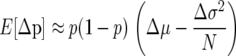
It can be seen from (1a) that in a finite population, directional selection will favor reduced offspring number (fecundity) variance by tending to increase the frequency of genotypes with lower σ²-values. In particular, when the mean fitness differences are relatively small, selection will tend to favor the genotype with lower variance. In fact, selection can actually favor a genotype with lower average fitness if it sufficiently reduces the variance; i.e., when 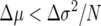, the allele with lower variance will have a higher than neutral probability of fixation. Intuitively, the fact that fixation probabilities depend on the variance as well as the first moment in fitness can be understood from the standpoint of “bet hedging” (Seger and Brockman 1987; Stearns 2000). Even if the mean fitness is high, a high variance value will lead to few (or no) offspring in some generations, thus leading to lineage extinction. This effect is more pronounced in a small population (since variance in a sample mean parameter scales inversely with sample size N), since for N large at least some individuals are likely to compensate with many offspring for those that have few.

Under the assumptions of weak selection and low variance, (1a) and (1b) can be used, respectively, to approximate the drift and diffusion coefficients in the Kolmogorov backward equations. These give estimates for fixation probabilities of a given genotype when the only source of stochasticity is intrinsic; i.e.,

(2)

which is independent of population size when the mean fitness difference is 0. The predictions of the diffusion approximation for selection on fertility variance are consistent with simulation results (Gillespie 1974; Shpak 2005). Strictly speaking, the above expression is an approximation, based on a continuous-time diffusion representation of (1). As such, it requires that μ ≈ 1 + r with r small for both genotypes, since a representation in continuous rather than discrete time is in terms of log-scale transformations of the parameters (see below), with r = Log[μ] in place of μ and σ²/μ² as the variance term to give appropriate scaling of the variance terms.

Gillespie's presentation of selection on variance in offspring number does not deal explicitly with age structure (i.e., in the derivations, there is effectively a single age class with variance in fertility) or any other life-history variable. In his studies, it was assumed that the number of offspring contributed by a genotype was a random variable described as μ + δ, where δ was a random variable with variance σ². The variance would arise as a consequence of the genotype undertaking different life-history “strategies,” although the variance was never explicitly derived in these terms. A formal derivation of variance in fitness for organisms selecting different strategies or environments was given by Demetrius and Gundlach (2000), which was the first treatment that explicitly calculated variance from life-history variables rather than assuming it to be a given value.

Gillespie originally formulated the problem so that age structure could be (implicitly) a source of fecundity variance, even though this was not formally derived. In Gillespie (1974), divergent variances in offspring number were proposed to arise from semelparous vs. iteroparous life histories. Specifically, one genotype produces a single clutch of k offspring that survive or die (collectively) with probability π, while another produces k individual offspring at different points, each of which survives individually with probability π. While both strategies have the same expected number of offspring, E[x] = kπ, the variance in surviving offspring number in the former, semelparous case is Var[x] = k²π(1 − π) vs. the smaller kπ(1 − π) in the iteroparous scenario.

Substituting these binomial variance values into Equations 1 and 2 gives an estimate of fixation probabilities that is in close agreement with the frequencies of fixation or loss in individual-based simulations of these life histories under a variety of conditions (Shpak 2005), at least for relatively small selection coefficients. However, it should be apparent that substituting these values is only an approximation, in that it reduces an evolutionary model with age structure (for the iteroparous individual) to a unidimensional one without age classes. Consequently, selective dynamics driven by differences in generation time or in reproductive value contributions from each age class (under potentially different distributions) are ignored, with potentially misleading results. For a complete understanding of how selection for variance in offspring number operates, the variance terms must be calculated explicitly from models with age structure. In the simple example of semelparity and iteroparity outlined above as in more general models, the variance can be derived from Leslie matrix representations.

There is extensive literature on describing selection dynamics in age-structured populations (e.g., Charlesworth 1994 for a review), along with some articles dealing with diffusion approximations in such systems. Most of these models assume either a very large population size or a Poisson distribution of fecundities, in which case terms other than the first moment of growth rate (or of the Malthusian parameter on a log scale) can be neglected in calculating the selection coefficients; i.e., the sign of Δλ calculated from the Leslie matrices of two genotypes is sufficient to determine which one has a higher probability of fixation. Such models are entirely analogous to classical population genetic models without age structure prior to the introduction of Gillespie's results.

A number of workers have gone beyond the first-moment approximation to the Malthusian parameter. Demetrius and colleagues (Demetrius and Gundlach 1999; Demetrius and Ziehe 2007) derived diffusion equations for selection on genotypes in age-structured populations where contributions of the second and higher moments in growth rate appear in the diffusion and drift coefficients. The equations they derived, in terms of first and second moments, had the same form as in Equations 1 and 2. However, the form of stochasticity that they considered was quite different from the stochasticity that arises as a consequence of intrinsic variance in fecundity and in survival rates. Their variance term arises instead from genealogical stochasticity, i.e., the probability distribution describing what age class contributes an offspring. As such, their work addresses a different problem that is not an age-structured generalization of Gillespie's results.

Leturque and Rousset (2002) and Rousset and Ronce (2004) derived general expressions for selection coefficients in any type of class-structured population, in which the variance and higher moments of growth rate could arise from stochasticity in fecundity, survivorship, or migration. Nevertheless, for these expressions to be computationally tractable, it was again necessary to posit a Poisson distribution of fecundities, which gives selection equations in which fecundity variance terms are absent.

The first explicit attempt at characterizing selection coefficients in a closed form in terms of first and second moments when the distribution of fecundities and survivorship is arbitrary (variances greater than Poisson) was undertaken by Steinar Engen, Russell Lande, and their colleagues (e.g., Lande et al. 2003). Much of their work focuses on the stochastic dynamics of a single genotype in the context of calculating extinction probabilities.

In what follows, it is shown that the variance calculations from life-history matrices can be used directly as terms in (1) and (2), generalizing the Gillespie equations to selection on fecundity and survival variance in age-structured populations. In the first section, the results of Steinar Engen and colleagues on the calculation of demographic variances are recapitulated. Subsequent sections extend their results to describe competition between two genotypes, in which demographic variance induced by Leslie matrices determines which genotype will have a higher probability of fixation, which in turn is validated with simulations. In the discussion, it is proposed that sensitivity analysis of demographic variance may be as important a determinant of the response of selection to changes in life-history traits as sensitivity analysis of the growth rate's first moment.

DEMOGRAPHIC VARIANCE IN AGE-STRUCTURED POPULATIONS

For a vector n = {n₁, … , n_d} describing the number of individual x_i in the ith age class, the number of individuals in the next time step can be predicted from the fecundities and survival frequencies of each class. Leslie (1945) introduced a matrix representation such that n(t + 1) = Ln(t),

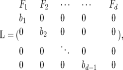where F_i is the fertility of the ith age class and b_i is the fraction of individuals in that class that survive to the next time step. Treated as a deterministic dynamical system where the parameters are rates, the population dynamics and evolution of age-structured systems are well studied and understood (e.g., Charlesworth 1994; Caswell 2001). Much of the theory is based on an understanding of the eigenstructure of L, where the leading eigenvalue λ gives the growth rate when the age class distribution is close to the frequencies given by the corresponding eigenvector. This is done under the assumption that the coefficients of L are deterministic (constant valued).

However, a strictly deterministic interpretation of the Leslie matrix obscures the fact that the parameters b and F are actually random variables (so that deterministic models based on Leslie matrices actually use the mean values and as their coefficients for each age class parameter), and, by definition, the leading eigenvalue (growth rate λ) is itself a random variable. We thus distinguish between the growth rate λ of L and its expectation E[λ] = μ, which corresponds to the growth rate (first eigenvalue) of a matrix E[L] where the coefficients are the expected values of each value L_ij. Similarly, we distinguish between the Malthusian parameter of the random matrix ρ = Log[λ] and its expectation r = Log[μ].

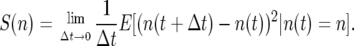
In natural populations, it is not a fixed fraction b_i of individuals that survive to the i + 1 age class, because survival of any individual from year to year is itself probabilistic. Rather, b_i is a Bernoulli probability with mean b_i and variance b_i(1 − b_i). This in turn implies that the number of survivors in the next age class of a pool of n_i will have a binomial distribution with mean n_ib_i and variance n_ib_i(1 − b_i), while the variance in the fraction of survivors is b_i(1 − b_i)/n_i. The fertility values in any given age class F_i are also (often) themselves random variables, since the reproductive output of a given age class (even holding the genotype constant) is seldom fixed. If the census point of the population is taken prior to reproduction, the fertility of an age class is the product of that age class's fecundity m_i multiplied by the probability of surviving through to the end of the first age class; i.e., F_i = b_om_i. Thus, even when m_i is assumed constant, there is again a contribution from the Bernoulli variance b_o(1 − b_o) of survival probabilities (Caswell 2001).

If m_i is itself a random variable (which can follow virtually any probability distribution, characterized by mean m_i and variance ), one has true fecundity variance (variance in offspring number prior to culling), and in the limiting case of a single age class, one has the variance quantity seen in Gillespie (1975), where is the variance term in (1) and (2). Note that in an age-structured population, it is not accurate to describe the variance that arises from differential survivorship across age classes as “variance in offspring number” and to use it as anything but an approximation in Gillespie's equations. To correctly describe selection on variance in age-structured populations in terms of a single variance parameter, one needs to calculate not the variance in offspring number (fecundity) but the rather variance in the population growth rate λ.

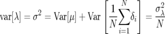
This quantity, referred to as demographic variance, has been derived and discussed in detail in the works of Steinar Engen and co-workers (e.g., Engen et al. 2005a,b). The perturbation of λ proposed by Tuljapurkar (1982, see also Caswell 2001, Chap. 14) to calculate the environmental variance term applies to calculations of the demographic variance (Lande et al. 2003). One can write λ = μ + δ, where μ = E[λ] is the expected growth rate and δ is a random variable with mean 0 and a variance of . In a population of N individuals, variation in growth rate is due to the variance of the sample mean; i.e.,

(3)

(since μ is a constant).

With population size on a log scale X = log[N], the mean growth rate r = log[λ], which from a Taylor expansion of r about the mean μ gives the expectation

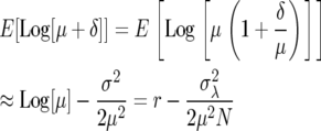(4)

(here σ² is the variance in sample mean growth rate, which is simply the demographic variance /N). Higher-order terms can be neglected when deviations from the mean are relatively small (i.e., δ/μ < 1) or when the distribution of fecundities is characterized by first and second moments alone (as would be the case for a number of distributions).

For a single genotype, the growth rate in a finite population is estimated as the difference between mean growth rate and the (suitably scaled) demographic variance divided by population size. It is seen below that in competition between different genotypes this will be the relevant measure of fitness.

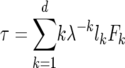
The demographic variance, in turn, can be calculated directly from the Leslie matrix parameters when one assumes that F_i and b_i are themselves random variables. To calculate the variance of λ, we note that for any function f(x₁, x₂, … , x_k) of random variables x_i, the variance of f(x) up to second-order approximation is given by

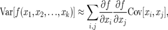which in the absence of covariances between parameters is

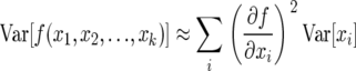(e.g., Tiwari and Elston 1999).

Since the leading eigenvalue is a function of the Leslie matrix parameters x_i, the variance in λ can be estimated as

(5)

because the variance of interest is the sample variance of the gamete pool, Var[x_i] = Var[δ_i]/n_i, where n_i is the number of individuals in the ith class and δ_i is the random variable component of the ith parameter (Lande et al. 2003, p. 64).

The relevant parameters are , . If survival of each individual in an age class is assumed to be a Bernoulli random variable, var(b_i) = b_i(1 − b_i), while the variance in F_i is the combined contribution of variance in offspring number m_i and the survival probability from birth to the first age class p₀. For a population in age class equilibrium , the variance of the sample mean contribution of each age class parameter, n_i is the product of census population size and the equilibrium frequency of the ith age class, N∨_i.

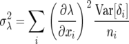
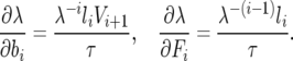
Furthermore, the partial derivatives of the growth rate with respect to the life-history parameters have been calculated (as proposed in Hamilton 1966 and Demetrius 1969, and elaborated in Caswell 2001) as

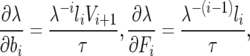where l_i is the probability of survival to age class i, , while τ and V refer, respectively, to the expected generation time of a life history specified by Leslie matrix L and the reproductive value (sensu Fisher 1958) of an individual in the ith age class (i.e., the expected number of progeny of an individual in age i from the present time until its death). These quantities are

Putting the above expressions together, one has an estimate for demographic variance that can be calculated directly from the life-history parameters:

(6)

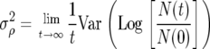
(Engen et al. 2005a,b). On the logarithmic scale, the demographic variance is .

It was demonstrated by Engen et al. (2007) that strictly speaking, the above growth and variance terms do not necessarily describe first and second moments in the population growth rate from one generation to the next (with population size defined as the census number of individuals). Rather, the growth rate λ determines the rate of increase in the population reproductive value, which is given by V = V.n (where V is the vector of reproductive values and n a vector describing the number of individuals in each age class), and from the fact that the distribution of reproductive values is the left eigenvector of L, we have E[V(t + 1) | V(t)] = λV(t). Because of the stochasticity inherent in the survival and reproductive processes, the distribution of age classes from one time step to the next will deviate from the stable age frequency ν. This deviation is especially evident when the generation time of the life history is significantly longer than a single time step (Engen et al. 2007).

As a result, the mean and the variance of λ will only approximately describe the first and second moments in N(t) from one time step to the next. While the expected growth rate of N(t) is the same as that for V(t), the variance of the former will actually be

(7)

i.e., the variance contribution of each age class weighted by its frequency near equilibrium. It can be seen that Equation 7 corresponds closely with (6) only when τ ≈ 1 and when the reproductive value is approximately equal to the fertility of the age class in question. However, over multiple time steps (t ≫ τ), the approximation N(t) ≈ λ^tV(0) ≈ λ^tN(0). Consequently, demographic variance of reproductive value can be used as a reliable estimate for the second moment of population growth rate given sufficient time.

In formal terms, the convergence of first and second moments in population growth rate to the dynamics of reproductive value is given by

The approximation of mean and variance in reproductive value growth rate describing the first and second moments in population number is useful for a number of reasons. First, population census number is easier to estimate than population reproductive value. More importantly, describing the system in terms of N(t) is critical for deriving equations describing competition between two genotypes with different life-history parameters.

The variances in Equations 6 and 7 induced by a general (non-Poisson) distribution of fecundity and Bernoulli survival probabilities suggest that selection equations and diffusion approximations that do not make use of demographic variances may lead to misleading conclusions in general cases. In contrast, the selection coefficients derived from first- and second-moment approximations to growth rates of stochastic Leslie matrices allow one to estimate invasion and fixation probabilities without having to assume any particular distribution of fecundities.

Engen et al. (2005b) obtain diffusion equations for the special case of equal average growth rate and equal demographic variances (i.e., no selection on either the growth or the variance parameters), but the results readily generalize to different mean values to give equations in the same form as those presented by Gillespie, with mean growth rate in place of mean offspring number and demographic variance as a generalization of the variance in offspring number.

DIFFUSION APPROXIMATIONS: COMBINING DETERMINISTIC AND STOCHASTIC FORCES

For N individuals of a given allele (or genotype) in a population of asexual haploids, the change in population number n(t) with time can be represented with the stochastic differential equation in the form

(8)

where dB_t describes standard Brownian motion. The coefficients M(n) and S(n), respectively, are the first and second moments in the change in the population number of the first genotype,

Here M(n) = rn and S(n) = , which follow from an appropriate change of variable from the log scale (see Engen et al. 2005b, p. 951). Taking expectations of a Taylor series expansion of Log[λ] gives a second-moment term . For the above differential approximation to hold, it must be the case that λ ≈ ; otherwise terms of higher than second order in the expansion of r = log[λ] cannot be ignored.

Equation 8 can be equivalently expressed as a Kolmogorov forward equation, where the probability density function of n as φ(n, t),

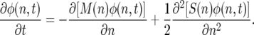(9a)

The corresponding Kolmogorov backward equation is then

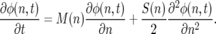(9b)

If another genotype with census number n* is introduced into the population, the corresponding equations are of course of the same form as (8) and (9), with n* in place of n. If one imposes a constraint of constant population size, such that n + n* = N (i.e., competition is such that there is a single carrying capacity for both genotypes), one can derive diffusion equations for the density function of the frequency p of the first allele, where p = n/(n + n*).

The derivation below follows the results of Demetrius and Gundlach (1999), who derived expressions of the same form for a type of demographic stochasticity induced by variances in genealogy. While the problems treated in Demetrius and Gundlach also arise from age-structured population models, the source of stochasticity is quite different; hence their variance quantities are not equivalent to those derived by Engen and colleagues.

The diffusion equations for allele (or genotype) frequency are obtained by applying the chain rule formalism for random variables proposed by Ito (see, for example, Karlin and Taylor 1975, pp. 347–348; Mikosch 1998), under the assumption of no implicit time dependence in f(n), and assuming zero covariance between n and n* (so that mixed second partials can be ignored),

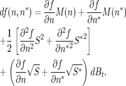By applying the Ito chain rule to the expression p(n, n*) = n(n + n*)⁻¹, the first and second partial derivatives of f with respect to n and n* can be explicitly calculated. It is assumed that a constant population size is density regulated and maintained externally by some kind of culling, so that N = n + n* for constant N. Note that it is assumed that culling occurs after reproduction, so that the subpopulations n and n* increase independently of one another prior to regulation. If reproduction were constrained to total size N prior to culling, a negative covariance between n and n* would be introduced. However, with culling following unregulated reproduction, the only covariances will be due to sampling error, which will have a random sign and therefore not contribute on average to the directions or magnitudes of the first- or second-moment terms. Note that when one genotype is rare (i.e., n* ≪ n, as in invasion analysis), these distinctions are not relevant.

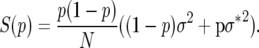
Consistent with these conditions, we have

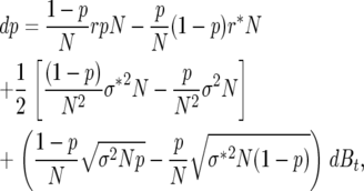(10)

where by abuse of notation, σ² = (demographic variances measured on the log scale).

The factor of the first partial term is the “drift” coefficient,

where Δr = r − r* and Δσ² = Δσ² − Δσ*².

The diffusion coefficient S(p) can be calculated directly by taking second derivatives as defined by the Ito chain rule; specifically,

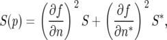which gives

The Kolmogorov backward equation for the probability density of allele frequency φ(p) with deterministic and Brownian motion coefficients corresponding to (10) is

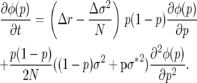(11)

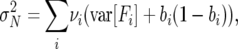
In the special case where both r and σ² are respectively equal in the two genotypes, M(p) = 0 and S(p) = p(1 − p)σ²/N, as derived in the Appendix to Engen et al. (2005b).

From Equation 11, we can obtain the effective population size of an age-structured population given demographic stochasticity,

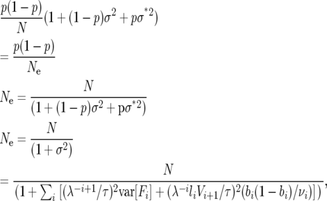which is the same as the expressions for variance effective population number calculated by Felsenstein (1971) and Hill (1972).

The above expressions for M(p) and V(p) are of course formally equivalent to Gillespie's expressions (1a) and (1b) if one substitutes demographic variance as a generalization of his variance in offspring number. As in Gillespie's equations, the coefficient of the drift term is 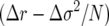rather than Δr. (Note that this argument can be readily generalized and extended to sexual diploids when fitness effects at different loci are additive or when they follow simple dominance relationships. This follows for the mean and variance in growth rate for the same reasons as for mean and variance in single-age-class fecundity analyzed by Gillespie.)

It is argued in Proulx (2000) and Shpak and Proulx (2007) that the sign of M(p) will determine whether an allele has a higher or a lower than neutral probability of fixation; i.e., when E(Δp) > 0, the probability of an allele with frequency p invading will be greater than its initial frequency, even in cases of strong selection where the diffusion approximations break down. If the contribution of demographic variance is significant, then using the expectation of the Malthusian parameter as a measure of fitness will be misleading, in that genotypes with lower values of r may actually be favored by selection as a consequence of selection acting on the second (or higher) moments.

FIXATION AND INVASION PROBABILITIES: ANALYTICAL PREDICTIONS VS. SIMULATIONS

We first consider the case of two haploid, asexual genotypes with equal average growth rate that differ in their demographic variances , . As was shown in Gillespie (1974), the diffusion estimate for fixation probability of an allele of the first type (Equation 2) in this case reduces to

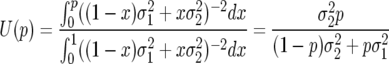(12)

so that for > , the probability of fixing the first genotype will be less than that of a neutral allele, i.e., less than its initial frequency p. This quantity is independent of population size, because while smaller N leads to a greater sample variance of growth rate, it also leads to decreased efficacy of directional selection.

For the life-history matrix

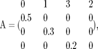the expected growth rate λ = 1.00389 (values close to unity were chosen so that population growth over multiple time steps and iterations would be minimal), and a demographic variance = 0.587288. On the log scale, we have r = 0.00388 and = 0.582747. The genotype with life-history matrix A is put into competition with genotypes with the life-history matrices

which have the same expected growth rate as A but higher respective demographic variances (6), = 1.13407, 1.73698, and 2.15947.

These rather extreme differences in fitness variance arise as a consequence of the fact that in D vs. A (for example), there is a fourfold decrease in survival probability from age class 1 to 2, compensated by a fourfold increase in age class fertilities. This leads to equal average growth rates but far greater variance in D, because a smaller fraction survive to reproductive age, while those that survive have many more offspring. It is unlikely that conspecific genotypes will have such drastic differences in their life-history parameters, so the values are chosen to illustrate the strength of selection on demographic variance rather than to model an actual scenario of intraspecific competition.

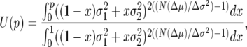
Substituting these values into (2), one can calculate the expected fixation probability of a genotype with life-history matrix A at initial frequency p in competition with B, C, or D. These predicted values are shown to correspond closely with the fixation probabilities estimated from individual-based simulations. The simulations were implemented in Mathematica (the code is available from the author upon request). For a desired total population size N, two vectors with initial age distributions were specified such that the total number of individuals in the population summed to N. In competition between genotypes with an initial frequency of 0.5, both distributions were chosen to be as close to the stable age distribution (normalized first eigenvector) as possible. In invasion analysis, a “resident” population (background of genotypes with life histories given by B, C, D, etc.) is chosen to be close to the stable age distribution while a single individual mutant with life-history matrix A is represented by one individual in the first age class.

To iterate the process, each individual in a given age class either survives or fails to do so by the next age interval with probability b_i. In the simulations, this random process is represented by selecting a value from a binomial distribution Bin(x_i, b_i), where x_i is the number of individuals of a genotype in age class i. While it is assumed for simplicity that there is no inherent variance in offspring number (so that each individual of either genotype in the ith class produces exactly m_i offspring), there is an additional parameter b₀ (set to unity in the above examples) that determines the probability of newborns surviving until the prereproductive time of census. This is simulated by choosing a random number of offspring at the census point with distribution Bin(m_ix_i, b₀), which is done for both genotypes. After the reproduction and survivorship iterations are completed, the total population size is set to N by culling numbers of individuals from each genotype and age class in proportion to their representation in the next time step.

Every cycle of survival and birth is run for as long as is necessary for one of the genotypes to become lost or fixed (i.e., the process was iterated until the frequency of one of the genotypes was zero or unity). In turn, the simulations involve several thousand trial runs, each of which is iterated until fixation or loss, so that the average number of fixation events can be calculated from a sufficiently large number of trials. It is this value, and an “empirical” estimate of fixation probability across simulations, that will be compared with the predicted value U(p).

For the simulations involving equal growth rates r, a large population size of N = 1000 was chosen to minimize the sampling error effects due to culling. Since the fixation probability is independent of population size (even though the time until fixation scales linearly with N), there is no loss of generality in using a large value of N in these examples. Table 1 shows predicted vs. observed fixation probabilities of the “A” genotype given initial frequencies p = 0.5 and p = 0.001 against B, C, and D. As can be seen, the agreement is quite close.

TABLE 1.

Expected vs. observed fixation probabilities of “A” vs. other life histories

	p = 0.5	p = 0.001
	0.661	1.94 × 10−3
	0.641	1.24 × 10−3
	0.739	2.82 × 10−3
	0.735	2.40 × 10−3
	0.787	3.70 × 10−3
	0.790	3.96 × 10−3

For competition of the A genotype against B, C, and D, the respective fixation probabilities (top values) calculated from the diffusion equation are shown in comparison with the fixation frequencies in the simulations (bottom values). Fixation probabilities in the case of effective neutrality equal the initial frequency p.

Constructing life-history matrices such that the genotype with a higher growth rate also has a higher demographic variance is straightforward, and it is fairly obvious how a trade-off leading to this scenario might arise. For instance, an organism may sacrifice its survival probability across age classes in favor of producing a higher number of offspring in a given age class, leading to a significant difference in demographic variance with or without major changes in the growth rate.

For example, contrast matrix A with

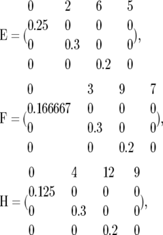which have respective expected Malthusian parameters r = 0.009558, 0.0076845, 0.00674 (all slightly larger than r_A = 0.003881) and demographic variances = 1.1482, 1.6631, 2.1705 (significantly >0.582747 for matrix A).

Equation 1a predicts that for sufficiently small population sizes, genotype A will have a higher than neutral probability of fixation. Specifically, the critical population size at which the fitness of A is equal to that of E and H is given by N , which for the three competing genotypes is 100, 284, and 555. As a consequence, it is expected to see fixation probabilities approximately equal to initial frequency p when N equals these values. For N smaller than these critical values, it is predicted that strategy A will be favored over competitors due to its lower demographic variance, in spite of having a slightly lower growth rate, while the converse should be true for sufficiently large population sizes. The discrepancy between fixation probabilities at large vs. small population sizes should of course be most pronounced when the difference in variance between strategies is greatest, as seen by comparing the genotype with Leslie matrix A to the genotype with matrix H.

Figure 1a (solid line) plots the fixation probabilities of the A genotype given an initial frequency p = 0.5 in competition against a genotype with life history E, for a range of population sizes N = 50, 100, 200, 500, and 1000. Figure 1b does the same for a single invading mutant of type A against a background of E. To correct for the fact that the initial frequency, and consequently the neutral probability of fixation, is higher in a small population (a single invading mutant has frequency 0.02 for N = 50, 0.001 for N = 1000), the fixation probabilities are multiplied by the total population sizes N. Therefore, while in Figure 1a values >0.5 indicate greater than neutral fixation probabilities, in Figure 1b values greater than unity indicate that low-variance strategy A has a higher than neutral probability of invasion. Along the same lines, Figures 2a and 3a show fixation probability of A at 50% frequency against strategies F and H, while Figures 2b and 3b show the corresponding invasion probabilities multiplied by population size N corresponding to initial frequencies of p = 1/N.

Figure 1.—

(a) Fixation probabilities of the “A” asexual, haploid genotype against the “E” genotype is plotted over a range of population sizes N, given initial frequency p = 0.5. The solid line (with points at N = 50, 100, 200, 500, and 1000) shows fixation frequencies from simulations and the dotted line the value of U(p) calculated for the same parameters. (b) Invasion probabilities (multiplied by population size N for scale) of the A genotype against a background of E genotypes are plotted over a range of population sizes N, given initial frequency p = 1/N. As in a, the solid line has points from simulations, and the dotted line is based on solutions to the Kolmogorov backward equations.

Figure 2.—

(a) The same as Figure 1a, but with competition between A and F genotypes. (b) The same as Figure 1b, but with competition between A and F genotypes.

Figure 3.—

(a) The same as Figure 1a, but with competition between A and H genotypes. (b) The same as Figure 1b, but with competition between A and H genotypes.

Superimposed against the plots of fixation frequency are solutions to Equation 2 given the same growth and variance parameters as in each simulation (shown as dotted lines in Figures 1–3). The correspondence between predicted fixation probabilities U(p) and the frequencies in the simulations is frequently not as close as those in Table 1 (where the growth rates are equal), particularly in the smaller population sizes. Furthermore, both in Table 1 and in Figures 1–3, the difference between U(p) and the simulation frequencies is more pronounced in the invasion analysis, where p = 1/N (a single invading genotype), than in competition experiments, where p = 0.5 (N/2 individuals of each genotype).

These discrepancies are a consequence of deviations from equilibrium age distributions. Working with the diffusion approximation (11) and its solutions involves reducing a description in terms of the number of individuals in each age class to a description in terms of total census number irrespective of the age class distribution. Of course, this can be done only if an equilibrium age class distribution is closely approximated. For large population sizes and large initial numbers of both genotypes, the desired distribution can readily be approximated. However, when population sizes are small or the number of any genotype is low, one or both of the age-class distributions (for the two genotypes) will be far from the equilibrium at which their growth rates and variances are estimated. This should be particularly obvious in the case of an invader, since by definition a single individual cannot be at or even closely approximate a stable age distribution! Only if the invader increases rapidly to a reasonable census number (or in special cases where most of the population consists of juveniles at equilibrium) should the univariate representation be expected to hold.

To understand how deviations from a stable age distribution can lead to misleading predictions of invasion probabilities, one must consider the population reproductive value of a genotype. For organisms with high juvenile mortality rates, the reproductive value of a newborn is almost always lower than that of the younger reproductive age classes. Therefore, the “population reproductive value” of a single juvenile will be lower than that of a population with a stable age distribution. This leads to a lower growth rate than predicted from the Leslie matrix (i.e., λ overestimates the growth rate of the rare genotype) and consequently a lower probability of invasion than is given by U(p) based on r and σ² alone.

For example, consider an A mutant juvenile invading against a background of N − 1 B individuals, where the latter are in an approximate equilibrium age distribution. The reproductive value of a juvenile A is slightly greater than unity, while the population reproductive value of B is 1.92. As a result, even though at equilibrium the expected growth rates are equal and the demographic variance of A is lower, there will be an initial bias against the invader until a critical density of later age classes is attained. This accounts in part for the invasion probabilities being in most cases lower than predicted from the diffusion approximation. Nevertheless, it should be emphasized that at least qualitatively the approximations seem to be quite robust. Even for small populations and a single invader, using growth rate and its variance in the diffusion model correctly predicts the population sizes at which the invader has a higher or a lower than neutral fixation probability.

As an aside, it was noted above that the use of growth rate and demographic variance in describing the dynamics of N(t) is an approximation that depends on the use of variance in population number as a proxy for variance in reproductive value. To determine to what extent this approximation is valid, the selection dynamics were implemented over several (t = 5, 10, etc.) generations in the presence of a single genotype, such as the one given by matrix A. For multiple trials (≥1000), the variance in N(t) was calculated. When the initial age distribution was close to ν, σ² was a good predictor for var[N(t)], within a margin of error of 10⁻³ when t was sufficiently large.

DISCUSSION

Calculating the mean and variance of growth rate allows one to describe what was a multidimensional problem (with the number of variables corresponding to d life-history stages) into a univariate dynamical system n(t). Furthermore, in the case of two genotypes, writing down coupled equations for n(t) and n*(t) and applying the appropriate transforms allows one to approximate the stochastic dynamics of p(t), the frequency of individuals of the first type in the population, in terms of the mean and variance differences in growth rate. This bivariate problem can be reduced to a univariate one as well if one posits a model of competition where genotype carrying capacities are equal and total population size is fixed.

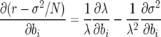
Since demographic variance can be considered an extension of Gillespie's fecundity variance to age-structured populations, it is to be expected that in a finite population, the mean growth rate λ will not generally be a sufficient predictor of whether a genotype with a given life history can invade and tend to fixation. This is due to the fact that demographic stochasticity (and growth rate variance generally) relates to population fluctuations and increased extinction probabilities (Lande et al. 2003; Engen et al. 2005a), a result that applies to multiple competing lineages as well as to the genetically monomorphic (with respect to growth rate and variance) populations studied by Lande, Engen, and colleagues. Moreover, unlike extrinsic environmental stochasticity, demographic stochasticity depends on the specific parameters of a genotype's life history and therefore contributes to the selection coefficient of the expected allele-frequency change when two genotypes are in competition. This suggests an effective selection differential measure

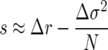and a fitness estimate for a single genotype. Since in a finite population the fixation probabilities of competing genotypes depend both on the growth rate and on demographic variance (insofar as a genotype with higher fitness has a higher than neutral probability of invasion), it is necessary to consider the effects on both first and second moments in evaluating sensitivity of fitness coefficients to changes in individual life-history parameters.

In strictly deterministic analyses of selection for life-history parameters, the sensitivity of growth rate λ with respect to age-specific parameters b_i and F_i was evaluated as the partial derivative of r or λ with respect to b_i or F_i (e.g., Hamilton 1966; Demetrius 1969). In finite populations, it may be more informative to evaluate partials of the fitness coefficients, i.e.,

(13)

For details on calculating these partial derivatives (which are rather tedious for the variance terms), the reader is referred to the appendix.

The importance of such measures hinges on the extent of the contribution of demographic variance in determining fixation probabilities. If the demographic variance itself is negligible, as would be the case in a life history where most individuals survive up to an age where most of the reproduction occurs (with little variance in offspring output per age class or individual), then a strictly deterministic approximation based on measures of mean growth rates should correctly predict the outcome of selection dynamics. When the demographic variance is not negligible (meaning that the difference in growth rate variance between two genotypes is greater than the difference in mean growth rate by a magnitude that exceeds N), the importance of the variance contribution will depend on the population size. If the population size is very large (as shown in Figures 1–3, for N = 1000), the fixation or invasion probabilities are determined almost entirely by the difference in growth rate, while for small population sizes (e.g., N = 50), the variance is the principal determinant of invasion probability.

In much of the past work on selection in age-structured populations (or any other model where an intrinsic variance in offspring number is induced), the mean growth rate has been used as a measure of fitness. This has been done on the assumption of a Poisson distribution of fecundities or on the assumption that the census population number for most model organisms tends to be large. As was argued above, fecundity variances need not be Poisson, nor are the variances induced by probabilistic models of survival.

Concerning the issue of population size, typical census numbers are in the thousands for large vertebrates and in the millions for many insects and small marine invertebrates. For such population sizes, values of Δσ²/N of comparable order to Δr are extremely unlikely, since the difference in demographic variance between genotypes of the same species tends not to be very large. In the simulation examples analyzed, extreme (and biologically unrealistic) differences in variance were induced by having 2- to 4-fold differences in survival rate compensated with equalfold differences in age class fecundities. Such matrices were chosen to illustrate the efficacy of selection against demographic variance rather than reflect biological realism.

If one assumes that the majority of mutations lead to small changes in life histories (i.e., somewhat greater degrees of iteroparity and semelparity rather than extreme changes), one should generally expect Δσ² to be of not much greater order of magnitude than Δλ. In such a case, except when population sizes are extremely small, selection on variance is not expected to be sufficiently strong to favor the genotype with lower growth rate when there are trade-offs between mean and variance in fitness or even to notably change fixation probabilities of the favored genotype from the values of U(p) predicted by standard selection and drift equations.

However, recent work (Lehmann and Balloux 2007; Shpak and Proulx 2007) suggests that for subdivided populations, census size is not an adequate predictor for the strength of selection on variance in offspring number, at least not under a regime of soft selection (sensu Wade 1985, where most of the selective culling of individuals takes place in small individual demes prior to migration, as would be the case in large social vertebrate animals and other taxa where offspring remain in local family groups until the age of sexual maturity). If the migration across demes in a metapopulation occurs among sexually mature adults, then the census size n_d of each deme (as opposed to the census size N of the metapopulation) is a better predictor for the sample variance in offspring number. This means that even for very large total N, if the individual demes are small (for instance, n_d of order 10) selection against variance in offspring number can be significant. Indeed, it was shown that this result is entirely independent of migration rate in the extreme case of “pure” soft selection.

In the case of hard selection (where migration occurs among juveniles prior to culling), it was shown that the effective population size, and therefore the outcome of selection on variance, will depend strongly on the extent of migration. Low migration rates give sample variance that scale approximately as n, approaching N for higher rates. Specifically, in the case of approximately equal allele frequencies in each deme, the deme size relevant to fecundity sample variance is

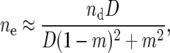(14)

which approximates n_d for low migration rates and nD = N with complete mixing.

In other words, even in seemingly large populations the contribution of intrinsic growth rate variance can be significant enough to alter the outcome of selection, when migration rates are low. Since this article shows that the demographic variance contributes to the dynamics of N(t) and p(t) in age-structured populations in the same way as offspring number (fecundity) variance in populations without age structure, the results for metapopulations should be robust for systems where both age and spatial structure are considered.

Indeed, an explicit model of age structure would allow one to investigate different degrees of hard and soft selection through the use of matrix models that combine age classes with migration between demes. By having different migration rates specific to different age classes, hard and soft selection become part of the spectrum rather than absolutes. For instance, a regime where prereproductive juveniles migrate at a relatively higher rate will tend to be more “hard” while the converse scenario more “soft.” It would be desirable to investigate how changes to life-history and migration parameters affect the outcome of selection in such a system.

The equations in Rousset and Ronce (2004) are the most general description of expected changes in allele frequency (their Equation 5) and selection coefficients (their Equations 23 and 24) in terms of the stochastic effects arising from population structure, be they spatial or with respect to age classes. The authors explicitly evaluate the selection coefficients when fecundity values are Poisson, which is not generally possible for arbitrary distributions. In principle, the equations for changes in allele frequency can be approximated as Taylor expansion in terms of the transition matrices, allowing for approximations in terms of the first two (or higher) moments. It is, however, more straightforward computationally to estimate the leading moments of the growth rate directly from the eigenvalues of the random transition matrices, as was shown in this article and in the work of Engen and colleagues. This approach gives simple closed-form expressions for the first- and second-moment terms, given arbitrary variances in each age or spatial class and the assumption of Bernoulli variances of survival rates (i.e., Equation 6 above).

The results presented in the preceding sections can be readily extended to give closed-form expressions for selection coefficients (and diffusion coefficients) in terms of the variance terms that can be calculated from derivatives of λ and the variances of matrix coefficients. The matrices themselves can represent age and stage structures in any combinations. In doing so, one would be able to reduce a multivariable system of stochastic differential or difference equations, with age classes and individual demes as state variables, to a univariate problem characterized by mean and variance of intrinsic growth rate.

APPENDIX: SENSITIVITY OF SELECTION COEFFICIENT

It is suggested that for finite populations, evaluating the partial derivatives of with respect to survival and fertility values provides a more useful measure of the sensitivity of “fitness” to changes in individual life-history parameters. By evaluation partials of s with respect to b and f, we measure the elasticity of effective fitness and estimate the strength of selection on individual b and F values when population size N is small:

(A1a)

(A1b)

Of course, the derivatives of growth rate λ are known,

The contributions from the variance terms are

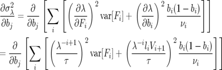(A2)

Evaluating the partial derivates, we obtain

(A3)

where the stationary distribution ν_i is

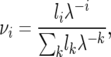so we substitute the following expression for the derivative of the stationary frequency in the second to last term of (A3) to obtain

(A4a)

if j ≥ i and

(A4b)

otherwise. The partials of λ with respect to b and F are defined above, so second partials can readily be calculated and substituted.

In the case of partials with respect to fertility parameters F, we have

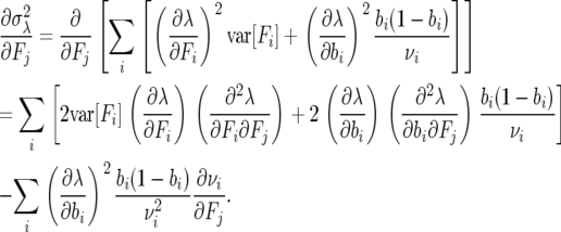(A5)

References

- Caswell, H., 2001. Matrix Population Models. Sinauer Associates, Sunderland MA.
- Charlesworth, B., 1994. Evolution in Age Structured Populations. Cambridge University Press, Cambridge, UK.
- Demetrius, L., 1969. The sensitivity of population growth rate to perturbations in the life cycle components. Math. Biosci. 4: 129–136. [Google Scholar]
- Demetrius, L., and M. Gundlach, 1999. Evolutionary dynamics in random environments, pp. 371–394 in Stochastic Dynamics, edited by H. Grauel and M. Gundlach. Springer-Verlag, New York.
- Demetrius, L., and M. Gundlach, 2000. Game theory and evolution: finite size and absolute fitness measures. Math. Biosci. 168: 9–38. [DOI] [PubMed] [Google Scholar]
- Demetrius, L., and M. Ziehe, 2007. Darwinian fitness. Theor. Popul. Biol. 72: 323–345. [DOI] [PubMed] [Google Scholar]
- Engen, S., R. Lande, B.-E. Saether and H. Weimerkirsch, 2005. a Extinction in relation to demographic and environmental stochasticity in age structured models. Math. Biosci. 195: 210–227. [DOI] [PubMed] [Google Scholar]
- Engen, S., R. Lande and B.-E. Saether, 2005. b Effective size of a fluctuating age-structured population. Genetics 170: 941–954. [DOI] [PMC free article] [PubMed] [Google Scholar]
- Engen, S., R. Lande, B.-E. Saether and M. Festa-Bianchet, 2007. Using reproductive value to estimate key parameters in density independent age structured populations. J. Theor. Biol. 244: 308–317. [DOI] [PubMed] [Google Scholar]
- Felsenstein, J., 1971. Inbreeding and variance effective numbers in populations with overlapping generations. Genetics 68: 581–597. [DOI] [PMC free article] [PubMed] [Google Scholar]
- Fisher, R. A., 1958. The Genetical Theory of Natural Selection. Oxford University Press, Oxford.
- Gillespie, J. H., 1974. Natural selection for within-generation variance in offspring number I. Genetics 76: 601–606. [DOI] [PMC free article] [PubMed] [Google Scholar]
- Gillespie, J., 1975. Natural selection for within-generation variance in offspring number II. Genetics 81: 403–413. [DOI] [PMC free article] [PubMed] [Google Scholar]
- Haldane, J. B. S., and S. D. Jayakar, 1963. Polymorphism due to selection of varying directions. J. Genet. 58: 237–242. [Google Scholar]
- Hill, W. G., 1972. Effective size of populations with overlapping generations. Theor. Popul. Biol. 3: 278–294. [DOI] [PubMed] [Google Scholar]
- Hamilton, W. D., 1966. The moulding of senescence by natural selection. J. Theor. Biol. 12: 12–45. [DOI] [PubMed] [Google Scholar]
- Karlin, S., and H. M. Taylor, 1975. A Second Course in Stochastic Processes. Academic Press, New York.
- Kimura, M., 1964. The diffusion model in population genetics. J. Appl. Probab. 1: 177–232. [Google Scholar]
- Lande, R., S. Engen and B.-E. Saether, 2003. Stochastic Population Dynamics in Ecology and Conservation. Oxford University Press, Oxford.
- Lehmann, L., and F. Balloux, 2007. Natural selection on fecundity variance in subdivided populations. Genetics 176: 361–377. [DOI] [PMC free article] [PubMed] [Google Scholar]
- Leslie, P. H., 1945. On the use of matrices in certain population models. Biometrika 33: 183–212. [DOI] [PubMed] [Google Scholar]
- Leturque, H., and F. Rousset, 2002. Convergence stability, probabilities of fixation, and the ideal free distribution in a class structured population. Theor. Popul. Biol. 62: 169–180. [DOI] [PubMed] [Google Scholar]
- Lewontin, R. C., and D. Cohen, 1969. On population growth in a randomly varying environment. Proc. Natl. Acad. Sci. USA 62: 1056–1060. [DOI] [PMC free article] [PubMed] [Google Scholar]
- Mikosch, T., 1998. Elementary Stochastic Calculus. World Scientific, Singapore.
- Proulx, S. R., 2000. The ESS under spatial variation with applications to sex allocation. Theor. Popul. Biol. 58: 33–47. [DOI] [PubMed] [Google Scholar]
- Rousset, F., and O. Ronce, 2004. Inclusive fitness for traits affecting metapopulation demography. Theor. Popul. Biol. 65: 127–141. [DOI] [PubMed] [Google Scholar]
- Seger, J., and H. J. Brockmann, 1987. What is bet-hedging?, pp. 182–211 in Oxford Surveys in Evolutionary Biology, Vol. 4, edited by P. H. Harvey and L. Partridge. Oxford University Press, Oxford.
- Shpak, M., 2005. Evolution of variance in offspring number: the effect of population size and migration. Theor. Biosci. 124: 65–85. [DOI] [PubMed] [Google Scholar]
- Shpak, M., and S. R. Proulx, 2007. The role of life cycle and migration in selection for variance in offspring number. Bull. Math. Biol. 69: 837–860. [DOI] [PubMed] [Google Scholar]
- Stearns, S. C., 2000. Daniel Bernoulli: evolution and economics under risk. J. Biosci. 25: 221–228. [DOI] [PubMed] [Google Scholar]
- Tiwari, H. K., and R. C. Elston, 1999. The approximate variance of a function of random variables. Biometric. J. 3: 351–357. [Google Scholar]
- Tuljapurkar, S. D., 1982. Population dynamics in variable environments. III. Evolutionary dynamics of r-selection. Theor. Popul. Biol. 21: 141–165. [Google Scholar]
- Tuljapurkar, S. D., and S. H. Orzack, 1980. Population dynamics in variable environments I: long run growth rates and extinction. Theor. Popul. Biol. 18: 314–342. [Google Scholar]
- Turelli, M., 1977. Random environments and stochastic calculus. Theor. Popul. Biol. 12: 140–178. [DOI] [PubMed] [Google Scholar]
- Wade, M. J., 1985. Soft selection, hard selection, kin selection, and group selection. Am. Nat. 125: 61–73. [Google Scholar]
- Wright, S., 1931. Evolution in Mendelian populations. Genetics 16: 97–159. [DOI] [PMC free article] [PubMed] [Google Scholar]