The Evolution of Two Mutations During Clonal Expansion

Abstract

Knudson's two-hit hypothesis proposes that two genetic changes in the RB1 gene are the rate-limiting steps of retinoblastoma. In the inherited form of this childhood eye cancer, only one mutation emerges during somatic cell divisions while in sporadic cases, both alleles of RB1 are inactivated in the growing retina. Sporadic retinoblastoma serves as an example of a situation in which two mutations are accumulated during clonal expansion of a cell population. Other examples include evolution of resistance against anticancer combination therapy and inactivation of both alleles of a metastasis-suppressor gene during tumor growth. In this article, we consider an exponentially growing population of cells that must evolve two mutations to (i) evade treatment, (ii) make a step toward (invasive) cancer, or (iii) display a disease phenotype. We calculate the probability that the population has evolved both mutations before it reaches a certain size. This probability depends on the rates at which the two mutations arise; the growth and death rates of cells carrying none, one, or both mutations; and the size the cell population reaches. Further, we develop a formula for the expected number of cells carrying both mutations when the final population size is reached. Our theory establishes an understanding of the dynamics of two mutations during clonal expansion.

THE concept of a tumor-suppressor gene originated from a statistical analysis of retinoblastoma incidence (Knudson 1971). This and later work (Moolgavkar and Knudson 1981; Friend et al. 1986; Vogelstein and Kinzler 2002) led to Knudson's two-hit hypothesis suggesting that retinoblastoma develops due to the inactivation of both alleles of the RB1 gene. The inherited form of the disease results from a germ-line mutation in one allele followed by inactivation of the second allele during somatic cell divisions. In sporadic retinoblastoma, both mutations arise during retina development. An understanding of the tumorigenesis of sporadic retinoblastoma requires the study of the dynamics of RB1 mutations during the growth of the retina. What is the chance that both alleles have been inactivated before the retina reaches its final size? How does this probability scale with mutation rates and cell turnover? And how large is a retinoblastoma tumor expected to be?

Tumor metastasis is a significant contributor to death in cancer patients. Metastases arise when cancer cells leave the primary tumor site and form new colonies elsewhere (Chambers et al. 2002). Metastasis formation can be driven by genetic alteration of many genes, including activation of oncogenes like RAS and MYC (Pozzatti et al. 1986; Wyllie et al. 1987) and inactivation of metastasis-suppressor genes such as NM23 (Steeg et al. 1988; Steeg 2004). Metastasis suppressors maintain the normal, noninvasive state of cells, and their inactivation promotes metastasis formation. It is clinically relevant to know whether a growing tumor has already inactivated a metastasis suppressor when it is diagnosed. What is the probability that a clonally expanding tumor cell population has accumulated two mutations in a metastasis suppressor gene before detection? How many metastasis-enabled cells does such a tumor contain?

Acquired drug resistance is a threat for the successful treatment of cancer (Gottesman 2002). Depending on therapy, the type of cancer, and its stage, one or several (epi)genetic alterations are necessary to confer resistance to treatment. Some mechanisms of resistance require two genetic alterations—either because of haplosufficiency of a gene such that one recessive mutation cannot confer resistance or because of the use of combination therapy that targets two different positions in the cancer genome. Examples of the former are inactivation of p53, ATM, and RB1 (Lowe et al. 1994; Volm and Stammler 1996; Westphal et al. 1997). An example of the latter is emerging resistance of chronic myeloid leukemia cells against combination therapy with imatinib (Gleevec, STI571) and dasatinib (BMS-35482) (Shah et al. 2004, 2007). Although both agents target the BCR–ABL kinase domain, the spectra of mutations conferring resistance to these drugs do not overlap—apart from one point mutation, which causes resistance to both (Tokarski et al. 2006). It is important to know whether patients already have resistant cells at diagnosis because this determines treatment strategies.

These examples lead to the following two questions: (i) What is the probability that an exponentially expanding cell population evolves two mutations before reaching a certain size?, and (ii) What is the expected number of such cells at that time? In this article, we study the dynamics of two mutations emerging in a growing population of cells. Earlier, we analyzed the dynamics of one mutation arising during clonal expansion (Iwasa et al. 2006) as well as the dynamics of two mutations emerging in a population of constant size (Michor and Iwasa 2006). Our studies are akin to Luria and Delbrück's investigation of the mutations conferring bacterial resistance to phages (Luria and Delbrück 1943). The distribution of mutants in an exponentially growing population is known as the Luria–Delbrück distribution and has been studied extensively (Tlsty et al. 1989; Zheng 1999; Frank 2003). These studies are based on pure birth processes and neglect the possibility of cell death. In most situations in cancer, disease, and development, however, cell death does occur. Therefore, we introduce a birth-and-death model and calculate the probability that both mutations have arisen once the population reaches its final size, as well as the expected number of such cells at that time. This work is part of a growing effort to study cancer with mathematical techniques (Nordling 1953; Armitage and Doll 1954, 1957; Fisher 1959; Goldie and Coldman 1979; Moolgavkar and Knudson 1981; Luebeck and Moolgavkar 2002; Michor et al. 2004, 2005; Wodarz and Komarova 2005; Iwasa et al. 2006; Michor and Iwasa 2006).

THE MODEL

Consider an exponentially growing population of cells starting from a single cell that is wild type at both genomic positions of interest. Cells wild type at both positions are called type-0 cells, and they give rise to cells harboring a mutation at one position with probability u₁ per cell division. Cells carrying one mutation are called type-1 cells, and they produce cells harboring mutations at both positions with probability u₂ per cell division. Such cells are called type-2 cells (Figure 1). The term “mutation” is collectively used to describe point mutations, insertions, deletions, inversions, translocations, loss of heterozygosity, and other genetic aberrations that can occur during one cell division. We focus on only two genomic positions and consider the mutational background as constant across cell types.

Figure 1.—

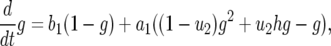
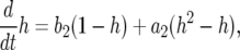
Evolution of two mutations. A cell wild type at both positions is called a type-0 cell; it divides at rate r and dies at rate d. A cell carrying one mutation is called a type-1 cell. It arises by mutation of a type-0 cell at rate u₁ per cell division; it divides at rate a₁ and dies at rate b₁. A cell carrying two mutations is called a type-2 cell. It arises by mutation of a type-1 cell at rate u₂ per cell division; it divides at rate a₂ and dies at rate b₂.

The cell population follows a continuous-time branching process. Denote the growth rates of type-0, type-1, and type-2 cells by r, a₁, and a₂ and their death rates by d, b₁, and b₂. If a₁>r, then the first mutation is advantageous and increases the fitness of the cell; if a₁ = r, then the first mutation is neutral and does not change the fitness; and if , then the mutation is disadvantageous and decreases the fitness of the cell. Similar comparisons apply to the fitness of type-2 cells. Detection occurs once the total population size—the sum of the number of type-0, type-1, and type-2 cells—reaches size M.

Computer simulations:

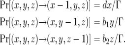
We perform exact computer simulations of the stochastic process. There are three types of cells: type-0, type-1, and type-2 cells. Their respective numbers are denoted by x, y, and z. A change in x, y, and z occurs by cell division (possibly with mutation) or by cell death. Initially, there is one type-0 cell, x = 1, and no mutant cell, y = z = 0.

The stochastic simulation is performed by first determining which of the possible events (production or death of a type-0, a type-1, or a type-2 cell) is likely to occur first; the chance of each event to be first is proportional to its rate normalized by the sum of the rates of all possible events. Let us denote this sum by R. Then the timing of the first event is given by a negative exponential distribution with mean 1/R. The process is continued either until all cells go extinct, 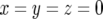, or until the total cell number reaches the final size, 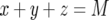. The transition probabilities between states are determined as follows. The number of type-0 cells increases if a type-0 cell divides without mutating. Hence the probability that the number of type-0 cells increases by one is given by

(1a)

where . The number of type-1 cells increases by mutation of a type-0 cell or by division of a type-1 cell without mutation. The probability that the number of type-1 cells increases by one is given by

(1b)

The number of type-2 cells increases by mutation of a type-1 cell or by division of a type-2 cell. We neglect the possibility of two mutations emerging during one cell division because this probability is sufficiently small. Hence the probability that the number of type-2 cells increases by one is given by

(1c)

The probabilities that the numbers of type-0, type-1, and type-2 cells decrease by one are given by

(1d)

For each parameter set, we perform many independent runs of the stochastic process to account for random fluctuations and count the fraction of runs that reach the final size, M, and have produced at least one type-2 cell. We also record the number of type-2 cells in those runs.

The probability of two mutations:

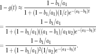
Let us now derive an analytic expression for the probability that an exponentially growing population, starting from one type-0 cell, has produced at least one type-2 cell until the total population size reaches M. For simplicity, we assume that the death rates are constant across cell types, .

Branching-process formula:

Let us first use a multistate branching process to calculate the probability of two mutations. This calculation is based on the assumption that the number of type-1 and type-2 cells is much smaller than the number of type-0 cells; hence we adopt the approximation that the final population size is reached once the number of type-0 cells becomes M. This approach represents an extension of earlier work (Iwasa et al. 2006). The calculation is subdivided into two parts: (i) considering the number of type-1 cells produced from the exponentially expanding population of type-0 cells and (ii) studying the behavior of a cell lineage originating from a single type-1 cell. The generating function of the total number of type-2 cells is given by

(2)

Here is the generating function of a lineage starting from a single type-1 cell, and R_x is the expected number of newly created type-1 cells when there are x type-0 cells; it is given by 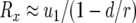(Iwasa et al. 2006).

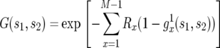
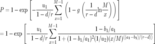
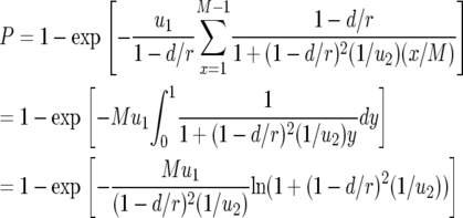
The generating function, Equation 2, can be used to calculate important quantities. The probability that there are no type-2 cells—irrespective of the number of type-1 cells—once the total population size reaches M is given by

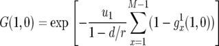(3)

Hence the probability that there is at least one type-2 cell when the population reaches its final size is given by

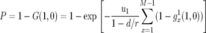(4)

appendix a contains the derivation of and the derivation of the probability of two mutations in the neutral case, , which is given by

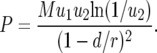(5)

Let us now compare Equation 5 with the direct computer simulation. Figure 2 shows that the prediction of Equation 5 (solid curve) is a slight overestimation of the probability of two mutations represented by the results of the direct computer simulation (open circles). The formula for deleterious mutations is more accurate, while the formula for advantageous mutations gives a significant overestimation (data not shown). The deviation stems from the assumption of the analytic solution that the final population size is reached once there are M type-0 cells, rather than once the sum of type-0, type-1, and type-2 cells reaches M. This assumption leads to accurate predictions of the probability of having type-1 cells (Iwasa et al. 2006), but to an overestimation of the probability of having type-2 cells—particularly if type-1 cells have a fitness advantage and can reach significant fractions of the final population size. Therefore, we consider a different analytic approach in the following.

Figure 2.—

The probability of two neutral mutations ( ). The probability of having produced at least one type-2 cell once the population reaches size M in dependence of the mutation rate of type-0 cells, u₁ (a), the mutation rate of type-1 cells, u₂ (b), the growth rate of all cell types, (c), and the final population size, M (d), is shown. The solid curve shows the prediction of Equation 5, the open circles show the results of the exact computer simulation, and the dots show the prediction of the alternative formula, Equation 9. 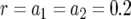Parameter values are and (a) , , and ; (b) , , and ; (c) , , and ; and (d) , , and .

Alternative formula:

Let us consider the two steps required for the emergence of type-2 cells: (i) production of a type-1 cell and the survival of its lineage and (ii) production of a type-2 cell and its persistence. Denote by the probability that the first step occurs when there are x type-0 cells. With 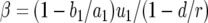, we have

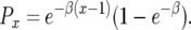(6)

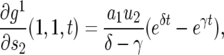
See appendix b for the derivation of P_x. The population of cells now contains x type-0 cells and one (eventually successful) type-1 cell. It is in this lineage that a surviving type-2 cell emerges. A type-2 cell may arise by mutation during each division of a type-1 cell. The expected number of mutational events is proportional to the total number of cell divisions the type-1 cell lineage experiences until the final population size is reached. The total number of type-1 cell divisions is on average , where y is the abundance of type-1 cells at detection. Therefore the probability, Q_x, of producing a type-2 cell in a type-1 cell lineage is given by

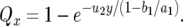(7)

Here , and is the time between the emergence of a type-1 cell from x type-0 cells and when the total number of type-0 and type-1 cells reaches M. See appendix b for the formula of and the derivation of Q_x.

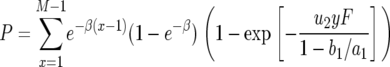
With these results, the probability that there is at least one type-2 cell when the total population size reaches M is given by

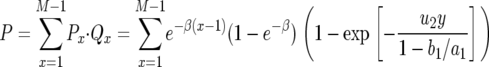(8)

This expression holds if the death rates of type-2 cells can be neglected as compared to the growth rates. If the mortality of type-2 cells cannot be neglected, there is an additional factor in the equation (see appendix b). In the neutral case ( ), we can simplify Equation 8 as

(9)

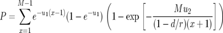
Let us now compare Equation 8 with the stochastic computer simulation. Figure 3 shows the agreement between the predictions of the formula (dots) and the results of the simulation (open circles). The model includes seven parameters: the population size at detection (M), the probability of mutating either genomic position per cell division (u₁ and u₂), the growth rate of type-0, type-1, and type-2 cells (r, a₁, and a₂), and the death rate (d). If the four rates r, a₁, a₂, and d are multiplied by the same factor, then the whole process proceeds faster but the probability P remains constant. Hence P is determined by the three ratios a₁/r, a₂/r, and d/r rather than by the four rates independently. In the following analysis of the parameter dependence, we examine the case with r = 1 (without loss of generality) and consider the formula in which a₁, a₂, and d are replaced by a₁/r, a₂/r, and d/r, respectively:

1. Probability of mutating the first position, u₁: As shown in Figure 3a, the probability of two mutations, P, increases with u₁. High values of u₁ increase the risk of producing a type-1 cell lineage that can eventually give rise to type-2 cells.

2. Probability of mutating the second position, u₂: As shown in Figure 3b, the probability of two mutations, P, increases with u₂. High values of u₂ increase the chance that type-2 cells emerge.

3. Relative growth rate of type-1 cells, a₁/r: As shown in Figure 3, a and b, the probability of two mutations, P, increases with a₁/r: A larger growth rate of type-1 cells relative to that of type-0 cells enhances the chance of two mutations because type-1 cells can reach higher frequencies.

4. Relative growth rate of type-2 cells, a₂/r: The probability of two mutations, P, is almost independent of the relative growth rate of type-2 cells, a₂/r (data not shown). This effect emerges because here we focus on the existence of type-2 cells rather than on their abundance. The growth rate of type-2 cells does not significantly affect the probability of successfully establishing a lineage from a single cell; as long as the growth rate is clearly greater than the death rate, the newly produced mutant will almost certainly survive. Once a lineage of type-2 cells has emerged, the growth rate of type-2 cells has no effect on the chance of their existence once the population reaches its final size—it does, however, have an important effect on their abundance, as discussed later.

5. Relative death rate, d/r: As shown in Figure 3c, the probability of two mutations, P, increases with d/r. A large death rate prolongs the time it takes until the total population reaches size M. It increases the number of cell divisions and therefore enhances the chance of accumulating mutations.

6. Final population size, M: As shown in Figure 3c, the probability of two mutations, P, increases almost linearly with M. This effect emphasizes the importance of detecting a growing population of cancer cells as early as possible to reduce the risk of having evolved two mutations.

Figure 3.—

The probability of two mutations. The probability of having produced at least one cell mutated in both positions when the cell population reaches size M in dependence of the growth rate of cells mutated in one position, a₁ (a and b), and the final population size, M (c), is shown. Equation 8 is shown as dots and the direct computer simulation (system 1) as circles. Parameter values are (a) , (line 1), and (line 2); (b) , (line 1), and (line 2); and (c) , , , , (line 1), and (line 2).

We performed a regression analysis of Equation 8 to analyze the sensitivity of the probability P with respect to the parameters. Using many different parameter sets, we obtained the following regression formula:

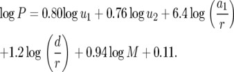(10)

The ratio of the results from the regression formula to that from Equation 8 ranges from −0.3 to 0.3 in logarithmic units. The formula indicates that every parameter except a₂/r (the relative growth rate of type-2 cells) affects the probability P. Note that the coefficient for is the largest among all terms, implying that an increase in the growth rate of type-1 cells most effectively enhances the risk of two mutations. Note also that the coefficient for is positive, signifying that a higher death rate increases the risk. A larger death rate necessitates a larger number of cell divisions to reach a certain population size, and hence the chance of mutations increases. Finally, Equation 10 indicates that P decreases with the growth rate of type-0 cells, r. Hence a large growth rate of type-0 cells reduces the risk of two mutations—fast-growing tumors are more likely to be sensitive to treatment than slowly growing ones.

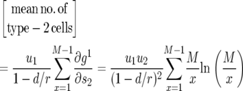
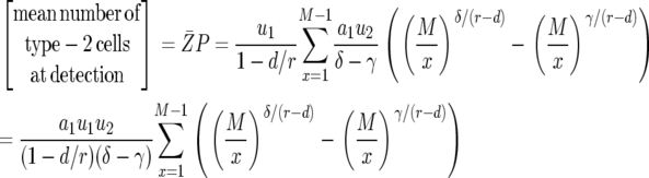
The expected number of cells with two mutations:

Let us now calculate the expected mean number of type-2 cells once the population reaches its final size.

Branching-process formula:

The mean number of type-2 cells in a lineage starting from a single type-1 cell is calculated from Equations 2 and A1 by taking the derivative with respect to s₂ and setting . According to the calculation in appendix c, we have

(11)

with and . In the neutral case, and , the difference between and becomes very small, , and we can approximate Equation 11 by

(12)

The duration between the time when there are x type-0 cells and the time when the final population size is reached is given by (Iwasa et al. 2006). Then we have

(13)

The expected number of type-2 cells once the population reaches its final size is given by the derivative of Equation 2 with respect to s₂ evaluated at and 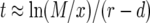, which is

(14)

The mean number of type-2 cells among those with at least one type-2 cell is given by Equation 14 divided by the probability to have any type-2 cells, P:

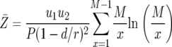(15)

It can be seen from Equation 14 that the expected number of type-2 cells decreases with the ratio r/d. When r is close to d (and greater than one), the number of type-2 cells is very large. When the ratio r/d becomes very large, the cell number converges to an asymptote independent of r and d. A formula for the expected number of cells in the nonneutral case can be derived similarly (see appendix c).

A comparison between the formula and the direct computer simulation shows that the formula is accurate for neutral mutations (Table 1), but tends to overestimate the number of type-2 cells when the mutations are advantageous (data not shown) for the same reason as above. Therefore, we again consider an alternative approach.

TABLE 1.

Comparison of Equation 15 with the computer simulation in the neutral case

		Parameter enhanced by 50%
	Standarda			M	d/r
Computer simulation	15.5	17.6	18.0	19.0	31.4
Equation 15	15.4	16.6	17.3	17.5	25.7

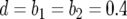
^aThe standard parameter set is given by , , , and . Each specified parameter is enhanced by 50% while all the other parameters remain constant. Equation 15 gives good predictions of the expected number of type-2 cells in the neutral case.

Alternative formula:

Note that we have already derived the probability of type-2 cells (P) and the number of type-1 cells (y) once the final population size is reached, as well as the length of time between the emergence of type-1 cells and when the sum of type-0 and type-1 cells reaches M ( ). Denote by Z the number of type-2 cells once the final size is reached. If we adopt the assumption that type-2 cells experience deterministic growth, then the number Z is determined by the time of emergence of the first type-2 cell. Hence the probability that the number of type-2 cells, Z, is between z₁ and z₂ equals the probability that the first type-2 cells emerges between times t₁ and t₂ (for a schematic explanation, see Figure 4). Then we obtain a formula for 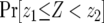and can further derive the mean number of type-2 cells, (see appendix d).

Figure 4.—

Schematic representation of how to calculate the expected number of type-2 cells. The horizontal axis shows the time since initiating growth with one type-0 cell. The vertical axis shows the logarithmic number of the three cell types. Type-0, type-1, and type-2 cells undergo exponential growth at rates , , and , respectively, which appear as three lines with different slopes. A mutation is created at a Poisson rate, as indicated by the two arrows. It takes time units for a lineage of type-1 cells to reach y and time units for a lineage of type-2 cells to reach Z.

The probability distribution of the number of type-2 cells is shown in Figure 5. The prediction of Equation D4 (red line) is in good agreement with the results of the computer simulation (black dots, see appendix d for details). Table 2 shows the parameter dependence of the expected number of type-2 cells by comparing the standard parameter set with sets in which one of the six parameters u₁, u₂, M, a₁/r, a₂/r, and d/r is enhanced by 50%. For each parameter set, we performed >100,000 runs and calculated the conditional mean number of type-2 cells. This number increases with the enhancement of each parameter except the growth rate of type-1 cells, a₁/r; interestingly, the latter enhancement reduces the cell number while it increases the probability of having at least one type-2 cell. This effect emerges because the total population reaches size M before type-2 cells gain a significant frequency if the growth rate of type-1 cells is large. Therefore, the consequence of a large growth rate of type-1 cells is a high probability of producing type-2 cells, but a small number of such cells that may be difficult to observe. In contrast, a higher relative death rate ( d/r) increases the number of type-2 cells because in that case, it takes longer for the total population to reach M and type-2 cells are likely to increase during that time. The most effective parameter to influence the expected number of type-2 cells is their growth rate; this parameter, however, does not affect the probability of having type-2 cells.

Figure 5.—

The probability distribution of the number of type-2 cells. We show the probability distribution of type-2 cells for different values of the growth rate of type-1 cells, a₁. Red lines indicate the predictions of Equation D4 and black dots show the results of the stochastic computer simulation. The horizontal axis shows the number of type-2 cells, Z, and the vertical axis is , the probability that Z is equal to z. Parameter values are , , , , , and and (a) , (b) , and (c) .

TABLE 2.

The mean number of type-2 cells

		Parameter enhanced by 50%
	Standarda						d/r
Mean no. of type-2 cells	82.0	90.7	112.5	131.1	41.9	1675.0	101.5

^aThe standard parameter set is given by , , , , , and . Each specified parameter is enhanced by 50% while all the other parameters remain constant. Enhancement of the relative growth rate of type-1 cells reduces the mean number of type-2 cells, but enhancement of each of the other parameters increases the mean number once the final population size is reached.

DISCUSSION

In this article, we study the dynamics of two mutations arising in an exponentially growing population of cells. We calculate the probability of having produced at least one cell with two mutations once the population reaches a certain size, as well as the distribution of the number of such cells at that time. These results are important in many medical scenarios. For instance, chronic myeloid leukemia (CML) patients treated with imatinib and dasatinib readily evolve several resistance mutations (Shah et al. 2007). A clinically relevant question is whether such compound resistance mutations are preexisting to diagnosis of CML, because this influences treatment choices. Our mathematical framework allows us to calculate the probability that a patient harbors an imatinib- and a dasatinib-resistant mutation, as well as the number of such cells, at the time of diagnosis (Table 3). We find that the chance is nonnegligible that both mutations emerge before diagnosis.

TABLE 3.

The probability of a compound-resistant mutation

	Mutation rates
Cell turnover	u1 = 50 × 10−8, u2 = 10 × 10−8	u1 = 50 × 10−7, u2 = 10 × 10−7	= 50 × 10−6, =10 × 10−6
d = 0.003	P = 1.3 × 10−6	P = 0.0001	P = 0.0091
r = 0.008	= 44.6	= 46.5	= 60.7
a1 = 0.010
a2 = 0.012
d = 1.003	P = 1.6 × 10−6	P = 0.0002	P = 0.0112
r = 1.008	= 44.7	= 46.7	= 61.3
a1 = 1.010
a2 = 1.012
d = 1.003	P = 6.9 × 10−5	P = 0.0063	P = 0.3008
r = 1.008	= 774.5	= 816.4	= 1312.6
a1 = 1.016
a2 = 1.032
d = 1.003	P = 0.0093	P = 0.2183	P = 0.9395
r = 1.008	= 8068.3	= 8326.7	= 9487.8
a1 = 1.080
a2 = 1.800

We show the probability P that a patient harbors an imatinib- and a dasatinib-resistant mutation when diagnosed with chronic myeloid leukemia (CML) and the expected number of such cells, , at diagnosis. The net growth rate of leukemic stem cells before diagnosis is about (r − d) = 0.005/day (Michor et al. 2005), and we provide several examples of growth and death rates. At diagnosis, there are ∼M = 250,000 leukemic stem cells (Holyoake et al. 2002).

We have presented two approaches to calculating the probability of having two mutations once the total population reaches a certain size. One approach is based on a multistate branching process. This methodology can be used to derive an analytic expression for the probability of two mutations as well as the probability distribution of cells. It is very accurate for mutations that confer a fitness disadvantage to the cell or that are neutral as compared to wild-type cells. The second approach requires some numerical calculation, but is very accurate when the mutations confer a fitness advantage to the cell and when they are neutral. To provide mathematical solutions for all scenarios, we present both approaches in this article.

An investigation of the probability of two mutations informs us about the importance of particular parameter values in the process. The relative growth rate of cells harboring one mutation (type-1 cells) is decisive for the probability of eventually producing two mutations. This feature suggests experimentally determining the growth rates of type-0 cells (which carry no mutation) and type-1 cells to predict the presence of two mutations. If the ratio of the growth rate of type-1 cells to the growth rate of type-0 cells is high, then the probability of two mutations is large. Therefore, the abundance of type-1 cells is a good proxy for the presence of type-2 cells (which harbor both mutations). Furthermore, large death rates increase the chance of accumulating mutations because the risk increases with the number of cell divisions generating the cell population; a population of a particular size will contain many more mutants if the cell turnover is large. Hence tumors with high apoptosis rates are at particular risk of containing resistant cells. Last, the mutation rates themselves increase the probability of mutations, and hence therapies that induce genetic instabilities or work by damaging DNA enhance the chance of treatment failure.

We have also investigated the probability distribution of the number of type-2 cells. The parameter that most effectively influences the number of those cells is their relative growth rate, which in turn does not affect the probability of having any type-2 cells. Interestingly, high relative growth rates of type-1 cells increase the probability that type-2 cells exist, but reduce their number. On the basis of our theory, the worst case is represented by a large relative growth rate of type-1 cells (which increases the probability that a type-2 cell emerges) and an even larger relative growth rate of type-2 cells (which ensures that such cells can grow). A situation requiring particular attention occurs when the growth rate of type-1 cells is larger than the growth rates of both type-0 and type-2 cells, because then a small number of type-2 cells exist with high probability, but those cells will be difficult to detect.

So far, we have assumed that the mutation rates are constant throughout tumor growth. However, genomic instabilities lead to increasing rates of genetic changes and are a frequent property of tumors (Lengauer et al. 1998). Figure 6 demonstrates how increasing mutation rates influence the evolutionary dynamics of two mutations. As compared to constant mutation rates, continuously increasing rates lead to elevated probabilities of harboring two mutations. However, the mean number of cells with two mutations decreases in such scenarios (Table 4). This effect emerges because large mutation rates enhance the production of cells carrying two mutations, particularly when the population size is large, and therefore lead to more patients harboring fewer such cells. Our finding emphasizes the danger of genetically unstable lesions for treatment outcomes, as well as the necessity to use anticancer drugs that do not increase genomic mutation rates.

Figure 6.—

The effect of increasing mutation rates on the probability of two mutations. The probability of having produced at least one type-2 cell once the population reaches size M in dependence of the final population size (M) is shown. We examine situations in which the mutation rates, u₁ and u₂, each increase by each 1000 times type-0 cells and type-1 cells divide, respectively. We show that the probability of two mutations increases with the value of . Line 4 represents the same results as line 2 in Figure 3c. The parameter values are , , , , , and and (line 1), (line 2), (line 3), and (line 4).

TABLE 4.

The effect of increasing mutation rates on the mean number of type-2 cells

Mean no. of type-2 cells	70.9	28.5	11.3	8.3

The mean number of cells carrying two mutations for different enhancement factors of the mutation rates, , is shown. The mean number decreases as increases. Parameter values are , , , , , , and M = 500,000. We performed >10,000 runs in which at least one type-2 cell is present when M is reached.

This article increases our knowledge of the evolutionary dynamics of an exponentially expanding population. An important goal of the field is to generalize our algorithm to arbitrary mutation–selection networks such that the probability of having n mutations (emerging in a particular order) in a growing population can be calculated and the expected number of cells harboring these mutations can be predicted. Further, the calculation may be adapted to describe situations in which more than one offspring arises per division event; such scenarios arise in infectious diseases such as human immunodeficiency virus (HIV). Haeno and Iwasa (2007) consider the risk of drug resistance of an exponentially growing virus, assuming that infected cells give rise to a random number of virus particles per time interval. They derive a formula for the probability of one mutation at detection and show its implications for HIV primary infection. Our formulation of the probability of two mutations with regard to (cancer) cell division inspires an approach to calculate the probability of two mutations with regard to virus proliferation.

APPENDIX A: DERIVATION OF THE BRANCHING-PROCESS FORMULA FOR THE PROBABILITY OF TWO MUTATIONS

Denote by the generating function for a lineage starting from a single type-1 cell and by the generating function for a lineage starting from a single type-2 cell. Their equations satisfy the recursive formulas

(A1a)

(A1b)

with the initial conditions and .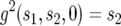

Let be the probability that there is one type-1 cell and no type-2 cell at time t. Similarly, let 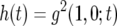be the probability that there is no type-1 cell and one type-2 cell at time t. Then system (A1) becomes

(A2a)

(A2b)

with the initial conditions and . As Equation A2a does not have an explicit solution, we adopt the following approximation. Suppose we have a solution of for . We convert this solution to a function of x by assuming deterministic exponential growth of type-0 cells, . Hence we have

(A3)

The solution of Equation A2b is given by

(A4)

However, as shown in the following, h(t) does not contribute to the result of P. Equation A2a is rewritten as

(A5)

with . If we neglect the second term, which is of the order of u₂, this equation is similar to a logistic equation and has two equilibria: and . Starting from , the solution stays in the unstable equilibrium . Now note that the second term of Equation A5 is negative because g(0) = 1 and h(0) = 0. For small t, this term is approximately and pushes the system away from the unstable equilibrium . Once the system is perturbed, it converges to the other equilibrium at following the dynamics determined by the first term. The second term is therefore important only for small t, and we can approximate Equation A5 as

(A6)

When t = 0, Equation A6 equals Equation A5. With and , we have

(A7)

By noting that is a small quantity and is a very large quantity, Equation A7 becomes

(A8)

Using , we have

(A9)

In the neutral case, , we can further simplify the formula as follows:

(A10)

We can further simplify the formula to obtain Equation 5 in the text.

APPENDIX B: DERIVATION OF THE ALTERNATIVE FORMULA FOR THE PROBABILITY OF TWO MUTATIONS

Let P_x be the probability that the first successful lineage of type-1 cells arises when there are x type-0 cells. This probability can be written as the product of the probability that no successful type-1 cell lineage arises when there are 1, 2, 3, … , x − 1 type-0 cells and the probability that a successful type-1 cell lineage is created when there are exactly x type-0 cells. We assume that the number of mutants created when there are x type-0 cells follows a Poisson distribution with mean R_x (Iwasa et al. 2006). A fraction of these new mutations survives the initial stochastic fluctuations and results in exponentially growing lineages. This fraction is given by , the nonextinction probability. Hence we have 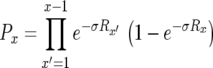. With 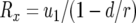(Iwasa et al. 2006) and , we obtain Equation 6 in the text.

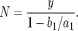
Next we consider the probability that a type-2 cell is created within a lineage that starts from one type-1 cell. Let y be the number of type-1 cells present when the total cell population reaches size M, and let N be the mean number of type-1 cell division events that occur while type-1 cells increase from 1 cell to y cells. The per capita rate of increase in their number is given by , and the per capita rate of cell division is given by a₁. Hence we have 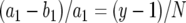. With y ≫ 1, this expression becomes

(B1)

During each cell division, a type-2 cell emerges with probability u₂. Hence the probability that at least one type-2 cell arises in such a lineage is given by with . Note that is the length of time between the emergence of a successful type-1 cell and when the total number of type-0 and type-1 cells reaches M. If , we have

(B2)

Here is the number of type-0 cells, is the number of type-1 cells, and their sum equals M. Equation B2 is a transcendental equation and has to be solved numerically to obtain .

With these results, the probability that there is at least one type-2 cell when the total population size reaches M is given by Equation 8 in the text. This expression holds if the death rates of type-2 cells can be neglected as compared to their growth rates. If the mortality of type-2 cells cannot be neglected, we replace Q_x by the formula in Iwasa et al. (2006) and obtain

(B3)

Here 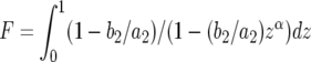and .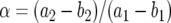

APPENDIX C: BRANCHING-PROCESS FORMULA FOR THE EXPECTED NUMBER OF TYPE-2 CELLS—DELETERIOUS AND ADVANTAGEOUS CASES

The expected number of type-2 cells is obtained by taking the derivative of the generating function, Equation 2, with respect to s₂ and evaluating it at . We first take the derivative of the differential equations for the generating functions, Equation A1, with respect to s₂. Then we obtain a pair of linear equations, which leads to the solution given by Equation 11 in the text.

After having discussed the neutral case in the main text, we focus here on nonneutral cases. From Equation 11 and with , we have

(C1)

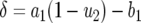with and . Hence the expected number of type-2 cells once the total population reaches size M is

(C2)

The mean number of type-2 cells among those with at least one type-2 cell is

(C3)

APPENDIX D: ALTERNATIVE FORMULA FOR THE EXPECTED NUMBER OF TYPE-2 CELLS

Let us consider the number of type-2 cells once the population reaches its final size by approximating their growth with deterministic dynamics (see Figure 4 for a schematic explanation). Note that we have already derived the probability that at least one type-2 cell exists, P, the number of type-1 cells, y, and the length of time between the emergence of the first type-1 cell and when the total number of type-0 and type-1 cells reaches M, . Now we consider the probability that the number of type-2 cells is less than a given value once the total population size reaches M. Let Z be the number of type-2 cells, and let be the time it takes from the appearance of the first type-2 cell until the final size is reached (Figure 4). From the assumption that type-2 cells grow exponentially, we have 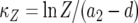. Then the probability that the number of type-2 cells, Z, is less than with is given by

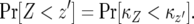(D1)

Note that we have already calculated , and this expression approximately represents the length of time between the emergence of a type-1 cell from x type-0 cells and when the final population size is reached. Then the probability that the number of type-2 cells, Z, is less than is expressed as the probability that no type-2 cell lineage emerges during and that a type-2 cell lineage appears thereafter. Let S be the probability that a type-2 cell lineage appears during . The probability, Q_x, that a type-2 cell lineage appears during has already been derived. Therefore, the probability that no type-2 cell lineage emerges during and that a type-2 cell lineage appears thereafter is expressed as . Considering that the population starts from one type-0 cell and excluding the cases in which no type-2 cells emerge, we have

(D2)

Since we sum all cases from , the cases where must be considered. When , the number of the type-2 cells is always less than . Hence S is given by

(D3)

Note that the probability is conditional to the existence of several type-2 cells.

Finally, let us discuss the probability distribution of the number of type-2 cells. According to Equation D2, the probability that the number of type-2 cells is between z₁ and z₂ with 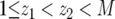is given by

(D4)

From using Equation D4, we can derive the expected number of type-2 cells numerically as

(D5)

In Figure 5, the dots represent the results of the computer simulation, system 1. We record the number of type-2 cells once the total population size (including type-2 cells) reaches M and calculate the distribution frequency. We perform >40,000 runs of this process to generate each figure.

References

- Armitage, P., and R. Doll, 1954. The age distribution of cancer and a multi-stage theory of carcinogenesis. Br. J. Cancer 8: 1–12. [DOI] [PMC free article] [PubMed] [Google Scholar]
- Armitage, P., and R. Doll, 1957. A two-stage theory of carcinogenesis in relation to the age distribution of human cancer. Br. J. Cancer 11: 161–169. [DOI] [PMC free article] [PubMed] [Google Scholar]
- Chambers, A., A. Groom and I. MacDonald, 2002. Dissemination and growth of cancer cells in metastatic sites. Nat. Rev. Cancer 2: 563–572. [DOI] [PubMed] [Google Scholar]
- Fisher, J. C., 1959. Multiple-mutation theory of carcinogenesis. Nature 181: 651–652. [DOI] [PubMed] [Google Scholar]
- Frank, S. A., 2003. Somatic mosaicism and cancer: inference based on a conditional Luria-Delbrueck distribution. J. Theor. Biol. 223: 405–412. [DOI] [PubMed] [Google Scholar]
- Friend, S. H., R. Bernards, S. Rogeli, R. A. Weinberg, J. M. Rapaport et al., 1986. A human DNA segment with properties of the gene that predisposes to retinoblastoma and osteosarcoma. Nature 323: 643–646. [DOI] [PubMed] [Google Scholar]
- Goldie, J. H., and A. J. Coldman, 1979. A mathematical model for relating the drug sensitivity of tumors to their spontaneous mutation rate. Cancer Treat. Rep. 63: 1727–1733. [PubMed] [Google Scholar]
- Gottesman, M. M., 2002. Mechanisms of cancer drug resistance. Annu. Rev. Med. 53: 615–627. [DOI] [PubMed] [Google Scholar]
- Haeno, H., and Y. Iwasa, 2007. Probability of resistance evolution for exponentially growing virus in the host. J. Theor. Biol. 246: 323–331. [DOI] [PubMed] [Google Scholar]
- Holyoake, T. L., X. Jiang, M. W. Drummond, A. C. Eaves and C. J. Eaves, 2002. Elucidating critical mechanisms of deregulated stem cell turnover in the chronic phase of chronic myeloid leukemia. Leukemia 16: 549–558. [DOI] [PubMed] [Google Scholar]
- Iwasa, Y., M. A. Nowak and F. Michor, 2006. Evolution of resistance during clonal expansion. Genetics 172: 2557–2566. [DOI] [PMC free article] [PubMed] [Google Scholar]
- Knudson, A. G., 1971. Mutation and cancer: statistical study of retinoblastoma. Proc. Natl. Acad. Sci. USA 68: 820–823. [DOI] [PMC free article] [PubMed] [Google Scholar]
- Lengauer, C., K. W. Kinzler and B. Vogelstein, 1998. Genetic instabilities of human cancers. Nature 396: 623–649. [DOI] [PubMed] [Google Scholar]
- Lowe, S. W., S. Bodis, A. McClatchey, L. Remington, H. E. Ruley et al., 1994. p53 status and the efficacy of cancer therapy in vivo. Science 266: 807–810. [DOI] [PubMed] [Google Scholar]
- Luebeck, E. G., and S. H. Moolgavkar, 2002. Multistage carcinogenesis and the incidence of colorectal cancer. Proc. Natl. Acad. Sci. USA 99: 15095–15100. [DOI] [PMC free article] [PubMed] [Google Scholar]
- Luria, S. E., and M. Delbrück, 1943. Mutations of bacteria from virus sensitivity to virus resistance. Genetics 28: 491–511. [DOI] [PMC free article] [PubMed] [Google Scholar]
- Michor, F., and Y. Iwasa, 2006. Dynamics of metastasis suppressor gene inactivation. J. Theor. Biol. 241: 676–689. [DOI] [PubMed] [Google Scholar]
- Michor, F., Y. Iwasa and M. A. Nowak, 2004. Dynamics of cancer progression. Nat. Rev. Cancer 4: 197–205. [DOI] [PubMed] [Google Scholar]
- Michor, F., T. P. Hughes, Y. Iwasa, S. Branford, N. P. Shah et al., 2005. Dynamics of chronic myeloid leukemia. Nature 435: 1267–1270. [DOI] [PubMed] [Google Scholar]
- Moolgavkar, S. H., and A. G. Knudson, 1981. Mutation and cancer: a model for human carcinogenesis. J. Natl. Cancer Inst. 66: 1037–1052. [DOI] [PubMed] [Google Scholar]
- Nordling, C. O., 1953. A new theory on cancer-inducing mechanism. Br. J. Cancer 7: 68–72. [DOI] [PMC free article] [PubMed] [Google Scholar]
- Pozzatti, R., R. Muschel, J. Williams, R. Padmanabhan, B. Howard et al., 1986. Primary rat embryo cells transformed by one or two oncogenes show different metastatic potentials. Science 232: 223–227. [DOI] [PubMed] [Google Scholar]
- Shah, N. P., C. Tran, F. Y. Lee, P. Chen, D. Norris et al., 2004. Overriding imatinib resistance with a novel ABL kinase inhibitor. Science 305: 399–401. [DOI] [PubMed] [Google Scholar]
- Shah, N. P., B. J. Skaggs, S. Branford, T. P. Hughes, J. M. Nicoll et al., 2007. Sequential ABL kinase inhibitor therapy selects for compound drug-resistant BCR-ABL mutations with altered oncogenic potency. J. Clin. Invest. 117: 2562–2569. [DOI] [PMC free article] [PubMed] [Google Scholar]
- Steeg, P. S., 2004. Metastasis suppressor genes. J. Natl. Cancer Inst. 96: E4. [DOI] [PubMed] [Google Scholar]
- Steeg, P. S., G. Bevilacqua, L. Kopper, U. P. Thorgeirsson, J. E. Talmadge et al., 1988. Evidence for a novel gene associated with low tumor metastatic potential. J. Natl. Cancer Inst. 80: 200–204. [DOI] [PubMed] [Google Scholar]
- Tokarski, J. S., J. A. Newitt, C. Y. Chang, J. D. Cheng, M. Wittekind et al., 2006. The structure of dasatiuib (BMS-354825) bound to activated ABL kinase domain elucidates its inhibitory activity against imatinib-resistant ABL mutants. Cancer Res. 66: 5790–5797. [DOI] [PubMed] [Google Scholar]
- Tlsty, T. D., B. H. Margolin and K. Lum, 1989. Difference in the rates of gene amplification in nontumorigenic and tumorigenic cell-lines as measure by Luria-Delbrück fluctuation analysis. Proc. Natl. Acad. Sci. USA 86: 9441–9445. [DOI] [PMC free article] [PubMed] [Google Scholar]
- Volm, M., and G. Stammler, 1996. Retinoblastoma (rb) protein expression and resistance in squamous cell lung carcinomas. Anticancer Res. 16: 891–894. [PubMed] [Google Scholar]
- Westphal, C. H., S. Rowan, C. Schmaltz, A. Elson, D. E. Fisher et al., 1997. ATM and p53 cooperate in apoptosis and suppression of tumorigenesis, but not in resistance to acute radiation toxicity. Nat. Genet. 16: 397–401. [DOI] [PubMed] [Google Scholar]
- Wodarz, D., and N. L. Komarova, 2005. Computational Biology of Cancer: Lecture Notes and Mathematical Modeling. World Scientific Publishing, Hackensack, NJ.
- Wyllie, A. H., K. A. Rose, C. M. Steel, R. G. M. Foster and D. A. Spandidos, 1987. Rodent fibroblast tumors expressing human myc and ras genes: growth, metastasis and endogenous oncogene expression. Br. J. Cancer 56: 251–259. [DOI] [PMC free article] [PubMed] [Google Scholar]
- Vogelstein, B., and K. W. Kinzler, 2002. The Genetic Basis of Human Cancer. McGraw-Hill, New York.
- Zheng, Q., 1999. Progress of a half century in the study of the Luria-Delbrück distribution. Math. Biosci. 162: 1–32. [DOI] [PubMed] [Google Scholar]